A low power engine test stand

(1)

UNIVERSIDADE DA BEIRA INTERIOR

Engenharia

A Low Power Engine Test Stand

Carlos Andrés Novo

Dissertação para obtenção do Grau de Mestre em

Engenharia Aeronáutica

(

Ciclo de estudos integrado

)

Orientador: Prof. Doutor Francisco Miguel Ribeiro Proença Brójo

(2)

(3)

i

Dedication

I dedicate this work to my parents, Carlos and Rosana. Also I want to dedicate

this work to my brother and sister, Martin and Mercedes.

(4)

(5)

iii

Acknowledgments

Words cannot describe my many thanks to my parents for their support,

encouragement, and for letting me went this far. Without them nothing that I

have achieve could ever been possible.

I would like to express my profound thanks to all my closest friends, without

your support this work cannot be done. I also like to thanks to all the friends

I’ve made, here in this city, in this country, and abroad. You all leave me with

so many memories that a book will be short to describe them.

Last but not least I would like to thanks to Professor Doutor Francisco Miguel Ribeiro

Proença Brójo letting me work in this really interesting project. I want to thanks also

to all my professor that I had during my academic life, I learnt so much from you,

inside and outside the classroom.

(6)

(7)

v

Resumo

O banco de ensaios de motores alternativos é constituído por um conjunto de sistemas necessários para efetuar identificação, mapeamento ou otimização de um dado motor. A integração dos vários sistemas requer um vasto conjunto disciplinas. Este trabalho, tenta resolver isto, apontando para três pontos importantes do banco de ensaios. Um é listar os vários sensores e medições necessárias para testar um motor. Segundo é prever o conhecimento básico das técnicas necessárias para por em prática um sistema de adquisição de dados. Terceiro é desenvolver um dinamómetro baseado em energias renováveis, mais precisamente, energia eólica. Para concluir este trabalho é efetuada ao controlador uma análise de transição

Palavras-chave

(8)

vi

Abstract

The engine test stand is a set of systems needed to identify, map, or optimize an engine. The complex task of the integration of those system requires many areas of expertise. This work tries to tackle that, aiming on three main points. One is provide a list of the set of transducers and measurements needed to test an engine. Second is to provide basic knowledge of the techniques needed to put to practice to achieve a data acquisition. And third the development of a dynamometer controller based on renewable energies, to be more precise, on wind energy harvesting. To conclude this work a transient analysis of the controller is listed.

Key-words

(9)

vii

List of Figures

FIGURE 2.1CYLINDER AND SHAFT REPRESENTATION [2] ... 5

FIGURE 2.2FOUR STOKES ENGINE CYCLE [2] ... 6

FIGURE 2.3GEOMETRY OF CYLINDER, PISTON, CONNECTING ROD, AND CRANKSHAFT WHERE 𝐵= BORE,𝐿= STROKE,𝑙= CONNECTING ROAD LENGTH, A = CRANK RADIUS,𝜃= CRANK ANGLE [2] ... 7

FIGURE 3.1.1ENGINE TEST CELL EXAMPLE [1] ... 15

FIGURE 3.2SPEED-TORQUE MAP[1] ... 19

FIGURE 5.1GRID PROTOTYPE.ELECTRICAL CONFIGURATION BY SETS WITHOUT ACTUATORS ... 37

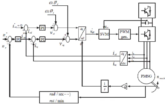
FIGURE 5.2FIELD ORIENTED CONTROL (CONSTANT TORQUE) SCHEMATIC ... 39

FIGURE 5.3FIELD ORIENTED CONTROL (CONSTANT SPEED) SCHEMATIC ... 40

FIGURE 6.1TIME RESPONSE OF THE CLOSED LOOP CURRENT CONTROLLERS. ... 48

FIGURE 6.2FREQUENCY RESPONSE OF THE CLOSED LOOP CURRENT CONTROLLERS ... 48

FIGURE 6.3REFERENCE TRACKING OF THE 𝑖𝑑 CONTROLLER ... 49

FIGURE 6.4ERROR OF THE SYSTEM ... 49

FIGURE 6.5ERROR OF THE SYSTEM CONTROLLER ... 50

FIGURE 6.6REFERENCE TRACKING OF THE I_Q CONTROLLER ... 50

FIGURE 6.7REFERENCE TRACKING I_D CURRENT ... 51

FIGURE 6.8REFERENCE TRACKING I_Q CURRENT ... 51

FIGURE 6.9DELAY IN I_Q OVER I_Q,REF ... 52

FIGURE 6.10ERROR OF I_Q ... 52

FIGURE 6.11ERROR OF I_Q FIRST CHANGE ... 53

FIGURE 6.12ERROR OF I_Q SECOND CHANGE... 53

FIGURE 6.13TIME RESPONSE OF SPEED CONTROLLER ... 54

FIGURE 6.14BODE PLOT OF SPEED CONTROLLER ... 55

FIGURE 6.15DISTURBANCE:LOAD TORQUE ... 56

FIGURE 6.16REFERENCE TRACKING OF SPEED CONTROLLER (RAMP) ... 56

FIGURE 6.17FIRST CHANGE IN SPEED BY DISTURBANCE ... 57

FIGURE 6.18SECOND CHANGE IN SPEED BY THE DISTURBANCE ... 57

FIGURE 6.19SPEED ERROR... 58

FIGURE 6.20REFERENCE TRACKING OF THE SPEED CONTROLLER (IMPULSE) ... 58

FIGURE 6.21FIRST CHANGE IN SPEED ... 59

FIGURE 6.22SECOND AND THIRD CHANGE IN SPEED ... 59

FIGURE 6.23ERROR IN SPEED CONTROLLER ... 59

FIGURE 6.24STEP RESPONSE OF DC VOLTAGE PI... 60

FIGURE 6.25BODE PLOT OF DC VOLTAGE PI ... 60

FIGURE 6.26DISTURBANCE:LOAD CURRENT ... 61

FIGURE 6.27ERROR IN DC VOLTAGE BUS ... 61

FIGURE 6.28REFERENCE TRACKING OF DC VOLTAGE ... 62

FIGURE 6.29ERROR TRACK IN DCVOLTAGE ZOOM ... 62

FIGURE 6.30DIRECT VOLTAGE ... 63

FIGURE 6.31REFERENCE TRACKING IN QUADRATURE CURRENT ... 63

FIGURE 6.32ERROR OF QUADRATURE CURRENT ... 63

FIGURE 6.33REFERENCE TRACKING IN DIRECT CURRENT AXIS ... 64

FIGURE 6.34ERROR IN DIRECT CURRENT AXIS ... 64

(13)

xi

List of Tables

TABLE 3.1ADVANTAGES AND DISADVANTAGES OF CERTAIN DYNAMOMETER ... 18

TABLE 5.1LOGIC TABLE IN TENS OF WATTS ... 44

TABLE 5.2LOGIC TABLE IN HUNDREDS OF WATTS ... 44

(14)

(15)

1

Chapter 1

1. Introduction

1.1 Motivation

The internal combustion engine is one of the best machines to introduce the student of engineering to the practical aspect of the engineer’s work. The engine is a relatively complicated machine capable of presenting many problems and faults. As A.J. Martyr [1] says “A few hours in the engine testing laboratory are perhaps one of the best possible introduction to the real world of engineering”. To test an engine are needed many fields of study. Not only mechanics, but also, electronics, computer science, chemistry, fluid dynamics, among others. Is in the interaction between many system and fields of study that relays the challenging task. Another thing that motivates the author is to provide the ground bases for future work in this matter, Not only for learning purposes but also for future researches and consequently dynamize the university and perhaps certain industries.

1.2 Main Goals

To completely describe and dimension a test cell goes beyond one person’s work. Trying to achieve it in only one dissertation means to neglect certain important parameters and systems. With that in mind this work aims, mainly, to bring together some important aspect of the tests cell components. Those components are: Firstly the engine and what are the measurement needed to identify it. Second, some review of the sensors used to measure the engine. Third describe and bring together some physical aspects of what compose a good data acquisition system. And last but not least, develop the control of one of the most important systems that composes the test cell, the dynamometer.

1.3 Task Overview

The Chapter 2: reviews the reciprocating engine, as well of all the main variables that are needed to be measured by de test stand. In chapter 3: the measuring techniques and sensors needed to obtain the data to identify and map the engine. In Chapter 4: reviews the techniques to achieve good data acquisition. Chapter 5: Describes the controllers’ principles and configurations. The Chapter 6: the simulations results are listed. And last, the Chapter 7: The Conclusions of this work are listed.

(16)

(17)

3

Chapter 2

2. The internal combustion Engine

The purpose of the Internal Combustion (IC) engines is to transform chemical energy, contained within fuel, to mechanical power. In the IC engines the chemical energy is released by oxidizing the fuel inside the engine. The working fluids are the air-fuel mixture before combustion and the burned product after that. The work transfer occurs between the admission of the air-fuel mixture in the combustion chamber and the exhaust, where the burned gasses are released from the system.

There are a wide variety of IC engines. The most know ones are the gas turbine or jet engine, the rocket engine, and the reciprocating engine. For the purpose of this work only the last one will be explained, the reciprocating engine.

The reciprocating engines are the ones where the combustion it’s enclosed within a cylinder and a piston moves back and forth inside the cylinder, transmitting the power generated to the drive shaft through a connecting rod and a crank mechanism.

To facilitate the understanding, from now on, the reciprocating engine will be called as IC engine.

2.2 Engine classifications

The IC engines can be classified by the groups below[2]:

 Application. Automobile, light aircraft, marine, power generation, etc.

 Basic engine design. Reciprocating or piston engines, also subdivided for the arrangement of the cylinders: in-line, V, opposed, radial, etc. Rotary engines: Wankel and different geometries.

 Working cycle. Four-stroke cycle: turbo-charged, supercharged or naturally aspirated. Two-stroke cycle: crankcase scavenged, and also as the four-strokes turbo and supercharged.

 Fuel. Petrol or gasoline, fuel oil or diesel, natural gas, LPG (liquid petroleum gas), hydrogen, methanol and ethanol, or the combination of some listed before.

 Valve design location. Loop-scavenged porting, the exhaust and inlet ports or valves are on the same side, at one end, of the cylinder. Cross-scavenged, the exhaust and inlet valves or ports are on the opposite sides, at one end, of the cylinder.

(18)

Uniflow-4

scavenged, inlet and exhaust ports or valves are at different ends of a cylinder. Overhead valves or I-head. Under head valves or L-head. Rotary, etc.

 Method of mixture preparation. Carburation. Direct injection into the cylinder. Fuel injection into intake manifold.

 Method of ignition. Spark-ignition and stratified charges (the first is used when the mixture is uniform, and the last is used when is non-uniform). Compression ignition.  Combustion chamber design. Open chamber: blow-in-piston, hemisphere, disc, and

others. Divided chambers: swirl chamber and pre-chambers, etc.

 Method of cooling. Air cooled, water cooled, uncooled or cooled by natural convection and radiation.

 Method of load control. Throttling of air and fuel together. Control of fuel alone. Or a combination of both.

2.3 Engine operating cycle

As described previously, when the cylinder moves, generates a rotation of the crankshaft within it axis. There are two times where the piston comes at rest: the top-centre, TC, located at 0º of the shaft rotation, and bottom-centre, BC, located at 180º of the shaft rotation. Those two instances defines the minimum and maximum volumes inside the cylinder. When the piston it’s at TC the volume inside its minimum and it’s called clearance volume (𝑉𝑐), when the piston is at BC the volume is at its maximum and it’s called total volume (𝑉𝑡). The difference between those volumes mentioned before it’s called swept or displacement (𝑉𝑑), and the ratio of the maximum to minimum volume is called compression ratio (𝑟𝑐).

The two greatest types of IC engines are the four-strokes and the two-strokes. Of which the first is more common used.

The four-stroke engine cycle consists in four strokes of the piston to complete the cycle in which are two revolutions of the shaft. In this cycle has what it called a power stroke and it’s used in both compression-ignition and spark ignition.

(19)

5 Figure 2.1 Cylinder and shaft representation [2]

The stroke of an engine are:

1. The admission or intake stroke. Which draw the air-fuel mixture into the cylinder. It begins when the piston it’s at TC and ends when the piston it’s at BC. The intake valve opens before the stroke it’s initiated and close a few moments after it end.

2. The compression stroke. When the piston reach BC and after both valves are closed it begins to compress the volume inside the cylinder which rapidly increase the pressure in it. Shortly before the end of this stroke or near TC the combustion begins.

3. The expansion stroke. As the combustion begins it increase the temperature and pressure forcing the piston to go from TC to BC which relates in a shaft rotation, and the work done by this stroke it’s approximately five times greater than what is needed in the compression stroke. Closely to BC the exhaust valve opens and decrease pressure to closely the exhaust pressure (blowdown).

(20)

6

4. The exhaust stroke. In this stroke, and as the piston moves, the remaining gases contained inside the cylinder are released from the system. When the piston is near TC the inlet valve opens: first to equalise the remaining pressure to near the exhaust as sometime the combustion pressure it’s considerably high than the exhaust and the fluid could not exit the chamber in time, and second to give place to a new cycle that begins just after the exhaust valve closes.

Figure 2.2 Four stokes engine cycle [2]

2.4 Important Engine Characteristics

To characterize the performance of an engine some basic parameters and geometrical relationships are commonly used [2]:

1. The maximum power (or the maximum torque) available at each speed within the useful

engine operating range

2. The range of speed and power over which engine operation is satisfactory The following

performance definitions are commonly used:

a) Maximum rated power. The highest power an engine is allowed to develop for short periods of operation.

b) Normal rated power. The highest power an engine is allowed to develop in continuous operation.

(21)

7

2.5 Properties of the Reciprocating Engine

There are many parameters that defines the reciprocating engine and its properties some of those, the most important, are listed below.

Figure 2.3 Geometry of cylinder, piston, connecting rod, and crankshaft where 𝐵 = bore, 𝐿 = stroke, 𝑙 = connecting road length, a = crank radius, 𝜃 = crank angle [2]

 Compression ratio 𝑟𝑐: 𝑟𝑐 = 𝑚𝑎𝑥𝑖𝑚𝑢𝑚 𝑐𝑦𝑙𝑖𝑛𝑑𝑒𝑟 𝑣𝑜𝑙𝑢𝑚𝑒 𝑚𝑖𝑛𝑖𝑚𝑢𝑚 𝑐𝑦𝑙𝑖𝑛𝑑𝑒𝑟 𝑣𝑜𝑙𝑢𝑚𝑒 = 𝑉𝑑+ 𝑉𝑐 𝑉𝑐 (2.1)

 Ratio of cylinder bore to piston stroke: 𝑅𝑏𝑠=

𝐵 𝐿

(2.2)  Ratio of connecting rod length to crank radius:

𝑅 = 𝑙

𝑎 (2.3)

 In addition, the stroke and crank radius are related by:

(22)

8

 The cylinder volume at any crank position is given by:

𝑉 = 𝑉𝑐+ 𝜋𝐵2

4 (𝑙 + 𝑎 − 𝑠)

(2.5)

o Where, 𝑠 is the distance between the crank axis and piston axis and is given by:

𝑠 = 𝑎 cos 𝜃 + √𝑙2_{+ 𝑎}2_{− 𝑠𝑖𝑛}2_𝜃

(2.6)

 The angle 𝜃, defined as shown in Fig. 2-1, is called the crank angle. Equation (2.4) with the above definitions can be rearranged:

𝑉 𝑉𝑐 = 1 +1 2(𝑟𝑐− 1) (𝑅 + 1 − cos 𝜃 × √𝑅 2_{− 𝑠𝑖𝑛}2_𝜃) (2.7)

 The combustion chamber surface area A at any crank position is given by

𝐴 = 𝐴𝑐ℎ+ 𝐴𝑝+ π B (l + a − s)

(2.8)

o Where,𝐴𝑐ℎis the cylinder head surface area and 𝐴𝑝 is the piston crown area.

 For a flat-topped piston 𝐴𝑝= 𝜋𝐵2

4

o Using (2.7) , (2.8) can be rearranged.

𝐴 = 𝐴𝑐ℎ+ 𝐴𝑝+π B

2 (𝑅 + 1 − cos 𝜃 × √𝑅

(23)

9  Another important characteristic is the mean piston speed 𝑆̅̅̅ 𝑝

𝑆𝑝

̅̅̅ = 2 𝐿 𝑁 _(2.10)

o Where 𝑁 is the rotational speed of the crank shaft

 Often a more important parameter is the instantaneous piston speed and its given by :

𝑆𝑝= 𝑑𝑠 𝑑𝑡

(2.11)

 The ratio between the two equations above is given by 𝑆𝑝 𝑆𝑝 ̅̅̅= π 2 sin 𝜃 (1 + cos 𝜃 √𝑅2_{− 𝑠𝑖𝑛}2_𝜃) (2.12)

2.5.1 Torque and Power

The torque output of an engine an important measurement to evaluate an engine’s ability to do work. Since the torque is a moment that mean that is the product of a force and a length [2]. The torque equation can be written as:

𝑇 = 𝐹 × 𝑏 (2.13)

Where, F is the force applied by the arm and b is the arm length

The power P delivered by the engine, which is the rate at which work is done, is the product of torque and angular speed:

𝑃 = 2𝜋𝑁𝑇 (2.14)

2.5.2 Mean Effective Pressure

Mean effective pressure (mep) is a more useful parameter to evaluate the engine performance and is obtained by dividing the work per cycle by the cylinder displaced volume per cylinder. This parameter has units of force per unit area.

The work per cycle is given by:

𝑊𝑜𝑟𝑘 𝑝𝑒𝑟 𝑐𝑦𝑐𝑙𝑒 =𝑃 𝑛𝑟 𝑁

(24)

10

Where 𝑛𝑟, is the number of crank revolutions for each power stroke per cylinder (two for four-stroke cycles; one for two-four-stroke cycles), then

𝑚𝑒𝑝 =𝑃 𝑛𝑅 𝑁𝑉𝑑

(2.16)

2.5.3 Specific Fuel Consumption and efficiency

The specific fuel consumption (sfc) is the fuel flow rate per unit power output. It measures how efficiently an engine is using the fuel supplied to produce work:

𝑠𝑓𝑐 =𝑚̇𝑓 𝑃

(2.17)

2.5.4 Fuel Conversion Efficiency

Since the sfc has units, a dimensionless parameter would have more value. This can be achieved by relating the engine output (power or work per cycle) to the fuel flow.

The fuel energy supplied which can be released by combustion is given by the mass of fuel supplied to the engine per cycle times the heating value of the fuel.

The heating value of a fuel,𝑄𝐻𝑉, defines its energy content. It is determined in a standardized test procedure in which a known mass of fuel is fully burned with air, and the thermal energy released by the combustion process is absorbed by a calorimeter as the combustion products cool down to their original temperature. This measure of an engine's "efficiency," is given by:

𝜂𝑉= 𝑊𝑐 𝑚𝑓 𝑄𝐻𝑉 = (𝑃𝑛𝑅/𝑁) (𝑚̇ 𝑛𝑓 𝑅/𝑁)𝑄𝐻𝑉 = 𝑃 𝑚𝑓̇ 𝑄𝐻𝑉 (2.18)

Where 𝑚𝑓 is the mass of fuel inducted per cycle.

𝜂𝑉= 1 𝑠𝑓𝑐𝑄𝐻𝑉

(2.19)

2.5.5 Air/Fuel ratio and Fuel/Air ratio

The ratio of the air mass flow rate 𝑚̇ and the fuel mass flow rate 𝑚𝑎 ̇ is useful to define an 𝑓 engine operating conditions. It can be expressed in two ways:

(25)

11 Air/Fuel ratio (𝐴 𝐹⁄ ) =𝑚𝑎̇ 𝑚𝑓̇ (2.20) Fuel/Air ratio (𝐹 𝐴⁄ ) =𝑚𝑓̇ 𝑚̇𝑎 (2.21)

2.5.5 Volumetric Efficiency

The volumetric efficiency is a parameter used to measure the effectiveness of an engine’s induction process. From the moment the air is in the system, there are many stages in it that restrict the amount of air of which displacement can induct. This parameter can be expressed as:

𝜂𝑉= 2 𝑚̇ 𝑎 𝜌𝑎,𝑖𝑉𝑑𝑁

(2.22)

Where 𝜌𝑎,𝑖is the inlet air density, alternately the volumetric efficiency can be expressed [2]:

𝜂𝑉= 2 𝑚𝑎 𝜌𝑎,𝑖𝑉𝑑

(2.23)

Where 𝑚𝑎 is the mass of air inducted into the cylinder per cycle. The inlet density may either be taken as atmosphere air density (in which case 𝜂𝑉, measures the pumping performance of the entire inlet system) or may be taken as the air density in the inlet manifold (in which case 𝜂𝑉, measures the pumping performance of the inlet port and valve only).

2.5.6 Engine Specific Weight and Specific Volume

The two parameters, specific weight and specific volume, are a useful way comparing those attributes from one engine to another.

𝑆𝑝𝑒𝑐𝑖𝑓𝑖𝑐 𝑤𝑒𝑖𝑔ℎ𝑡 = engine weight 𝑟𝑎𝑡𝑒𝑑 𝑝𝑜𝑤𝑒𝑟 (2.24) 𝑆𝑝𝑒𝑐𝑖𝑓𝑖𝑐 𝑣𝑜𝑙𝑢𝑚𝑒 = 𝑒𝑛𝑔𝑖𝑛𝑒 𝑣𝑜𝑙𝑢𝑚𝑒 𝑟𝑎𝑡𝑒𝑑 𝑝𝑜𝑤𝑒𝑟 (2.25)

(26)

12

2.6 Relationship between performance parameters

The importance of all the parameters defined above becomes evident when power, torque, and mean effective pressure are expressed in terms of these parameters.

Combining the three parameters mentioned earlier, and combining with the fuel conversion efficiency, fuel-air ratio, the following relationships between engine performance parameters can be developed [2]. For power P:

𝑃 =𝜂𝑓𝑚𝑎 𝑁 𝑄𝐻𝑉(𝐹 𝐴⁄ ) 𝜂𝑟

(2.26)

For four-stroke cycle engines, volumetric efficiency can be introduced:

𝑃 =𝜂𝑓 𝜂𝑉 𝑁 𝑄𝐻𝑉 𝜌𝑎,𝑖 (𝐹 𝐴⁄ ) 2 (2.27) For torque T 𝑇 =𝜂𝑓 𝜂𝑉 𝑄𝐻𝑉 𝜌𝑎,𝑖 (𝐹 𝐴⁄ ) 4𝜋 (2.28)

The mean effective pressure can be written as:

𝑚𝑒𝑝 = 𝜂𝑓 𝜂𝑉 𝑄𝐻𝑉 𝜌𝑎,𝑖 (𝐹 𝐴)⁄ (2.29) The power per unit piston area, often called the specific power, is a measure of the available piston area regardless of cylinder size. The specific power can be expressed as:

 For power P: 𝑃 𝐴𝑝 =𝜂𝑓 𝜂𝑉 𝑁 𝐿 𝑄𝐻𝑉 𝜌𝑎,𝑖 (𝐹 𝐴⁄ ) 2 (2.30)

 Mean piston speed can be introduced, to give 𝑃

𝐴𝑝

=𝜂𝑓 𝜂𝑉 𝑆̅̅̅ 𝑄𝑝 𝐻𝑉 𝜌𝑎,𝑖 (𝐹 𝐴)⁄ 4

(2.31)

Specific power is thus proportional to the product of mean effective pressure and mean piston speed. These relationships illustrate the direct importance to engine performance of:

(27)

13 1. High fuel conversion efficiency

2. High volumetric efficiency

3. Increasing the output of a given displacement engine by increasing the inlet air density 4. Maximum fuel-air ratio that can be usefully burned in the engine

5. High mean piston speed

2.7 Engine Performance Data

Engine ratings usually indicate the highest power at which manufacturers expect their products to give satisfactory economy, reliability, and durability under service conditions. Maximum torque, and the speed at which it is achieved, is usually given also. The most significant measures, at the operating point indicated are[2]:

 Mean piston speed. Measures comparative success in handling loads due to inertia of the parts, resistance to air flow, and/oi engine friction.

 Brake mean effective pressure. In naturally aspirated engines bmep is not stress limited. It then reflects the product of volumetric efficiency (ability to induct air), fuel-air ratio (effectiveness of fuel-air utilization in combustion), and fuel conversion efficiency. In supercharged engines bmep indicates the degree of success in handling higher gas pressures and thermal loading.

 Power per unit piston area. Measures the effectiveness with which the piston area is used, regardless of cylinder size.

 Specific weight. Indicates relative economy with which materials are used.

 Specific volume. Indicates relative effectiveness with which engine space has been utilized. At all speeds at which the engine will be used with full throttle or with maximum fuel-pump setting:

 Brake mean effective pressure. Measures ability to obtain/provide high air flow and use it effectively over the full range.

 At all useful regimes of operation and particularly in those regimes where the engine is run for long periods of time:

(28)

(29)

15

Chapter 3 3. The Test Cell

The purpose of this chapter is to introduce the principal systems and fundamentally describe the measurement needed to characterize a reciprocating engine. The test stand is a mix of complex machinery and instrumentation, normally housed in a building designed for its purpose. The main objective of the system is to merge all that machinery and instrumentation into as is commonly said ‘well-oiled machine’. The common product of the test stand systems is data, that later, will be used to homologate, identify, develop or modify performance criteria of the parts which compose the engine. In this chapter can be found the principal measurements, as well a set of transducers (sensors or actuators) needed to obtain the referred data.

Figure 3.1.1 Engine test cell example [1]

3.2 The dynamometer

As it was said earlier in this work the primary function of the dynamometer is to resist the load of the prime mover, in this case the reciprocating engine. The dynamometer also, measures the torque and speed of the prime mover in order to calculate the power. The power obtained in the dynamometer is called brake power, as it name says the dynamometer acts as a “brake” to the engine.

In this section the principles of torque measurement are reviewed as well as the types of dynamometers in order to give substantial knowledge in choosing the appropriate machine.

(30)

16

3.2.1 Dynamometer types

1. Hydrokinetic dynamometers (water brakes). A shaft is attached to a cylindrical rotor which turns inside a watertight casing. They work on the principle of transfer momentum from the rotor to the stator developing torque opposite to the shaft. A forced vortex is generated as consequence of this motion, leading to a high rate of turbulence in the water and the dissipation of power is in the form of heat.

There are two kinds of machines, they varies on the way in which the resisting torque is controlled[1].

a. Constant fill machines: the torque is controlled by inserting or withdrawing pairs of thin plates between rotor and stator, thus varying the extent of the development vortices.

b. Variable fill machines. In these machines, the torque absorbed is varied by adjusting the flow of water within the casing.

2. Hydrostatic dynamometers. These machines consist on combination of a fixed stroke and a positive displacement variable stroke hydraulic pump/motor, similar to that found in large off-road vehicle transmissions. The fixed stroke machine forms the dynamometer. The advantage of this non-electrical dynamometer is that can power the engine under test if it is needed.

 Electrical motor-based dynamometers. These machines transform the power absorbed into electrical energy, which is, then, transmitted to a load circuit. The energy losses within both the motor and its drive are in the form of heat and is transferred to a cooling medium, which may be water or as is more common, forced air flow.



o Direct current (d.c.) dynamometers. These machines consist essentially of a d.c. motor generator. They are robust, easily controlled, and capable of motoring and starting as well. Some disadvantages are limited maximum speed and high inertia, which can present problems of torsional vibration and limited speed changes.

o Asynchronous or induction dynamometers. They consist essentially of an induction motor with squirrel cage rotor, which is controlled by varying the supply frequency. They have a lower rotational inertia than d.c. machines of the same power and, therefore, capable of better transient performance. They have proved very robust in service requiring low maintenance.

(31)

17 o Synchronous machine, permanent magnet (PMSM) dynamometers. The units represent the latest generation of dynamometer development and while using the same drive technology as the induction dynamometers they are capable of higher dynamic performance due to the lower rotational inertia. It is this generation of machine that will provide the high dynamic test tools required by engine and vehicle system simulation in the test cell.

o Eddy-current dynamometers. These machines make use of the principle of electromagnetic induction to rise the eddy current and in turn develop torque and dissipate power. A toothed rotor of permeable steel rotates, with a fine clearance, between cooled steel loss plates. A magnetic field is induced by two annular coils located in the loss plate. This, in turn, give rise to the eddy current and dissipates power in the form of heat. The cooling system consist either in water system attached to the loss plate or a forced flux of air into the machine. The power is controlled by varying the current in the coils. On one hand, they are robust and capable of developing substantial braking torque at relatively low speeds. On the other hand they are unable to produce motoring torque.

 Friction dynamometers. These machines, consist essentially of water-cooled, single or multidisc friction brakes. They are useful for low-speed applications, and have the advantage of developing full torque down to zero speed.

3.2.2 Matching engine and dynamometer characteristics

The different types of dynamometer have significantly different properties, and this can affect the usefulness in an application. It is essential to superimpose the maximum torque– and power– speed curves on to the dynamometer envelope. The different elements of the performance envelope are as follows[1]:

 Performance limited by maximum permitted shaft torque.  Performance limited by maximum permitted power.  Maximum permitted speed.

 Minimum torque corresponding to minimum permitted.

For best accuracy, it is desirable that the dynamometer will be the smallest machine that can coup to the engine to be tested. All within the range above described.

(32)

18

3.2.3 Dynamometer comparison.

In the Table 3.1 the previously described dynamometers are listed with its advantages and disadvantages.

Table 3.1 Advantages and disadvantages of certain dynamometer

Type Advantages Disadvantages

Hydrokinetic Constant fill Cheap and robust Slow response. Difficult to

automate.

Hydrokinetic Variable fill Automated, can tolerate some amount of overload.

Can suffer of corrosion and cavitation

Hydrostatic Provides four quadrant

performance

Expensive, mechanically compressed and deal with high pressure oil

DC machine Capable of four quadrant. Well

known technology.

High inertia and high maintenance

Induction machine Low inertia and four quadrant

performance.

Expensive, fairly complex electronics

Permanent magnet

synchronous machine

Low inertia, small size and four quadrant performance

Expensive, fairly complex electronics

Eddie current Mechanically simple, low

inertia, simple control

Vulnerable to overheating and not suitable for rapid power changes

Friction High torque at low speed Limited speed range

3.3 The four quadrant of Power

The power as previously shown is the product of torque and speed. It can be measured, essentially, in four combinations: with positive speed and positive torque (quadrant I), with negative speed and positive torque (quadrant II), with negative speed and negative torque (quadrant III), and with positive speed and negative torque (quadrant IV). Since the speed is rotational, conventionally, the clock wise direction is considered positive. The torque, on the other hand, is consider positive when the dynamometer is absorbing or, in the electric machine,

(33)

19 generating and when negative is motoring. When measuring the power the only it magnitude is taken in to account. Consequently the signal of the power depends on the torque.

Figure 3.2 Speed-Torque map[1]

3.3.1 Measurement of torque

There are many approaches to measure torque, for example, in electric machines it can be achieved by measuring the electric power of the output or input (depending on the machine). The two most common methods to obtain torque measurements are[1]:

 In-line shafts or torque flanges. This method consist in mounting the torque sensor in the drive line between the prime mover and the brake machine. There are different kinds of sensor, each with its own method of sensing. One of the disadvantages of this method is the necessity of applying torque corrections under transient conditions.  Trunnion-mounted or cradle machines. In this method the power absorbing element

of the machine is mounted coaxially with the machine shaft and, normally is mounted on bearings. The torque is measured, and restrained by a transducer sensing tangentially, and at known radius of the machine’s axis. In traditional machines the measurement of torque was achieved by balancing dead weights and a spring against the torque absorber. The most modern uses a force transducer, commonly the load cell.

The last method will give more accurate torque readings, for steady state, than the first. Some of the advantages are listed below:

 The in-line torque sensor loses resolution as it has to be oversized to prevent eventual failure with a torque peak.

(34)

20

 As the sensor is part of the drive line it requires very careful installation to avoid imposition of axial stresses.

 Is difficult to protect from temperature fluctuations within and around the drive-line.  It is not possible to verify the measured torque of an in-line device during operation.

3.3.2 Measurement of angular speed

There are many methods to measure angular speed. Mostly are either electro-mechanical or electro-magnetic. The angular speed can be measured in the engine’s shaft or in the dynamometer. However, when using transmission or belts is extremely recommended to measure both to confirm the ratios and/or estimate losses. The main types of speed sensors or tachometers are:

Impulse Tachometers

In this device, a small spindle is used to make physical contact with the rotating shaft so that will rotate at the same velocity. At the same time the spindle is attached to a reverse switch which reverse twice in each revolution of the shaft. The reversing switch creates a link between the charging potential to a capacitor in each direction, and with each pulse, a signal is given to the measurement device (ADC or ammeter)[3].

Rotary Encoders

In the rotary encoder, the shaft turns a disk which has a radial pattern with a unique code for distinct position. On the back of the disk are light emitting diodes, allowing a photo-transistor to read the pattern. Normally, the encoder is made by two sets of discs both with the same pattern but at different positions. By comparing the readings of the two the direction of rotation ca be known. The resolution of the encoder depends on the pattern which is binary so the resolution will be2𝑛_[3]

Photoelectric Sensors

In the photoelectric sensor a light beam is modulated by the rotating member, which consist on a reflective material attached to the object or shaft, and then sensed by a photocell. In this method the speed estimation is proportional to the frequency of the pulse sensed in the photocell. Another method with this device, if the object is perforated, consist in locate a light emitter and the photocell in the opposite sides of the object [3].

AC Tachometers

The AC tachometer is an electromechanical device very similar to an induction motor. It is made of a primary winding attached to the rotor and a secondary winding placed 90 degrees to the primary. When the rotor begins to turn, a sinusoidal voltage is induced into the secondary winding which is proportional to the rotor speed [3].

(35)

21

DC Tachometer

The DC tachometer, is made by a winding located on the shaft and a permanent magnet. As the speed increases, a sinusoidal voltage is induced by the relative difference in speeds between the magnets and the winding, which then is converted into a d.c. voltage through the commutator, in the same way as the generator[3].

Reed Switch

The reed switch consist of a multipole magnet attached to the rotor and a stationary magnetic reed switch attached near to the magnet. As the magnets passes onto the switch, the polarity of the magnets causes the switch to open and close a circuit. The frequency of the pulse is proportional to the rotational speed of the shaft.

Hall-Effect Sensor

A current is passed through a semiconductor material. When a magnetic field is applied perpendicularly to the surface of this material, a voltage is induced. This voltage is called Hall voltage and is proportional to the applied field intensity.

Magneto-resistive Sensors

In magneto-resistive sensors, the resistance of the sensing element varies with the direction and proximity of a magnetic field. In these sensors, a small voltage is induced when a magnetic surface passes in near proximity to the sensing element[3].

3.4 Air Flow Measurement

The primary working fluid of an engine is the air. Which mean that the air flow is one of the most important measurements in an engine. The fuel function is to provide the system with heat. The accurate measurement of the air consumption of an internal combustion engine is a matter of some complexity but of great importance.

The air can be affected by many factors and accurately measure its flow can be difficult. In the automotive industry is usually corrected as a function of four parameters: temperature, pressure, moisture content or humidity and the impurities.

The influence, on the air flow, of the parameters previously mentioned are:

 Atmospheric Pressure: the pressure affects directly the mass of air admitted, as it varies the density of the air, which is directly proportional to the absolute pressure.  Air temperature: the variation in temperature have an effect of the same order of

magnitude as the pressure variation. As the temperature, also, affect the density but is inversely proportional to it.

(36)

22

 The moist content: the effect of this one, when compared to the other two, is relatively small. The moist is a combination of air and water vapour, because of that the oxygen for combustion contained in the air is higher in the absence of water vapour. It is to be noted that the effect of temperature in the moist can affect largely the magnitude of it.

The air box method

The simplest method to achieve this measurement is the air box, which measure the pressure drop across a box. Normally, it is measured by a sharp edge orifice on the side of the box, coupled to the inlet of the engine. The box has to have sufficient volume to damp flux pulsations into the engine. One of the disadvantages of this method is that the for pressure difference varies with the square of the flow rate and that implies insufficient precision at low rate. A common practice in this type of method is to vary the size of the orifice according to the flow expected.

Positive displacement flow meters

In this method the air flow is measured as a function of the rotational speed of two rotating shafts contained within a certain volume. The majority of the positive displacement flow meter operates on the principle of Root blower. Some disadvantages are the cost and it sensitivity to contamination in the flow. The main advantages are the accuracy and simplicity[3].

Hot wire or hot film anemometer devices

This method is based on the principle of the cooling effect of a gas flow in a heated film or wire surface. The heat loss is directly proportional to the air mass flow rate and has a good tolerance for air contamination. The disadvantages is that has a difficult calibration and for that the calibration must be made by the manufacturer[3].

Lucas–Dawe air mass flow meter

In this method the air is ionized within the tube, the ionized air flows in the direction of the tube. The air flow deflects the ion current. And, as consequence of that, the difference in current is a function of the flow.

The viscous flow air meter

The viscous flow meter is almost the same as the air box meter with the difference that the orifice is substituted by a plate with small orifices, usually in triangular form. As consequence of the small orifices, air flow will be relatively laminar which mean that the pressure drop across the element could be approximately directly proportional to the velocity of the flow[3].

(37)

23 One of the advantages is that the average pressure drop permit calculation of the flow rate. The disadvantage is that the device needs to be calibrated against a standard device.

3.5. Temperature Measurements

Thermistor

The thermistor, as it name says, is a thermal resistor i.e. a resistor that change it resistance with temperature. All the resistors exhibit this property, but the thermistor is conceived in a way that it resistance change drastically with the small change of temperature. Normally the change in resistance are around 100 ohm or more per degree of temperature.

There are two types of thermistors, the NTC (Negative Temperature Coefficient) and the PTC (Positive Temperature Coefficient). That mean that, the first, decrease it resistance with the increase of temperature, and the second, increase it resistance with increase of temperature.

Thermocouple

The thermocouple exploit the Seebeck effect to read a temperature difference. The Seebeck effect is the amount of electric potential (voltage) present in a circuit made by two different metals with, at least two, junctions at different temperatures. This, temperature-induced, electrical potential is called an electromotive force and abbreviated as EMF.

To obtain a proper measure of the thermocouple i.e. to ensure the EMF change in proportion to the temperature. One junction must be held at constant temperature. In theory a thermocouple could be made by any two dissimilar metals. In practice, mainly because of their temperature coefficient are highly repeatable and outputs at relatively large voltage, only few combinations have become standard.The most common thermocouple types are called J, K, T, and E, followed by N28, N14, S, R, and B.

Resistance Temperature Detector (RTD)

The Resistance Temperature Detector (RTD), uses the same principals as the thermistor. The two are composed of materials with known resistance vs temperature (see thermistor). Unlike the thermistor, which is generally made of a semiconductor material, the RTD is made of a metal with high positive temperature coefficient of resistance. There are mainly two types of RTDs:

 The Wire-wound: It consist on a wire, with small diameter, wired into a coil. This configuration it is needed to be isolated to protect them from shock and vibrations. It is achieved by using a combination of ceramic bobbin with glass or epoxy over the coil and welded connections.

(38)

24

 The Thin-film element: It consist on a very thin layer of the base metal, deposited onto a ceramic substrate, and then laser trimmed. This kind of approach is more cost effective since the same resistance is achieved with less base metal.

Integrated Circuit Temperature Sensor (ICTS)

ICTS also referred as Monolithic sensor depends on the property of some material which is temperature dependent. This property is preferably to be a linear function in the range that is pretend to be used (temperature range). One example of that is the base emitter voltasge 𝑉𝐵𝐸 of a silicon NPN transistor, who has such temperature dependence in a set certain range of temperature.This value of 𝑉𝐵𝐸 varies of varies over a production range and the calibration errors are not specified nor ensured in production. Furthermore, there’s a drift in the linearity of the sensor that can achieve as 3ºC or 4ºC over a full range of temperature. A more exact approach has been developed that relays in the difference in the base-emitter voltage of two transistors operated at different current densities.

3.6 Pressure transducers

The Load Transducer

The strain gauge: The most usual form of strain measurement uses a resistive strain gauge. This kind of strain gauge, commonly, consist in a thin wire which is attached firmly to the material in which strain is to be detected. Then it will be connected as part of a resistance circuit. The strain gauge is an example of the piezoresistive principle, because of the change of resistance is due to the deformation of the crystal structure in the material that is used for sensing. The load cell: The load cell could be defined as a series of strain gauges, usually four, connected on a Wheatstone-bridge circuit. That mean that there will be two parallel circuit with two strain gauges connected in series, each. The load cell as a whole is a passive transducer, which means that it is need to be excited in order to obtain any measurement.

Optical Transducer

The optical pressure sensor consist on a diaphragm that is excited by the elastic pressure applied on it, which in turn lift a vane in front of a light beam (infrared). The light that passes the vane is measured by a photo-sensitive diode. This sensor is insensitive to temperature variations and the repeatability and hysteresis errors are negligible.

Potentiometric Transducer

This transducer a change in pressure provoke movement in a precision potentiometer linked by a rod. The contacting rod is usually made of noble material. These transducer requires the least

(39)

25 signal conditioning and therefore are the least expensive. Their disadvantages are the low life expectancy and high noise levels.

(40)

(41)

27

Chapter 4

4. Data Acquisition System

4.2 Signal

A signal could be any type of physical quantity that varies in relation to an independent variable, like time or space. Within the data acquisition system, often the signal is referred to an electrical signal that varies in electric potential, current or magnetic property in relation to time, frequency or amplitude. The electrical signals, then, are classified in two categories, the analogue and digital. The analogue signal is a continuous signal normally represented as a sinusoidal wave, and can vary in amplitude or in frequency Figure. On the contrary the digital signal is a discrete signal, which mean only can assume a finite number of states. It have a constant frequency and only change in amplitude. The digital signal, in signal processing, is binary that means, it can only assume two states, high or low. Each of those signal has its own properties and importance which mean that they need to be handled differently. The type of processing it will be discussed later on in this chapter.

4.3 Transducer

The transducer is an instrument that can transform one form of energy to another. For a data acquisition system the transducer is used in a way that can transform a physical effect (like temperature, pressure or flow) to an electrical signal or vice versa. When the process occurs in a way that a physical signal is needed to transform into an electrical signal, the transducer is called sensor. As it sense the phenomena and transform it in a way that can be interpreted. When occurs in the other way, it is called an actuator. As given an input, is given, often electrical, it transform in a way that can “actuate” or change the state of the system[3].

4.4 Signal conditioning

Since every sensor and actuator work with its own properties, some kind of signal manipulation is needed to normalize and properly control the process (properly read in the case of the sensor). This action is called signal condition, as it condition the signal between the transducer and the control block. For sensors, normally between them and the analogic to digital converter

(42)

28

(ADC) and for the transducer from de digital to analogic converter (DAC) or the pulse-width modulation (PWM) to them. The most common signal conditioning processes are the following:

4.4.1 Amplification

The amplification process aims to increase the voltage level, for example to maximize the resolution and sensitivity of an ADC. There is a wide variety of methods to achieve that. Some of those methods are:

 The operational amplifier is one circuit, often portrayed as a simple logical function block with external resistors and capacitors to determine the gain of the system. Most of the operational amplifiers are distributed in two groups, the inverting amplifier and the non-inverting. However there are some special cases in those two groups like unity-gain amplifiers, the follower and the difference amplifiers. The main groups are described as following:

o Inverting Amplifier Stages this type of amplifier accepts an input signal, amplifies it, and invert the polarity. The gain of the input voltage is controlled by a voltage divider.

o Non-Inverting Amplifier this type of amplifier is similar to inverting type but the phase of the output signal matches the input. Also, the output gain depends on the voltage divider

 The programmable gain amplifier is typically a non-inverting amplifier but it gain is digitally controlled by a bank of resistors connected in a feedback loop. A controller sense the input amplitude and, then, send a signal to a switch to properly adjust the gain in the voltage divider. The input signal can then be measure without distortion.

4.4.2 Attenuation

The attenuation process is the opposite of the amplification. It decrease the signal amplitude. Is commonly used when the voltage or current are beyond the range of some circuit or ADC. The single most common technique is the voltage divider, which consist in a set of resistances connected in series. The voltage drop in the first resistance will give the desired range. Sometimes the impedance of the voltage divider is too large to be sensed by an instrument. To reduce that is commonly used a unity-gain amplifier.

4.4.3 Filtering

Filtering is used to stabilize a signal and rejects unwanted noise within a certain range of frequencies. The filtering can produce a clear signal and there are two ways to achieve that: as analogue filtering or digital filtering, which is normally achieved with the help of

(43)

micro-29 processors. Regardless of the signal to process, the filters have three main topologies. They are[4]:

 Low-Pass Filter The low-pass filter rejects the higher frequencies depending on the magnitude of the high frequency and the cornering frequency. This topology is widely use to clear high frequency noise form a transducer, which normally is affected by electromagnetic noise coming from the surroundings. The best way to apply the low-pass filter, when using sensors that need amplification, is to install it prior to the amplification. In that way the signal coming from the amplifier has not amplified the noise.

 High-Pass Filters The high-pass filter rejects the low-frequencies. They attenuate lower frequencies that are not desired. It is commonly used when analysing vibrations, for example from a machine. This measurement can be corrupted by low frequencies, interference from a certain vibration within a power transformer’s core.



Band-pass filter: Is a combination of the two topologies above. Ideally, it reject all but

a certain range of frequencies. They are commonly used in wireless emitters and receivers and in ultrasound sensors.

4.4.4 Isolation

As it name says the isolation is use to isolate a system or sub-system from a signal that are outside the power range of it. Is normally used in conjunction with attenuation to protect, for example, to dangerous voltages. Another common use for isolation is to protect certain transducer from external noises.

4.4.5 Excitation

Excitation is the procedure to add current to a device. This type of signal conditioning is used in transducers that need external source to work. For example accelerometers, strain gauges and thermistors.

4.5 Analogue-to-Digital Converter

The Analogue-to-digital converter is a module or system that transform an analogue input signal, compared to a reference one (voltage or current), into a digital signal output. The input range is determined by the reference voltage (𝑣𝑟𝑒𝑓) applied to the ADC. [5]This reference voltage can be internal or external. If the input voltage (𝑣𝑖𝑛) is greater than the reference one it will saturate, so it need to be guaranteed that the input signal does not exceed the reference.

(44)

30

Then the entire input range is divided into small ranges. Each of this ranges or sub-ranges has assigned a digital output code. The total number of subranges is called resolution and, usually, is given in power of two,2𝑛_{(where n is the number of subranges or bits).}

The ideal ADC has infinite resolution, which mean that every possible analogue signal value has a unique digital output code within a certain conversion range. In a real ADC, due to the nature of the digital signal, there is always a gap between one digital number and the consecutive one. The value of the “gap” depends on the minimum value the ADC can resolve and is called quantization. In other words, the quantization is the range of the least significant bit (LSB) can achieve, and can be mathematically described as[5]:

𝑄𝑢𝑎𝑛𝑡𝑖𝑧𝑎𝑡𝑖𝑜𝑛 = 𝐴𝐷𝐶 𝑟𝑎𝑛𝑔𝑒 𝐴𝐷𝐶 𝑟𝑒𝑠𝑜𝑙𝑢𝑡𝑖𝑜𝑛

(4.1)

The error, if the value is smaller than the LSB is called quantization error and is measured as percent of LSB.

There are a wide variety of errors implied with the analogue-to-digital conversion process. Some are:

4.5.1 Offset Error

The offset error is the deviation of the actual ADC from the perfect ADC (straight line) at the zero point measured in LSB. Another way to define it is that is the transition from the output value does not occur at 0.5 LSB. It can be positive, when is greater than the 0.5 LSB. Or negative, when is smaller than 0.5 LSB. The gain error cause the slope to deviate from the ideal slope can be measured and compensated by scaling the output values.[5]

4.5.2 Full Scale Error

Full scale error is the deviation of the last transition (full scale transition) of the actual ADC from the last transition of the perfect ADC, measured in LSB or volts. Full scale error is due to both gain and offset errors. [5]

4.5.3 Non-linearity

When offset and gain errors are compensated for use in calibration procedures. The signal transfer function should be equal to a transfer function of the perfect ADC. However,

(45)

non-31 linearity errors can occur, even if the two transfer functions are equal. None the less, two major non-linear errors can affect the performance of the ADC[5]. The two are:

 Differential non-linearity (DNL) is defined as the minimum and maximum difference in step with between the actual and the perfect transfer function.

 Integral non-linearity (INL) it indicates the amount of deviation of the actual curve from the ideal transfer curve. The INL is defined as the maximum vertical difference between the actual and the ideal curve and can be measured by connecting the midpoint of all the actual output steps and finding the maximum deviation from the ideal curve in terms of less significant bits.

 Missing code occur when an infinitesimally small change in voltage causes a change in result between two codes and the intermediate code never being set.

4.5.4 Absolute accuracy

The absolute accuracy is the total uncompensated error, is often called absolute error and includes all the errors previously described. Gain and offset errors are the most significant contributors to this error. This represent a reduction in the ADC range and is recommended to keep a margin between the minimum and maximum value input values[5].

4.5.5 ADC’s dynamic performance

Signal to noise ratio (SNR)

SNR is defined as the ratio of the output signal voltage level to the output noise level. It is usually represented in decibels (dBs) and calculated with the following formula[5]:

𝑆𝑁𝑅 [𝑑𝐵] = 20 log (𝑣𝑅𝑀𝑆 𝑠𝑖𝑔𝑛𝑎𝑙 𝑣𝑅𝑀𝑆 𝑛𝑜𝑖𝑠𝑒

) (4.2)

The ideal SNR, can be expressed as a function of the number of bits (N):

(46)

32

Total harmonic distortion (THD)

THD is defined as the ratio of the sum of powers of the harmonic frequency components to the power of the fundamental frequency component. Non- linearity caused by the passage of a signal through the ADC will produce harmonics that were not present in the original signal. This harmonic frequencies can cause distortion in the output signal. In terms of RMS voltage, the THD is given by[5]: 𝑇𝐻𝐷 =√𝑣2 2_{+ 𝑣} 32+ ⋯ + 𝑣𝑛2 𝑣1 (4.4)

Signal to noise and distortion (SINAD)

SINAD is the ration of the RMS value of the signal to the RMS values of the other spectral components. In other words is a SNR but taking into account the harmonics. This is the best way to represent the overall dynamic performance. SINAD can be expressed as a function of SNR and THD, and is given by[5]:

𝑆𝐼𝑁𝐴𝐷 = −10 log (10−𝑆𝑁𝑅⁄10_{+ 10}−𝑇𝐻𝐷⁄10₎ (4.5)

Effective Number Of Bits (ENOB)

Is the number of bits which the ADC process like a perfect ADC. The ENOB is a representation of the SINAD in relation to the ideal SNR. The equation of the ENOB is given by[5]:

𝐸𝑁𝑂𝐵 =𝑆𝐼𝑁𝐴𝐷 − 1.76 6.02

(4.6)

4.5.6 ADC timings

For a good transformation of the signal, the ADC need a certain amount of time between conversions. The timing of the ADC is commonly divided in two parts: sample and hold, and settling time. The first, sample and hold, is referred as the minimum time between the trigger is given to charge the capacitors and the reading is performed. The last, settling time, is the time the ADC need to settle down to admit another sample. This time is needs to be carefully consider when using an ADC with multiple channels, as the channels may have different impedances and different signal amplitudes. If a signal is sampled before this ends will produce an erroneous signal output[5].

(47)

33 Another consideration in relation to time is the start-up time, which is the minimum time needed to guaranteed the best value after the ADC has been enable for the first time or wake up from a sleep mode. All those times are measured in clock cycles and are software configurable in some microcontrollers.

4.5.7 Sampling theorem

As previously said, the ADC transform a continuous signal to discrete. To control or measure the signal, is often, mathematically converted to continuous again. To achieve that is requires the application of the Nyquist-Shannon theorem [6]The Nyquist-Shannon theorem or better known as “sampling theorem”. These theorem states that if a signal contains frequencies less than the cut-off frequency, all the information in the signal can be captured by sampling it at a minimum of two times the cut-off frequency [7] In other words, that mean that to properly reconstruct the signal in the continuous domain the sampling frequency must be twice as much the maximum expected frequency of the signal. The sample frequency is often set to five to ten times the maximum frequency. With that sample time not only the information can be extracted but also the form.

4.6 Software based instrumentation

While the ADC is the heart of the data acquisition system, the software is the brain. The main objective of the software, in data acquisition, is to store, analyse, control, and display the physical values acquired via sensors. The software runs into a computer via an operating system that can be single tasking or multitasking. For example DOS and Windows respectively. There are many kinds of software, some utilizes low level programing to perform a specific task, others uses a set of high level programing with multi libraries for a more general utilization. The software can be a data logger, which the purpose is to store the data acquired into memory. A relay or communication handler to select handle different packages to certain machines or machines software. A dedicated I/O (input/output) that the input is transformed and controlled, and then, send to an actuator or another machine. Or can be a set of the above referred types[8].

Depending on the application, when using PC based data acquisition system, the processor speed, available memory, hard disk access time and capacity, and type of data transfer may condition the speed of which a computer can acquire the data.

(48)

(49)

35

Chapter 5

5. Dynamometer: system and control

Of all the systems that composes the test cell, the dynamometer system is the most important of all. Is in it that relays the task of offer the disturbance needed to obtain the relevant data of a given set of state of the engine under test. Keeping that in mind, the most viable option regarding the overall system complexity, capabilities, and primordially cost effectiveness the A.C. machine was chosen.

Based on the selection of the A.C. drive and given that in recent years it has been an increasing in research in the field of renewable energies. The proposed system is inspired on the wind turbine concept, particularly, the low-power ones. This approach consist on an A.C. drive linked to a back-to-back energy converter that modulates the output of the A.C. machine and translate it to a standard grid specifications. When the A.C. drive is in break mode the produced force is directly related to the energy consumed by the grid. All the details of the proposed dynamometer are listed in the following chapter.

5.1 Main system components

5.1.1 A.C. Drive: Permanent Magnet Synchronous Machine (PMSM)

The PMSM is a versatile machine that has the properties of the induction machine and the brushless D.C. machine (BLDC). As the BLDC the rotor has permanent magnets. The main difference, between the PMSM and BLDC, is that the PMSM has a sinusoidal distribution of the magnets instead of trapezoidal (BLDC).[9] The stator, in both previously referred, works with three phase windings that produces a sinusoidal flux in the air gap, just like the induction machine. Thanks to the permanent magnets no electromagnets are needed to be excited, which relates in greater power density than the induction machine[10].

(50)

36

5.1.2 Back-to-Back Converter

The back-to-back converter consist of, at least, two converters linked by a DC line. One of the most important properties of this devises is the fast control of the power flow, making possible control the dc-link voltage by controlling the power flow of the grid. This represents an advantage because it eliminates transformers and some other passive devises. The devise configuration chosen for the converter is the commutating conversion. The self-commutation take place separately form the circuit source system. For this to work a switching devise that turn-on or turn-off is needed. This switching devises are normally Isolated-Gate Bipolar Transistors (IGBT) or Mosfets []. The position and frequency of the switch can be altered almost instantly to provide a waveform of a specific voltage and/or current. There are, mainly two categories of self-commutating converters []:

 Current-Source Converter (CSC): the direct current always has one polarity and the power reversal is made throughout two DC polarities.

 Voltage-Source Converter (VSC): the direct current always has one polarity and the power reversal is made throughout several DC voltage polarities.

Both converters (rectifier inverter) are interchangeable and could perform the two functions. The control strategy for this system, as well the proposed implementation, will be discussed in the next chapter. The converter would be attached to the grid (load bank) and it will be presented in the following sub-section.

(51)

37

5.1.3 Load Bank (The Grid)

In order to generate the torque needed to break the engine under test, the drive needs to ‘burn’ the energy. The most common method used for spending the generated energy is what is normally known as braking resistor. This resistor is nothing more than resistor with high heat tolerances. The approach used in this work, as previously said, is instead of use that resistors, use a controllable grid with the European standards for energy household use []. The grid must accomplish the following requirements:

 It must be single phase  Have a 230 v voltage

 An oscillation frequency of 50 Hz

This grid consist of three stages of different power levels. One stage from 10W up to 90W, other from hundred up to 900W, and the last from 1kW up to the limit of the converter maximum power. In this work is assumed that the back-to-back converter has a maximum power of 6kW. The figure () illustrates the intended configuration.

A low power engine test stand

UNIVERSIDADE DA BEIRA INTERIOR

Engenharia