Empirical performance of three option pricing models

(1)

EMPIRICAL PERFORMANCE OF THREE OPTION PRICING

MODELS

Vítor Hugo Ferreira Pinto

Thesis submitted as partial requirement for obtaining the degree of Master in Finance

Supervisor

Prof. Doutor José Carlos Gonçalves Dias, ISCTE Business School, Departamento de Finanças

(2)

(3)

I

Abstract

This thesis empirically analyses and compares the performance of three option pricing models regarding their efficiency replicating market prices. The models Black and Scholes (1973) and Merton (1973), Constant Elasticity of Variance (1975) and Heston (1993) were applied on MATLAB so financial option prices could be computed based on each one of these models. Therefore, European-style options issued on regulated market with indexes S&P 500, EURO STOXX 50 and Nikkei 225 as underlying were gathered into a sample. The main goal for this empirical study is based on concluding about the performance of each model following historical market prices of the options retrieved, under different time to maturities, kind of option and ratio underlying price/strike price. Advantages and disadvantages applying each model are detailed and discussed, as well as their individual performance. Finally, the model which shows the best overall performance will be found.

Key words: option pricing model, Black-Scholes-Merton model, Heston model, Constant Elasticity of Variance model.

(4)

II

Resumo

Esta tese analisa e compara empiricamente a performance de três modelos de precificação de opções quanto à sua eficiência em replicar preços de mercado. Os modelos Black and Scholes (1973) and Merton (1973), Constant Elasticity of Variance (1975) e Heston (1993) foram aplicados no MATLAB para que o preço de opções financeiras pudesse ser calculado com base em cada um destes modelos. Assim, foram recolhidas como amostra opções de estilo europeu emitidas em mercado regulado com os índices S&P 500, EURO STOXX 50 e Nikkei 225 como ativos subjacentes. O objetivo principal deste estudo empírico baseia-se em concluir quanto à performance de cada modelo em acompanhar os preços históricos de mercado das opções recolhidas, em diferentes prazos até à maturidade, tipo de opção e rácios Preço do ativo subjacente/Valor da opção de compra. Vantagens e desvantagens na aplicação de cada modelo são detalhadas e discutidas, assim como a sua performance individual. Finalmente, será encontrado o modelo que demonstre a melhor performance geral.

Palavras-chave: modelo precificação opções, modelo Black-Scholes-Merton, modelo Heston, modelo Constant Elasticity of Variance.

(5)

III

Acknowledgments

First, I would like to thank my supervisor Prof. Doutor José Carlos Dias for all his help and commitment to this work.

I am very thankful to my family for all the love, support, strength and courage they have given me to finish this thesis.

Thanks to my friends and work colleagues, who have supported me and listened to the issues I have encountered while developing this study.

(6)

IV

List of figures

Figure I - Integrand discontinuities ... 14

Figure II - Integrand oscillations ... 15

Figure III – Heston vs Albrecher et al. Integrands ... 16

Figure IV – SPX returns ... 26

Figure V – SX5E returns ... 27

Figure VI – NKY returns ... 28

Figure VII – Average of implied volatilities on the three indexes for call options... 29

Figure VIII – Average of implied volatilities on the three indexes for put options ... 30

Figure IX – SPX volatility ... 33

Figure X – SX5E volatility... 33

Figure XI – NKY volatility ... 34

Figure XII – BSM performance - ARPE ... 36

Figure XIII – Average of implied volatilities for the BSM model on the three indexes for call options ... 39

Figure XIV – Average of implied volatilities for the BSM model on the three indexes for put options ... 39

Figure XV – CEV performance - ARPE ... 43

Figure XVI – Average of implied volatilities for the CEV model on the three indexes for call options ... 48

Figure XVII – Average of implied volatilities for the CEV model on the three indexes for put options ... 49

Figure XVIII – Heston performance - ARPE ... 53

Figure XIX – Heston negative prices behavior ... 54

Figure XX – Average of implied volatilities for the Heston model on the three indexes for call options ... 56

Figure XXI – Average of implied volatilities for the Heston model on the three indexes for put options ... 57

(8)

VI

List of tables

Table 1 – Sample summary ... 23

Table 2 – Sample average quotes ... 24

Table 3 – Average of the risk-free interest rate and dividend yields ... 25

Table 4 – BSM RPE segment ... 35

Table 5 – BSM performance - AARPE ... 35

Table 6 – BSM RPE segment for call options - Moneyness ... 37

Table 7 – BSM RPE segment for call options – Time to maturity ... 37

Table 8 – BSM RPE segment for put options - Moneyness... 38

Table 9 – BSM RPE segment for put options – Time to maturity ... 38

Table 10 – Average of estimated 𝜷 ... 41

Table 11 – CEV RPE segment ... 42

Table 12 – CEV performance - AARPE ... 42

Table 13 - CEV performance by option kind - AARPE ... 45

Table 14 – CEV RPE segmentation for overpricing ... 46

Table 15 – CEV RPE segmentation for underpricing ... 46

Table 16 – Heston parameters estimation ... 51

Table 17 – Heston RPE segment ... 52

Table 18 – Heston performance - AARPE ... 52

Table 19 – Heston RPE segmentation for underpricing ... 55

Table 20 – Heston RPE segmentation for overpricing ... 55

(9)

1

1. Introduction

An option is a contract where a buyer has the right, but not the obligation, to buy (sell) an underlying asset, while the seller has the obligation to sell (buy) the same underlying asset for an agreed price if the buyer decides to exercise the option contract. Exemplifying, one can think as buying a stock in the future if the price is profitable, or on the other hand, to minimize the losses of buying an asset. However, the buyer has to pay a premium to hedge this risk.

An option can have almost all type of financial assets as an underlying. A simple stock, an index, a future, a bond, a commodity, a forex rate, are some examples.

There are “call options” where the buyer has the right to buy the underlying asset and “put options” where the buyer has the right to sell an underlying asset. The agreed price to either buy or sell the underlying asset is called “strike price”.

Regarding the exercise method an option can be of European-style, when the buyer can only exercise his right at expiration date or American-style, if the buyer can exercise its right at any time during the life of the contract. There are still some other types, as for instance, Bermudan option, where the buyer can exercise the right on some specific dates during the option’s life, but this kind of options are not so common nor are traded on regulated markets.

A financial option is a derivative. In practice, derivatives are usually used to hedge risk, as said before, since it guarantees a certain payoff in a specific date (futures and forwards) or, in case of options, limits the losses, having a payoff equal or higher than zero. For investment institutions, derivatives are also used to create almost all kind of investment strategies.

Having this in mind, one can make the question: What is the fair price for an option? Or, what premium should I pay to hedge my risk?

Hereafter, the focus will be on options with no early exercise features. When an option is exercised there is a probability to occur a payoff:

Buyer

- Call option: 𝑃𝑎𝑦𝑜𝑓𝑓 = 𝑀𝑎𝑥 (𝑆𝑇− 𝐾, 0) - Put option: 𝑃𝑎𝑦𝑜𝑓𝑓 = 𝑀𝑎𝑥 (𝐾 − 𝑆𝑇, 0)

(10)

2

Seller

- Call option: 𝑃𝑎𝑦𝑜𝑓𝑓 = 𝑀𝑖𝑛 (𝐾 − 𝑆𝑇, 0) - Put option: 𝑃𝑎𝑦𝑜𝑓𝑓 = 𝑀𝑖𝑛 (𝑆𝑇− 𝐾, 0)

where 𝑆_𝑇 corresponds to the asset price at exercise time and 𝐾 to the strike price.

When 𝑆𝑇 > 𝐾, a call option is in-the-money (ITM), when 𝑆𝑇 < 𝐾 the call option is out-the-money (OTM) and if 𝑆_𝑇 = 𝐾 the option is at-the-money (ATM). Logically, the inverse happens for the put options.

Therefore, the price of an option is nothing more than its payoff discounted from the exercise date until today at a cost of opportunity rate (options theory assumes a risk-free interest rate). What all researchers try to understand is: What is the probability for the option to mature ITM, OTM or ATM? The key answer is probabilities. Jackwerth and Rubinstein (2012) state that one of the reasons which can lead to options misprice is the implicit probability contained on option pricing models.

However, in the sense of answering this question, some assumptions must be made. The main assumption, and probably the most controversial is the volatility process followed by the asset price. On this thesis, three different option pricing models will be approached, each one with a different stock price and volatility processes assumptions.

The Black and Scholes (1973) and Merton model (1973) (BSM), the model which triggered much of the research done on this subject, assumes that the asset price follows a geometric Brownian motion. However, this assumption has been rejected by finance literature, since the log-normal assumption does not fit on the negative skewness and high kurtosis of the asset returns observed on the market.

Concerning the volatility, the BSM model assumes a constant volatility for the asset price. Bachelier (1900) supported the constant volatility theory, arguing that investing is a “fair game”, so there should be the same probability to have a profit or a loss, so the risk is a fixed parameter.

Nevertheless, one of the arguments that flaws the constant volatility theory is the negative correlation between the stock prices and its volatility observed, for instance, by Black (1976). One of the reasons for this is the leverage effect in a company, where if the price of a stock drops, the company will become riskier since its debt to equity ratio will increase, leading to an

(11)

3

increase on the risk of that stock price. However, Black (1976) also stated that this comparison between leverage effect and constant volatility cannot be always applied, since there are companies with low or no debt which can still have high volatility levels.

Another factor against the constant volatility assumption is the “volatility smile”. According to the BSM model, having two options on the same underlying with the same time to maturity, these should have the same volatility level because both have the same contractual features. If one plots on a graph the implied volatility taken from the BSM model using option prices from the market (y-axis) and the strike prices of those same options (x-axis), the result can be a curve similar to a smile (instead of a flat curve predicted by the BSM model), where the curve should have a negative slope on the ITM zone until the ATM zone, where it should turn positive when increasing into the OTM zone. So, the implied volatilities tend to be higher when the option is far away from the underlying price. This happens because the model assumes normal distributed returns (log-normal distribution) for the underlying asset.

The Constant Elasticity of Variance by Cox (1975) (CEV) assumes the asset price follows a stochastic process and the volatility for the asset price follows a local volatility process. This type of volatility is known for having the volatility as a function of the stock price, so the volatility is locally known with certainty once the stock price is known as well. With this, the CEV model is in line with the inverse relation on the markets (proved on this thesis as well) between asset returns and volatility (leverage effect).

Some disadvantages stated by Larguinho et al. (2013) include the expensive pricing computations when the elasticity parameter is close to two (if the elasticity parameter is equal two, the volatility is constant), the time to maturity is small or the volatility is low. Even though, there are some procedures to get through this issue, like the iterative procedure of Benton and Krishnamoorthy (2003), though, not covered here.1

The Heston model assumes the volatility of the asset follows a stochastic volatility process. The principal feature of the stochastic volatility is the inclusion of a Wiener process on the volatility process, allowing for the volatility to have its own source of randomness, unlike other volatility models where only the stock price is stochastic.

There are two main stochastic volatility processes: the Cox-Ingersoll-Ross (1985) (CIR type), also known as the square-root process, and the Ornstein-Uhlenbeck (1930) (OU type). As models following the OU type there is Stein and Stein (1991) and Schӧbel and Zhu (1999).

(12)

4

Christoffersen et al. (2009) (2-factor stochastic volatility) and the Heston model (1-factor stochastic volatility) are some examples of a CIR type.

According to Ball and Roma (1994) empirical evidence shows that stochastic volatility tends to be closer from the volatility observed on the market. Besides that, it is proved by Renault and Touzi (1996) that implied volatilities taken from stochastic volatility models with 𝜌 = 0 always produce a smile, which is also proved by other researches. This special case is also covered by Ball and Roma (1994).

Nevertheless, several option pricing models following this kind of volatility have to be computed by simulation, as for instance Scott’s model (1987), since it is not always possible to find a closed form solution for these models. In addition, due to the randomness on this volatility process, the market is assumed to be incomplete, meaning one cannot perfectly hedge a position using options.

The Heston model stands out because it is one of the models which has a closed form solution using Fourier transformations and assumes the stock price and volatility are correlated. This model even allows to incorporate stochastic interest rates (for empirical research on stochastic interest rates see for example Bakshi et al. (1997)).

In this thesis, three option pricing models will be subjected to empirical tests: the BSM model, the CEV model and the Heston model. The interesting fact about choosing these three option pricing models is that each model assumes the asset price and volatility of the stock price to follow a different process.

Similar empirical studies have been published. Bakshi et al. (1997) empirically studied options on the S&P 500 index, concluding that implementing stochastic volatility is an important process to enhance the pricing performance from the BSM model. However, they also argue that due to the high kurtosis and negative skewness, stochastic volatility processes require high levels of correlation between volatility and returns as well as volatility variation. Chen et al. (2009) based their empirical study on Bakshi et al. (1997) extending for the CEV model. They have concluded that the CEV outperforms the BSM and, in some cases, it even outperformed stochastic volatility processes. In addition, they discuss that, by adding just one more parameter to the BSM model, the complexity for stochastic volatility processes can be not worth against the simplicity and performance of the CEV model.

Jackwerth and Rubinstein (2012) compared different pricing models (BSM, CEV, stochastic volatility and others) on periods before and after the “black Monday” crash of 1987, concluding

(13)

5

that implicit volatilities, which before were almost flat, changed after this crash. Whereas before the crash all models seemed to match BSM performance, the conclusion was not the same afterwards. They also conclude that, after the crash, the unrestricted CEV model outperforms the BSM model.

European-style call and put options under three different indexes: S&P 500 (SPX), EURO STOXX 50 (SX5E) and Nikkei 225 (NKY) taken from May 2018 to July 2018 were gathered into a sample. The choice for these three different underlyings avoids market “noises” such as inflation rates, unemployment rates, forex rates and economic news, since these underlyings are issued in different currencies, countries and continents. Besides, these are the main indexes for each one of their continents. Most empirical studies use only one underlying (see, for instance, Bakshi et al. (1997)) and some of them use only call options (for instance, Chen et al. (2009)).

This thesis is organized as follows: in chapter 2, a deeper look into the theory behind each option pricing model will be shown, as well as the procedures used to estimate their respective parameters. Some issues applying these models will be also covered in this chapter. Chapter 3 presents the gathered data used for the empirical tests, the applied filters made to increase its efficiency and a brief resume about the latest events happening on each of these three markets. In chapter 4, pricing results, computed using MATLAB, will be shown, discussed and compared with the benchmark (the market) for the three option pricing models. Implied volatilities resulting from the theoretical prices will be plotted and compared with previous literature. Advantages and disadvantages using each model will be described after showing the results for the non-observable parameters estimated. Chapter 5 contains the main conclusions from this empirical study. The main goal for this thesis is to elaborate a conclusion regarding which option pricing model best follows the market and under which circumstances.

(14)

6

2. Options pricing models

2.1. Black and Scholes and Merton model (1973)

One of the most popular options pricing model among professionals and researchers is the Black and Scholes (1973) and Merton (1973) model. Based on the theoretical assumption of an efficient market, where should not exist arbitrage opportunities, this model, can be considered as the driving model for most of the options pricing models which followed.

Black and Scholes model (BS) assume a Geometric Brownian Motion is followed by the stock prices, that is,

𝑑𝑆_𝑡 = 𝑟𝑆_𝑡𝑑𝑡 + 𝜎𝑆_𝑡𝑑𝑊_𝑡 (1)

with 𝑟 being the risk-free rate, 𝜎 the instantaneous volatility and 𝑊𝑡 a standard Brownian motion.

Assuming that stock prices follow the stochastic differential equation above and volatility is a constant over time, Black and Scholes started to explain the model as a simple delta hedging example where one has a long position on a stock and a short position on an option under the same underlying, obtaining the following option pricing formula:

𝑐𝑡 = 𝑆𝑁(𝑑1) − 𝐾𝑒−𝑟𝜏𝑁(𝑑2) (2) with and 𝑑₁ = ln ( 𝑆 𝐾) + (𝑟 + 1 2 𝜎2)𝜏 𝜎√𝜏 (2.1) 𝑑2 = ln (_{𝐾) + (𝑟 −}𝑆 1_{2 𝜎}2)𝜏 𝜎√𝜏 , (2.2)

(15)

7

where 𝐾 corresponds to the strike price of the option, 𝑟 the annual risk free interest rate, 𝜏 the time to maturity, 𝜎 the annualized standard deviation of the return on the stock, and 𝑁(𝑑) the cumulative normal density function.

Merton (1973) has improved the BS model, providing a more realistic option pricing model when pricing options where the underlying is a stock or an index, considering that a continuous dividend yield 𝑞 is paid. Merton (1973) argues that the stock price must be discounted at a rate representing the dividends paid over a year, getting:

𝑐𝑡= 𝑆𝑒−𝒒𝜏𝑁(𝑑1) − 𝐾𝑒−𝑟𝜏𝑁(𝑑2) (3) with and 𝑑₁ = ln ( 𝑆 𝐾) + [(𝒓 − 𝒒) + 1 2 𝜎2)]𝜏 𝜎√𝜏 (3.1) 𝑑₂ = ln ( 𝑆 𝐾) + [(𝒓 − 𝒒) − 1 2 𝜎2)]𝜏 𝜎√𝜏 . (3.2)

There are several assumptions on the derivation of this model, such as a constant risk-free interest rate, the option type is “European-style”, there are no transaction costs, the market is complete and there are no costs for short-selling any asset. Some of these assumptions are not true on the real world perspective, but they are used for most of the options pricing models.

(16)

8

2.2. Constant elasticity of variance model (1975)

The constant elasticity of variance model (CEV) proposed by Cox (1975) is another option pricing model which assumes that, under the risk-neutral probability, the asset price is covered by the following stochastic process:

𝑑𝑆_𝑡 = 𝜇𝑆_𝑡𝑑𝑡 + 𝜎(𝑆_𝑡)𝑆_𝑡𝑑𝑊_𝑡, (4)

where 𝜇 = 𝑟 − 𝑞 and 𝑊_𝑡 is a standard Brownian motion under the risk neutral probability. The CEV model assumes a local volatility model, meaning the volatility is dependent on the asset price. This produces, according with Dennis and Mayhew (2002) a volatility smile closer to the reality. Therefore, the volatility model is given by:

𝜎(𝑆𝑡) = 𝛿𝑆_𝑡 (𝛽₂)−1

, (5)

where 𝛿, 𝛽 ∈ ℝ.

The CEV model version used in this thesis is the one shown by Schroder (1989), where the option price for an European style call option is given by:

𝑐_𝑡= { 𝑆_𝑡𝑒−𝑞𝜏_{𝑄 (2𝑦; 2 +} 2 2 − 𝛽, 2𝑥) − 𝑋𝑒 −𝑟𝜏_{[1 − 𝑄 (2𝑥;} 2 2 − 𝛽, 2𝑦)] ⟸ 𝛽 < 2 𝑆_𝑡𝑒−𝑞𝜏_{𝑄 (2𝑥;} 2 𝛽 − 2, 2𝑦) − 𝑋𝑒 −𝑟𝜏_{[1 − 𝑄 (2𝑦; 2 +} 2 𝛽 − 2, 2𝑥)] ⟸ 𝛽 > 2 , (6)

(17)

9

where 𝑄(𝑤; 𝑣, 𝜆) is the complementary distribution function of a non-central chi-square law with 𝑣 degrees of freedom and a non-centrality parameter 𝜆, and:

𝑘 = 2(𝑟 − 𝑞) 𝛿2_{(2 − 𝛽)[𝑒}(𝑟−𝑞)(2−𝛽)𝜏_{− 1]}, (6.1) 𝑥 = 𝑘𝑆_𝑡2−𝛽𝑒(𝑟−𝑞)(2−𝛽)𝜏, (6.2) 𝑦 = 𝑘𝑋2−𝛽_, _(6.3) 𝛿2 = 𝜎₀2𝑆₀2−𝛽 (6.4) and 𝜏 = 𝑇 − 𝑡 (6.5)

and for the put option, after using the put-call parity:

𝑝_𝑡 = { 𝑋𝑒−𝑟𝜏𝑄 (2𝑥; 2 2 − 𝛽, 2𝑦) − 𝑆𝑡𝑒 −𝑞𝜏_{[1 − 𝑄 (2𝑦; 2 +} 2 2 − 𝛽, 2𝑥)] ⟸ 𝛽 < 2 𝑋𝑒−𝑟𝜏𝑄 (2𝑦; 2 + 2 𝛽 − 2, 2𝑥) − 𝑆𝑡𝑒 −𝑞𝜏_{[1 − 𝑄 (2𝑥;} 2 𝛽 − 2, 2𝑦)] ⟸ 𝛽 > 2 . (7)

One of the key aspects of the CEV model is the volatility elasticity parameter 𝛽. It is important to note that there are some extreme cases regarding the value of this parameter: if 𝛽 = 2 we are under the lognormal assumption of the BSM, if 𝛽 = 0 we have an absolute diffusion and if 𝛽 = 1 the square root diffusion, these last two by Cox and Ross (1976).

As said before, this model recognizes that the volatility is dependent from the asset price. Having 𝛽 > 2 we have an increasing local volatility, 𝛽 < 2 we have a decreasing local volatility and if 𝛽 = 2, the local volatility is independent from the asset price since the volatility is constant with 𝜎(𝑆_𝑡) = 𝛿, getting similar to the BSM model as stated before.

(18)

10

Cox (1975) argues that 𝛽 should not be higher that 2 or lower than 0, while Jackwerth and Rubinstein (2012) argues that for the index S&P 500 the 𝛽 can be close to -6, considering prices after the 1987 crash.

2.2.1. CEV parameters estimation method

In order to estimate the two parameters for the CEV model, 𝛽 and 𝛿, the same method as Ballestra and Cecere (2015) will be applied, but instead of applying it to American-style options as they have done, it will be applied to European-style options.

This method is quite intuitive and straightforward, and it only requires market data regarding the benchmark, in this case, option prices. The method is to minimize the root-mean-square relative error of all options, creating a routine which will run as many times as the number of 𝑛 options under scope.

The RMSRE function is given by:

𝑅𝑀𝑆𝑅𝐸(𝛽, 𝛿) = √1 𝑛∑ ( 𝑉_𝑖 − 𝑉̂(𝛽, 𝛿)_𝑖 𝑉_𝑖 ) 2 𝑛 𝑖=1 (8)

with 𝑉_𝑖 being the price of the 𝑖 option and 𝑉̂(𝛽, 𝛿) the theoretical price given by the CEV model _𝑖 on the 𝑖 option.

Since the MATLAB function fmincon is used for one-dimensional optimization problem, the same method as Ballestra and Cecere (2015) used, splitting this function into two different optimization problems with one parameter each, will be applied.

Therefore, we start by finding the optimal 𝛽∗ with,

(19)

11

where 𝛿̃(𝛽) is given by the equation (6.4). Once having 𝛽∗, 𝛿∗ is given by the same equation (6.4), using 𝛽∗.

One of the disadvantages of this type of parameters estimation encountered on this thesis is the fact that the optimal value for 𝛽∗_{and consequently for 𝛿}∗_{is dependent on the size and quality} of the sample which is being used as a benchmark.

2.3. Heston model (1993)

There are some models which consider volatility as a stochastic process. Recall there are two types of stochastic volatility models, the CIR type and the OU type, where only the CIR type is going to be approached.

Probably, the most widely known option pricing model which assumes the volatility of a stock price follows a stochastic process (CIR type), is the Heston model (1993) for European-style options. Besides the fact this model also assumes the stock prices follow a Geometric Brownian Motion, just like in the BSM model, the main difference relies on the volatility process:

𝑑𝑆𝑡= 𝜇𝑆𝑡𝑑𝑡 + √𝜈𝑡𝑆𝑡𝑑𝑊1,𝑡 (10)

and

𝑑𝑣_𝑡 = 𝑘[𝜃 − 𝑣𝑡]𝑑𝑡 + 𝜎√𝜈𝑡𝑑𝑊_2,𝑡, (11)

where 𝑊_1,𝑡 and 𝑊_2,𝑡 have a correlation of 𝜌 ∈ [−1,1] and 𝜇 represents the drift for the stock process. The volatility parameters are the following:

𝑘 > 0 the mean reversion speed for the variance; 𝜃 > 0 the long-term mean for the variance; 𝜎 > 0 the volatility of the variance;

𝑣0 > 0 the initial variance;

(20)

12

The solution for the Heston formula uses an analogy to the BSM formula, deriving to:

𝑐𝑡= 𝑆𝑡𝑒−𝑞𝜏𝑃1 − 𝐾𝑒−𝑟𝜏𝑃2, (12)

where the first term corresponds to the asset present value under optimal exercise and the second term to the present value of the strike cost. 𝑃_𝑗 is the conditional probability for the option to expire ITM:

𝑃_𝑗 = Pr (ln 𝑆_𝑇 > ln 𝐾), (13)

where

𝑃_𝑗 = 1_(𝑥_𝑇_{>ln 𝐾)} (14)

is a boundary condition for 𝑃_𝑗, meaning every option will be exercised if it is ITM on the expiration time 𝑇, with 𝑥_𝑇 = ln 𝑆_𝑡.

The characteristic function solution is:

(21)

13 where 𝐶𝑗(𝜏, 𝜙) = 𝑟𝜙𝑖𝜏 + 𝑎 𝜎2{(𝑏𝑗− 𝜌𝜎𝜙𝑖 + 𝑑𝑗)𝜏 − 2 ln [ 1 − 𝑔𝑗𝑒𝑑𝑗𝜏 1 − 𝑔_𝑗 ]}, (15.1) 𝐷_𝑗(𝜏, 𝜙) =𝑏𝑗− 𝜌𝜎𝜙𝑖 + 𝑑𝑗 𝜎2 [ 1 − 𝑒𝑑𝑗𝜏 1 − 𝑔𝑗𝑒𝑑𝑗𝜏 ], (15.2) 𝑔𝑗 = 𝑏_𝑗− 𝜌𝜎𝜙𝑖 + 𝑑_𝑗 𝑏𝑗− 𝜌𝜎𝜙𝑖 − 𝑑𝑗 , (15.3) 𝑑_𝑗 = √(𝜌𝜎𝜙𝑖 − 𝑏𝑗)2− 𝜎2(2𝑢𝑗𝜙𝑖 − 𝜙2), (15.4) 𝑢1 = 1 2; 𝑢2 = − 1 2, (15.5) and 𝑎 = 𝑘𝜃 (15.6) 𝑏₁ = 𝑘 + 𝜆 − 𝜌𝜎; 𝑏₂ = 𝑘 + 𝜆. (15.7)

Inverting the characteristic function, in order to compute the probabilities, we have:

𝑃_𝑗 = Pr (ln 𝑆_𝑡 > ln 𝐾) = 1 2+ 1 𝜋∫ 𝑅𝑒 [ 𝑒−𝑖𝜙 ln 𝐾𝑓_𝑗(𝜙; 𝑥, 𝑣) 𝑖𝜙 ] 𝑑𝜙. ∞ 0 (16) 2.3.1. Integrand issues

The main problem when applying the Heston model is the behave of the integrand on the function above. Rouah (2013) mentions the 3 big issues one can have when working with this integrand:

(22)

14

a) Discontinuities over the integration range

One of the problems with the integrand is that, even if the range of 𝜙 is defined as [0, ∞], the integrand is undefined at 𝜙 = 0, so the integration must start at a very small point near 0, but never 0.

b) Discontinuities over the integration range

Rouah (2013) shows this example:

Figure I - Integrand discontinuities. Two integrands example for 𝑓1 in the range of 𝜙 ∈ [0; 10], 𝜅 =

10, 𝜃 = 𝜈0= 0.05, 𝜌 = −0.9, 𝑟 = 0, 𝑆0= 100 and 𝐾 = 100.

It is straightforward to see that the integrand represented by the red line is quite smoother than the one represented by the black line, which shows some discontinuities around

(23)

15

𝜙 = 1.7 (where it shows very sharp drop) and 𝜙 = 5. Notice the two options on this example only differ on time to maturity and volatility.

c) Oscillations over the integration range

Another example from Rouah (2013):

Figure II - Integrand oscillations. First integrand: 𝜏 = 1/52𝑦𝑒𝑎𝑟𝑠, 𝜃 = 𝜈0= 0.01, 𝜎 = 0.175, 𝑆0= 7;

Second integrand:𝜏 = 1 𝑦𝑒𝑎𝑟, 𝜃 = 𝜈0= 0.07, 𝜎 = 0.09, 𝑆0= 10. Both integrands have an integration range

of 𝜙 ∈ [0; 10], 𝐾 = 10, 𝜅 = 10, 𝑟 = 0 and 𝜌 = −0.9.

The first integrand is still not flat even when 𝜙 = 100, while the second integrand goes to 0 quite quickly when 𝜙 is around 10. This means that for the first integrand, one could face some difficulties on its integration and it could be necessary to expand the integration range. Now for the second one, since it is well behaved, it should not create numerical issues.

(24)

16

However, Albrecher et al. (2007) provided a simple solution which can solve much of these integrand issues, called the “Heston Trap”. By multiplying the numerator and denominator on equations (15.1), (15.2) and (15.3) by 𝑒−𝑑𝑡_{, one obtains:}

𝐶_𝑗 = 𝑟𝜙𝑖𝜏 + 𝑎 𝜎2[(𝑏𝑗− 𝜌𝜎𝜙𝑖 − 𝑑𝑗)τ − 2 ln ( 1 − 𝑐_𝑗𝑒−𝑑𝑗τ 1 − 𝑐_𝑗 )], _(15.1a) with 𝐷_𝑗 =𝑏𝑗− 𝜌𝜎𝜙𝑖 + 𝑑𝑗 𝑔_𝑗𝜎2 ( 1 − 𝑒−𝑑𝑗τ 1 − 𝑒−𝑑𝑗τ_/𝑔 𝑗 ) =𝑏𝑗− 𝜌𝜎𝜙𝑖 − 𝑑𝑗 𝜎2 ( 1 − 𝑒−𝑑𝑗τ 1 − 𝑐_𝑗𝑒−𝑑𝑗τ) (15.2a) 𝑐𝑗 = 1 𝑔𝑗 = 𝑏𝑗 − 𝜌𝜎𝜙𝑖 − 𝑑𝑗 𝑏𝑗 − 𝜌𝜎𝜙𝑖 + 𝑑𝑗 . (15.3a)

The following example was used by Rouah (2013), following Albrecher et al (2007) example, and it shows how this change does improve the integrand:

Figure III – Heston vs Albrecher et al. Integrands. 𝜅 = 1.5768, 𝜃 = 0.0398, 𝜈0= 0.0175, 𝜎 = 0.5751, 𝜌 =

(25)

17

On the graph above we can see the Heston original integrand has a discontinuity where 𝜙 ≈ 3.5, while Albrecher’s integrand does not show any numerical problem.

Even though the “Heston Trap” has helped to make the integrand smoother, this improvement was surely not enough to obtain a good overall performance for the Heston model.

The second integrand improvement applied in this thesis is the Gauss-Laguerre quadrature. The space for improvement comes from the fact the anti-derivative for the probabilities 𝑃_𝑗 cannot be found and the integrals have to be numerically approximated. Hence, quadratures can be used to approximate an integral between [𝑎, 𝑏], where for the Heston model 𝑎 = 0, 𝑏 = ∞, while summing the functional values on some discrete points (𝑥1, … , 𝑥𝑁), called abscissas, multiplied by a weight (𝑤₁, … , 𝑤_𝑁): ∫ 𝑓(𝑥)𝑑𝑥 ≈ ∑ 𝑤_𝑘𝑓(𝑥_𝑘). 𝑁 𝑘=1 𝑏 𝑎 (17)

There are two principal classes of quadratures which differ on the behavior of the abscissas. Newton-Cotes formulas assume equally spaced abscissas which are easy to implement, but at the same time less efficient to evaluate integrands since it needs more abscissas as the integrand shows oscillations.

The quadrature formula approached is the Gaussian quadrature which requires very few abscissas, but on the other hand it is harder to compute and understand.

On Gauss-Laguerre quadrature 𝑁 points are applied with (𝑥₁, … , 𝑥_𝑁) Laguerre roots for the polynomial 𝐿_𝑁(𝑥) described as:

𝐿_𝑁(𝑥) = ∑(−1) 𝑘 𝑘! ( 𝑁 𝑘) 𝑥 𝑘 𝑁 𝑘=0 , (18)

(26)

18

where (𝑁_𝑘) is the binomial coefficient. Since Laguerre polynomial has N+1 terms and the integrand approximation needs N terms, the following modification is required:

𝐿′_𝑁(𝑥) = ∑ (−1) 𝑘 (𝑘 − 1)!( 𝑁 𝑘) 𝑥𝑗 𝑘−1 𝑁 𝑘=1 for 𝑗 = 1, … , 𝑁. (19)

Therefore, the weights are defined as per below:

𝑤_𝑗 = (𝑛!) 2_𝑒𝑥𝑗

𝑥_𝑗[𝐿′_𝑁(𝑥_𝑗)]2 for 𝑗 = 1, … , 𝑁. (20)

Finally, with this modification, the characteristic function becomes:

𝑃_𝑗 = Pr (ln 𝑆_𝑡 > ln 𝐾) =1 2+ 1 𝜋∑ 𝑤𝑘 𝑁 𝑘=1 𝑅𝑒 [𝑒 −𝑖𝜙 ln 𝐾_𝑓 𝑗(𝜙; 𝑥, 𝑣) 𝑖𝜙 ]. (16a)

This modification made on the original Heston model characteristic functions was the most relevant in terms of performance when comparing the pricing result with the options market prices.

The options price computation for the Heston model in this thesis was made using the “Heston Trap” and the Gauss Laguerre quadrature with 32 points.

(27)

19

2.3.2. Heston parameters estimation method

As shown before, the Heston model has 5 variables not observable on the market: 𝜅, 𝜃, 𝜎, 𝜈0 and 𝜌. Besides the fact there are several methods to estimate these parameters (Loss Functions, The Differential Evolution Algorithm, etc), this thesis covers only one model, the Maximum Likelihood Estimation (MLE) by Atiya and Wall (2009).

Having the advantage of requiring market data easier to find then other methods, as for instance, the Loss Functions Method which requires liquidity and reliable market data regarding options prices, the MLE only needs a time series data of the underlying historical prices.

Recall that, under the risk neutral assumption, the log stock prices 𝑥_𝑡 = ln 𝑆_𝑡 and variance 𝜈_𝑡 follows the bivariate differential equation:

and 𝑑𝑥_𝑡= (𝑟 − 𝑞 −1 2𝜈𝑡)𝑑𝑡 + √𝜈𝑡𝑑𝑊1,𝑡 (21) 𝑑𝑣𝑡 = 𝜅[𝜃 − 𝑣𝑡]𝑑𝑡 + 𝜎√𝜈𝑡𝑑𝑊2,𝑡 (22) where, 𝐸ℚ_[𝑑𝑊 1,𝑡𝑑𝑊2,𝑡] = 𝜌𝑑𝑡.

A filtering argument is applied so that the likelihood for unobserved variances is approximated from the likelihood of the stock prices. The likelihood at 𝑡 + 1, given a value for 𝜐𝑡 at time 𝑡 is:

𝐿_𝑡+1(𝜐_𝑡+1) ∝ 𝑑_𝑡(𝑎𝑏_𝑡)−14_𝑒−2√𝑎𝑏𝑡_𝐿

𝑡(√ 𝑏𝑡

(28)

20

The log-likelihood is represented by:

ℓ_𝑡+1(𝜐𝑡+1) ∝ ln 𝑑𝑡− 1 4ln(𝑎𝑏𝑡) − 2√𝑎𝑏𝑡+ℓ𝑡(√ 𝑏𝑡 𝑎), (24) where 𝑎 =(𝜅 ′_{) + 𝜌𝜎𝜅}′_{𝑑𝑡 + 𝜎}2(𝑑𝑡)2 4 2𝜎2_{(1 − 𝜌}2_)𝑑𝑡 , (24.1) 𝑏𝑡 = (𝑣_𝑡+1− 𝛼𝑑𝑡)2_{− 2𝜌𝜎(𝑣} 𝑡+1− 𝛼𝑑𝑡)(∆𝑥𝑡+1− 𝜇𝑑𝑡) + 𝜎2(∆𝑥𝑡+1− 𝜇𝑑𝑡)2 2𝜎2_{(1 − 𝜌}2_)𝑑𝑡 (24.2) and 𝑑_𝑡 = 1 𝐷exp ( (2𝜅′_{+ 𝜌𝜎𝑑𝑡)(𝑣} 𝑡+1− 𝛼𝑑𝑡) − (2𝜌𝜎𝜅′+ 𝜎2𝑑𝑡)(∆𝑥𝑡+1− 𝜇𝑑𝑡) 2𝜎2_{(1 − 𝜌}2_)𝑑𝑡 ). (24.3)

𝜇 = 𝑟 − 𝑞 is the drift, ∆𝑥_𝑡+1= 𝑥_𝑡+1− 𝑥_𝑡 is the increment between two stock prices on the time series, 𝜅′= 1 − 𝜅𝑑𝑡, 𝛼 = 𝜅𝜃 and 𝐷 = 2𝜋𝜎√1 − 𝜌2_𝑑𝑡.

Regarding 𝑣_𝑡+1, it is shown by Atiya and Wall (2009) that 𝑣_𝑡 = √𝑏𝑡/𝑎, while inverting this equation we get: 𝑣_𝑡+1 = √𝐵2_{− 𝐶 − 𝐵,} _(24.4) where 𝐵 = −𝛼𝑑𝑡 − 𝜌𝜎(∆𝑥_𝑡+1− 𝜇𝑑𝑡) (24.4.1) and 𝐶 = (𝛼𝑑𝑡)2+ 2𝜌𝜎𝛼𝑑𝑡(∆𝑥𝑡+1− 𝜇𝑑𝑡) + 𝜎2(∆𝑥𝑡+1− 𝜇𝑑𝑡)2 − 2𝜐_𝑡2𝑎𝜎2(1 − 𝜌2_)𝑑𝑡. (24.4.2)

(29)

21

Atiya and Wall (2009) suggest starting the likelihood or the log-likelihood routine with 𝐿₀ = 𝑒−𝜐0_{or ℓ}

0 = −𝜐0, respectively. Then, we obtain the value for 𝑣𝑡+1, so we can apply equations (23) or (24) inside the routine until 𝑇.

Only the log-likelihood is going to be approached on this study. The log-likelihood was chosen, since after some tests using the likelihood, when optimizing the function on equation (23), the starting point for the parameters estimation was already optimal, making MATLAB to stop the routine in the beginning. Since there is no function in MATLAB to maximize, the negative log-likelihood function was minimized.

(30)

22

3. Data description

Options data on SPX, SX5E and NKY were collected between May and July 2018 issued only on organized market. 12 observation days were chosen, with 1 observation day per week (to minimize the impact of any possible event that might have occurred on the market), in different week days. From these observation days, all block trades higher than 10 on the three indexes under scope were gathered from Bloomberg platform, having a total of 5,191 observations corresponding to 2,270 options. Filters were applied to this sample in the sense of avoiding lack of liquidity and low trade volume impacts on the pricing. Options with a time to maturity lower than one week were excluded, as well as options with a moneyness lower than 85% or higher than 115%. The arbitrage condition 𝑐𝑚𝑎𝑟𝑘𝑒𝑡 > 𝑆𝑡− 𝐾𝑒−𝑟𝜏,for call options, and 𝑝𝑚𝑎𝑟𝑘𝑒𝑡 > 𝐾𝑒−𝑟𝜏_{− 𝑆}

𝑡, for put options, was also respected.

The final sample collects 1,409 different options (661 options on SPX, 354 on SX5E and 394 on NKY, corresponding to 47%, 25% and 28% of the sample, respectively). Some contracts are considered in more than one observation day, leading a total of 3,336 observations.

(31)

23

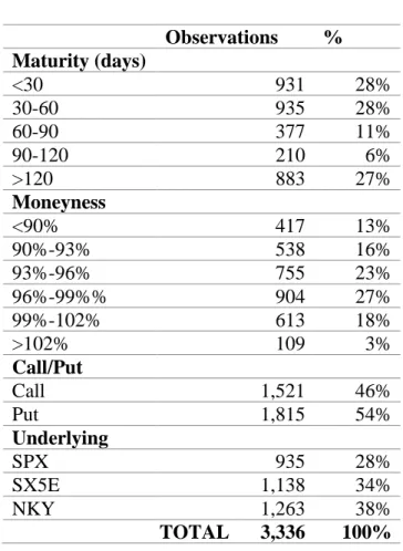
Table 1 – Sample summary Observations % Maturity (days) <30 931 28% 30-60 935 28% 60-90 377 11% 90-120 210 6% >120 883 27% Moneyness <90% 417 13% 90%-93% 538 16% 93%-96% 755 23% 96%-99%% 904 27% 99%-102% 613 18% >102% 109 3% Call/Put Call 1,521 46% Put 1,815 54% Underlying SPX 935 28% SX5E 1,138 34% NKY 1,263 38% TOTAL 3,336 100%

Table 1 presents a summary for the final sample features, regarding its time to maturity, moneyness, option type and underlying.

Due to the liquidity of options on indexes, the sample benefits from good moneyness levels. The reason for the small time to maturity on 56% of the sample happens because the majority indexes options are issued as short-term options. Unlike some empirical papers, this study will include put options.

(32)

24

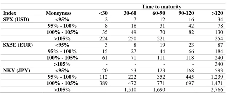
Table 2 summarizes the average quotes per underlying of the observation sample:

Table 2 – Sample average quotes

Time to maturity Index Moneyness <30 30-60 60-90 90-120 >120 SPX (USD) <95% 2 7 12 16 34 95% - 100% 8 16 31 42 78 100% - 105% 35 49 70 82 130 >105% 224 250 221 - 254 SX5E (EUR) <95% 3 8 19 23 87 95% - 100% 15 27 44 66 184 100% - 105% 61 71 111 118 240 >105% - - - - 340 NKY (JPY) <95% 20 53 123 168 593 95% - 100% 112 222 352 445 1,239 100% - 105% 389 472 771 697 1,471 >105% - 1,510 1,690 - 2,766

The overnight LIBOR on each observation day was used as the risk-free rate. The USD LIBOR was used to price SPX options, EUR LIBOR to price SX5E options and JPY LIBOR to price NKY options. Using LIBOR facilitates to standardize the risk-free rate along the three indexes. For the SPX and the NKY, the dividend yield was computed using the respective Total Return indexes (TRI), since these compounds distributed dividends. Since the dividend yield used to price options is on a yearly basis and the TRI accumulate the dividends distributed since the index creation till today, the 2017 dividends had to be computed. For this, the relative difference between the index and its TRI per observation day in 2017 was subtracted to the relative difference in 2018, expelling distributed dividends as follows:

𝐷 = (𝑇𝑅𝐼2018

𝐼₂₀₁₈ − 1) − (

𝑇𝑅𝐼2017

𝐼₂₀₁₇ − 1), (25)

where 𝐼 is the spot price of the index on one observation day and 𝐷 is the annual dividend-yield. For SX5E, since there is no TRI, a similar procedure was used but using EURO STOXX 50 DVP (SX5ED) instead, whose price corresponds to the amount of dividends per share distributed on the year. Since this index is reset around the 11th of December, the dividends

(33)

25

distributed in 2017, from each observation day respectively till the last day before the reset, were summed to the amount of dividends distributed in 2018 till the observation day. Then, having the total amount of dividends per share, this amount was divided by the index price on the observation day, as shown below:

𝐷 =[(𝑆𝑋5𝐸𝐷𝑙𝑎𝑠𝑡 𝑑𝑎𝑦 2017− 𝑆𝑋5𝐸𝐷𝑜𝑏𝑠 𝑑𝑎𝑦 2017) + 𝑆𝑋5𝐸𝐷𝑜𝑏𝑠 𝑑𝑎𝑦 2018]

𝐼₂₀₁₈ . (26)

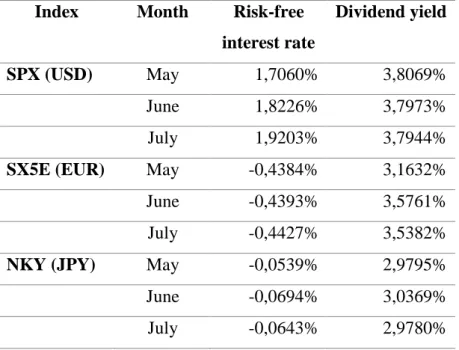
Table 3 details the average for the risk-free interest rates and dividend yields (both annualized) per month used to price the options sample.

Table 3 – Average of the risk-free interest rate and dividend yields

Index Month Risk-free

interest rate

Dividend yield

SPX (USD) May 1,7060% 3,8069%

June 1,8226% 3,7973%

July 1,9203% 3,7944%

SX5E (EUR) May -0,4384% 3,1632%

June -0,4393% 3,5761%

July -0,4427% 3,5382%

NKY (JPY) May -0,0539% 2,9795%

June -0,0694% 3,0369%

(34)

26

3.1. Market brief

3.1.1. SPX

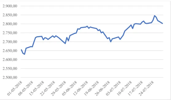
The SPX is showing a very positive performance under the period of analysis, having even reached maximum levels never seen before, as shown in figure IV.

Figure IV – SPX returns

The peak level was reached on the 25th_{of July (2,846 USD) and the lowest level was on the on} the 3rd of May (2,630 USD).

Even with all the “Trump noise” on recent commercial wars like NAFTA fight with Canada, the creation of taxes on imports coming from China, which impacts not only the US but all the world’s economy, as for instance the currency on emerging countries, the confidence for investors on the US stock markets is far away from trembling. The US Federal Reserve has even increased the Fed interest rate from 1,75% to 2% in June this year – where one can see a small decrease on SPX price – which was not enough to scare investors.

2.500,00 2.550,00 2.600,00 2.650,00 2.700,00 2.750,00 2.800,00 2.850,00 2.900,00

(35)

27

Moreover, this thesis witnesses the inverse correlation between volatility and asset returns phenomenon, meaning that, when the asset price goes down the volatility goes up and vice-versa. Using a 30 days sample, the annualized standard deviation of this index is 15% on the 1st of May and 9% on the 30th of July, showing that volatility went down with the rise of the SPX price.

Nevertheless, this significant variation on the index volatility is impacting this empirical work due to the sensitivity of the options pricing to the volatility and underlying returns.

3.1.2. SX5E

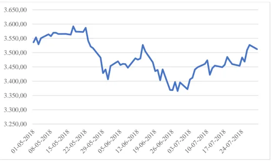
On the other hand, investors’ risk aversion to the Euro Zone is quite notable, as depicted by figure V.

Figure V – SX5E returns

The trade war Europe vs USA mentioned before, the ongoing Greece financial assistance program (during this thesis time period), the “not sure” Brexit, can be some of the reasons for this hesitation from investors.

3.250,00 3.300,00 3.350,00 3.400,00 3.450,00 3.500,00 3.550,00 3.600,00 3.650,00

(36)

28

The highest peak observable is on 17th of May (3,592 EUR), while the lowest is on the 28th of June (3,366 EUR).

The inverse correlation between volatility and index returns is present on SX5E, just like on SPX. The standard deviation floats in a range between 6% and 15% (on a 30-day time gap) where the volatility is higher on the days when this index reached its lowest levels and vice-versa.

3.1.3. NKY

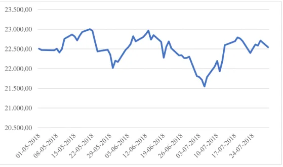
Japan’s economy is not out of this trade tension. A country like Japan, where the exports are one of its most important sources of income, can suffer with this pressure. A constant decrease in production over 2018, due to a lower worldwide demand for Japanese products, has its cost in the economy and NKY shows such issue, as it is possible to observe in figure VI.

Figure VI – NKY returns

Even if one checks the price for NKY on the 1st of May and on the 30th of July and realizes prices are very close of each other, having a look to the graph above, it is straightforward to notice the implicit risk.

20.500,00 21.000,00 21.500,00 22.000,00 22.500,00 23.000,00 23.500,00

(37)

29

The lowest level observed was on the 5th of July (21,547 JPY), while the highest was on the 21st of May (23,002 JPY).

NKY is no exception for the inverse correlation phenomenon stated before, where the volatility started its hike around the 21st of May having an annual standard deviation (again, computed using the last 30-days returns) of 7%, ending the observation period with a volatility of 16%.

3.2. Implicit volatility on the market

Bates (2005) states that, after the 1978 crash, volatility patterns observed in the market do not match what was assumed by the BSM log-normal distribution of returns. This is confirmed on figures VII and VIII, which plots the implicit volatility for the three indexes.

Figure VII – Average of implied volatilities on the three indexes for call options

0% 5% 10% 15% 20% 25% Im p lied v o latilit y Moneyness <30 30-120 >120

(38)

30

Figure VIII – Average of implied volatilities on the three indexes for put options

0% 5% 10% 15% 20% 25% 30% 35% Im p lied v o latilit y Moneyness <30 30-120 >120

(39)

31

4. Empirical results and analysis

Each option pricing model was programmed in MATLAB R2017a 9.2.0.538062 64-bit using a CPU Intel® Quad-core i7 2.60GHz processor with 8 GB RAM. Excel was used to manage and organize the data, so MATLAB could retrieve it and use it on the code. MATLAB would then export the parameter and pricing results back into a new Excel spreadsheet. The programming for the Heston model was based on Rouah (2013).

In this section, the pricing and parameters results will be first detailed and explained by model and secondly results will be compared between the models and a conclusion will be taken. For every model, parameters were estimated using market data and each parameter was estimated on five different ways concerning the time interval for the used data. The time intervals used are: two years; one year; six months; three months and one month. Having five different pricing results per model, only the best results were then investigated.

The best pricing results were chosen based on the performance. Performance was measured using a relative price error (RPE), which is calculated as follows:

𝑅𝑃𝐸 =𝑃𝑡ℎ𝑒𝑜𝑟𝑒𝑡𝑖𝑐𝑎𝑙

𝑃_{𝑚𝑎𝑟𝑘𝑒𝑡} − 1, (27)

where 𝑃𝑡ℎ𝑒𝑜𝑟𝑒𝑡𝑖𝑐𝑎𝑙 corresponds to the theoretical price computed and 𝑃𝑚𝑎𝑟𝑘𝑒𝑡 corresponds to the market close price. Logically, if the RPE is negative (positive), the model is underestimating (overestimating) the benchmark.

After computing RPE for each of the 3,336 observations, this indicator was segmented into different ranges. The parameter estimation which led to the highest weight of observations to fit on the range of -25% to 25% RPE, was considered as the best performance.

RPE was used to compare performances instead of, for instance, an absolute price error (APE) because the indexes under scope have completely different prices and currencies, hence, it would not make sense to compare absolute prices. Bakshi et al. (1997) and Chen et al. (2009) use this method as well. Average of relative pricing errors (ARPE) and absolute average pricing

(40)

32

errors (AARPE, which turns every negative error into positive, to avoid a wrong interpretation applying the average errors) were used in some cases to explain the results.

Next, the results were investigated in Excel.

Finally, results will be analyzed, compared and discussed for each pricing model, after a description of the parameter estimation procedure and results.

4.1. The BSM model

4.1.1. Parameters estimation

One of the eases applying the BSM model is the fact there is only one parameter to estimate, the annualized volatility of the underlying returns 𝜎. The historical volatility was computed in 5 different ways differing on the time interval of data used to compute the standard deviation of the index returns. The annualized standard deviation was computed on time intervals: 2-year, 1-year, 6-month, 3-month and 1-month.

Previous literature uses averages of implied volatilities (see for example Bakshi et al. (1997), Jackwerth and Rubinstein (2012) or Chen et al. (2009)) to compute the BSM volatility to apply on its pricing. This method is much more expensive than the historical volatility because one needs to use much more data to segment the options into strike prices and time to maturity due to the volatility smile.

(41)

33

Next, the volatility behavior analysis over the observations period on each index is shown in figures IX, X and XI.

Figure IX – SPX volatility

Regarding the SPX, the index with the best performance, the short-term volatilities are the flattest of the three indexes. With a steady curve, the 1-month and 3-month volatilities are decreasing as the index prices keep rising.

Figure X – SX5E volatility

0% 5% 10% 15% 20% 25%

2-year volatility 1-year volatility 6-month volatility

3-month volatility 1-month volatilty

0% 2% 4% 6% 8% 10% 12% 14% 16% 18%

(42)

34

With respect to SX5E it is possible to notice that when the index returns are positive the volatility reaches its minimum levels, while when the index returns start to decline, the volatility starts its hike. As expected, volatilities computed with larger data samples are steadier than with smaller data samples.

Figure XI – NKY volatility

The NKY has the particularity of having big volatility levels on the index prices during the observation period, but at the same time only moved 0,16% from the 1st_{of May to the 30}th_of July. Even though, one can see that the 1-month volatility is constantly rising up even when the stock returns are positive, maybe because, in this case, the index price was so volatile that surpassed the inverse correlation impact.

Generally, as expected, one can conclude that with bigger time gaps the volatility tends to become flat, while with smaller time gaps each significant variation has a bigger impact on the standard deviation. Thus, the 2-year, 1-year and even 6-month volatility are quite flat, while the 3-month and 1-month volatility have some peaks among the three indexes. One interesting fact is that the 3-month volatility in all indexes have the same trend, where the volatility level drops from the 1st of May to the 30th of July.

0% 5% 10% 15% 20% 25%

(43)

35

4.1.2. Pricing analysis

The pricing errors were computed for each time gap and the 2-year historical volatility showed the best performance for the BSM. This may be due to, as seen before, the 2-year volatility being the most consistent. Hereafter, the presented figures respect to the computations using 2-year volatility.

Table 4 – BSM RPE segment

Error % <-75% 15% [-75%; -50%[ 7% [-50%; -25%[ 11% [-25%; 0%[ 20% [0%; 25%[ 21% [25%; 50%[ 9% [50%; 75%] 4% >75% 13% TOTAL 100%

Table 4 segments the RPE between the market and the theoretical price obtained with the BSM. As one can see, 41% of the options are on the error range of -25% to 25%. About half of the sample is between an error of -50% and 50%. It is also important to notice the weight of the tails, where 28% of the sample has a RPE higher than 75% or lower than -75%.

Table 5 – BSM performance - AARPE

Moneyness Time to maturity (days) TOTAL

<30 30-60 60-90 90-120 120-150 >150 <90% 96% 100% 99% 149% 52% 50% 84% 90% - 93% 117% 141% 67% 81% 63% 26% 93% 93% - 96% 123% 104% 60% 51% 33% 18% 84% 96% - 99% 68% 55% 31% 16% 24% 13% 46% 99% - 102% 30% 27% 15% 16% 19% 17% 23% >102% 14% 18% 16% 18% 12% 16% 16% TOTAL 82% 83% 50% 48% 33% 24% 61%

(44)

36

Figure XII – BSM performance - ARPE

Table 5 represents the BSM performance measured on AARPE over the time to maturity and moneyness. It is demonstrated that BSM has a much better behavior when pricing ATM and ITM options, where AARPE is 23% and 16%, respectively. This is also plotted in figure XII, which shows the performance measured on ARPE, where the green and light blue curves are much more consistent (range between -11% and 22%) and closer to 0 as the time to maturity increases.

On deep OTM and OTM options (dark blue and orange line, respectively) the curves reveal big oscillations (range between -95% and 57% for ARPE) along the maturity. Table 5 supports that statement, where AARPE is 84% and 93%. It also shows that when options are reaching maturity its performance following the market is weaker than when the time to maturity is larger, where on this last case even OTM options lean to a lower ARPE. This conclusion goes alongside with Bakshi et al. (1997) empirical results.

Bakshi et al. (1997) also state that, generally, option pricing models overprices OTM and underprices ITM call options. Empirical results of this thesis confirm such observation.

<30 30-60 60-90 90-120 120-150 >150 <90% -95% -40% -36% 57% -40% 10% 90%-93% -31% 51% -8% 22% 20% -1% 93%-96% 21% 49% 30% 32% 17% -3% 96%-99% 30% 43% 20% 11% 16% -3% 99%-102% 21% 22% 3% 5% 7% -4% >102% 7% 11% 0% 2% 2% -11% -120% -100% -80% -60% -40% -20% 0% 20% 40% 60% 80% A R P E

Time to maturity (days)

<90% 90%-93% 93%-96% 96%-99% 99%-102% >102%

(45)

37

Table 6 – BSM RPE segment for call options - Moneyness

RPE Moneyness TOTAL

<95% 95%-97% 97%-99% 99%-101% >101% <-25% 5% 1% 1% 2% 2% 12% [-25%; 0%[ 3% 2% 3% 3% 11% 23% [0%; 25%[ 3% 2% 4% 4% 4% 17% [25%; 50%] 3% 2% 4% 2% 1% 12% >50% 19% 10% 7% 1% 0% 37% TOTAL 33% 18% 20% 11% 18% 100%

Table 7 – BSM RPE segment for call options – Time to maturity

RPE Time to maturity (days) TOTAL

<30 30-60 60-90 >90 <-25% 3% 1% 1% 7% 12% [-25%; 0%[ 4% 4% 2% 13% 23% [0%; 25%[ 4% 5% 2% 7% 17% [25%; 50%] 3% 3% 2% 3% 12% >50% 11% 16% 4% 6% 37% TOTAL 25% 28% 11% 36% 100%

Tables 6 and 7 segment the pricing errors by moneyness and time to maturity for the observed call options. 49% of this sample is overpriced (RPE between 25% and >50%) and around 12% underpriced (RPE <-25%).

34% of call options are overpriced and OTM (moneyness <97%), whereas 2% are underpriced and ITM (moneyness above 101%).

Regarding the time to maturity, BSM seems to overprice call options near the maturity (33% is reaching maturity in less than 60 days and has RPE above 25%) while 7% is underpriced and have a time to maturity higher than 90 days.

Summarizing, BSM overprices call options when OTM or reaching maturity, while underprices ITM options or with a longer time to maturity. BSM shows to be very sensitive to moneyness and time to expiration.

(46)

38

Table 8 – BSM RPE segment for put options - Moneyness

RPE Moneyness TOTAL

<95% 95%-97% 97%-99% 99%-101% >101% <-25% 40% 8% 3% 0% 0% 51% [-25%; 0%[ 7% 4% 4% 1% 1% 18% [0%; 25%[ 4% 3% 7% 5% 4% 23% [25%; 50%] 0% 2% 2% 1% 1% 6% >50% 0% 0% 1% 0% 0% 1% TOTAL 51% 17% 17% 8% 7% 100%

Table 9 – BSM RPE segment for put options – Time to maturity

RPE Time to maturity (days) TOTAL

<30 30-60 60-90 >90 <-25% 21% 17% 6% 7% 51% [-25%; 0%[ 3% 4% 2% 10% 18% [0%; 25%[ 3% 4% 3% 13% 23% [25%; 50%] 2% 3% 1% 1% 6% >50% 1% 0% 0% 0% 1% TOTAL 30% 28% 12% 30% 100%

Tables 8 and 9 segment the pricing errors for put options by moneyness and time to maturity, respectively for put options. 51% of this sample is underpriced while only 7% is overpriced. As one can see, the BSM tends to underprice put options reaching maturity or deep OTM options more often. It is not clear to see when the BSM overprices put options because the percentage of overpricing is very small (around 7%).

There is a big performance gap on the BSM depending on the options moneyness and time to expiration, also argued by Bakshi et al. (1997). BSM shows to be very sensitive to when time to expiration is below 90 days, where independently from the moneyness, errors have a big oscillation. In addition, when options are ATM or ITM, BSM behaves reasonably well.

(47)

39

4.1.3. Implied volatility

Figures XIII and XIV show the implied volatility of the computed prices using the BSM model.

Figure XIII – Average of implied volatilities for the BSM model on the three indexes for call options

Figure XIV – Average of implied volatilities for the BSM model on the three indexes for put options

0% 2% 4% 6% 8% 10% 12% 14% 16% 18% Im p lied v o latilit y Moneyness <30 30-120 >120 0% 2% 4% 6% 8% 10% 12% 14% 16% Im p lied v o latilit y Moneyness <30 30-120 >120

(48)

40

It is clear to see that the implied volatilities taken from the computed prices using the BSM model, where the volatility used is based on historical returns, are not in line with the market. This supports previous researches when it is argued that the assumptions under the BSM model are not the most coherent with the markets.

4.2. The CEV model

4.2.1. Parameters estimation

As mentioned in chapter 1, the RMSRE method was applied in order to estimate the two parameters not observable in the market for the CEV model: 𝛽 and 𝛿. The optimal 𝛽∗_is computed assuming equation (6.4) for 𝛿̃(𝛽). Afterwards, equation (6.4) is used again to retrieve the optimal 𝛿∗_{using 𝛽}∗_.

Inspection of equation (6) shows that the application of the CEV formula is dependent on 𝛽 (if 𝛽 is lower, higher or equal 2). A disadvantage for this method is the time required to estimate 𝛽∗_.

On MATLAB, each 𝛽∗ was estimated twice, using both formulas presented on equation (6) for call options and (7) for put options, to understand if this parameter should be higher or lower than 2. After running the routine several times assuming 𝛽 > 2, it was possible to observe that the function was always leaning for the lower boundary of 2.5 (the estimated 𝛽 was most of the times equal to 2.5), so it was easy to conclude that 𝛽 < 2 was the right path, meaning, the instantaneous volatility is inversely correlated with the index price2, as shown before.

Chen et al. (2009) and Jackwerth and Rubinstein (2012) concluded that computing the parameter 𝛽 without restrictions would provide better results than if this parameter is restricted. The only restriction to compute 𝛽 on this thesis was an upper boundary of 1.5 so 𝛽 would not approximate 2 (BSM case).

2_{The time to price 3,336 options observations with CEV model using β>2 was around 1 hour, due to complex}

(49)

41

For 𝜎, the same procedure as for the BSM was applied. This means, 𝛽 and 𝛿 were estimated 5 times for every observation using different historical volatility time gaps. The price for every observation was also computed 5 times, in order to compare the performances.

Table 10 – Average of estimated 𝜷

Index Volatility time gap

1-month 3-month 6-month 1-year 2-year

SPX -19,33 -17,66 -14,60 -16,11 -18,21 (11,74) (7,78) (3,61) (4,92) (11,23) SX5E -19,46 -9,87 -10,81 -10,09 -10,14 (16,49) (5,62) (3,82) (7,34) (5,45) NKY -11,77 -3,91 -8,40 -5,84 -7,05 (18,05) (4,94) (2,38) (2,9) (3,01)

Table 10 shows the average estimations and standard deviation (in parentheses) for 𝛽 per underlying, for each volatility time gap.

As expected, the standard deviation for estimated 𝛽 is much higher for smaller time gaps than for larger time gaps. This might be, again, due to consistency on larger volatility time periods, even though the 2-year time gap is below expectations.

Another point of interest is the difference between 𝛽 on the 3 indexes. Even having the SPX with the lowest 𝛽, this shows to be the most consistent over all the volatility time gaps used. In contrast with Jackwerth and Rubinstein (2012), which shows the post-crash of 1987 𝛽 should be around -6, the average 𝛽 estimated on this study for SPX is in between -15 and -19. This discrepancy can happen due to inverse correlation between asset prices and volatility, where SPX, as shown before, is reaching high levels (decreasing the volatility) as never seen before, increasing the elasticity for the volatility.

Having such large 𝛽, the estimated values for 𝛿 are enormous (most of the times the value is higher than 1010_).

(50)

42

4.2.2. Pricing analysis

Not as expected, the CEV model shows the best performance using a volatility time gap of 1 year, even though it did not outperform considerably comparing with 2-year time gap (4% difference). Hereafter, all figures respect to the 1-year volatility computations.

Table 11 – CEV RPE segment

Error % < -75% 11% [-75%; -50%[ 9% [-50%; -25%[ 15% [-25%; 0%[ 24% [0%; 25%[ 25% [25%; 50%[ 11% [50%; 75%] 3% >75% 2% TOTAL 100%

Table 11 segments the RPE of the pricing computation under the CEV model. Almost half of the sample is on the RPE of -25% to 25%, which seems, at first sight, to outperform BSM.

Table 12 – CEV performance - AARPE

Moneyness Time to maturity (days) TOTAL

<30 30-60 60-90 90-120 120-150 >150 <90% 92% 55% 45% 44% 31% 55% 60% 90% - 93% 81% 40% 27% 37% 35% 41% 48% 93% - 96% 52% 27% 21% 25% 22% 25% 33% 96% - 99% 42% 29% 21% 17% 16% 18% 29% 99% - 102% 25% 19% 16% 18% 11% 17% 19% >102% 4% 6% 13% 14% 5% 17% 13% TOTAL 51% 32% 24% 25% 20% 29% 35%

(51)

43

Figure XV – CEV performance - ARPE

Table 12 shows the CEV performance measured on AARPE over the time to maturity and moneyness. Similar to the BSM, the CEV model has a better performance when pricing ATM and ITM options, as well as options with a longer time to expiration. The AARPE for the total sample reaches 35%, which illustrates a very good performance. The best performance disregarding moneyness level is when options have a time to maturity between 60 and 120 days where AARPE is 24% for 60-90 days to maturity and 25% for 90-120 days to maturity. Figure XV illustrates it, where one can see all curves lean to 0% ARPE when time to expiration is around 60 and 120 days, having the 4 curves with moneyness higher than 93% very close to 0. Even though, OTM curves still oscillate before for low maturity options. Nevertheless, every moneyness tends to a ARPE of 0 when maturity rises.

Splitting this performance between call and put options, an interesting result happens.

Table 13 contains the AARPE by kind of option. Results show that the CEV model seems to fit better the market computing options with higher maturities when these are put options rather than call options. When maturity >150 days, call options have an AARPE of 42%, while put

<30 30-60 60-90 90-120 120-150 >150 <90% -92% -48% -16% -12% 22% -34% 90%-93% -81% -32% -12% -17% -12% -25% 93%-96% -43% 0% -7% -4% -14% -17% 96%-99% 16% 20% 4% -2% -10% -13% 99%-102% 14% 12% 5% 1% -3% -14% >102% -2% -4% -2% 1% -3% -15% -100% -80% -60% -40% -20% 0% 20% 40% A R P E

Time to maturity (days)

<90% 90%-93% 93%-96% 96%-99% 99%-102% >102%

(52)

44

options show 33%). There is no evidence to distinguish the performance between call and put options regarding its moneyness, since both have better performances on ITM zone, as said before.

(53)

45

Table 13 - CEV performance by option kind - AARPE

Moneyness

Call options

TOTAL

Put options _{TOTAL TOTAL}

Time to maturity (days) Time to maturity (days)

<30 30-60 60-90 90-120 120-150 >150 <30 30-60 60-90 90-120 120-150 >150 <90% 100% 76% 47% 84% 70% 77% 76% 91% 49% 44% 32% 29% 34% 54% 60% 90%-93% 81% 45% 22% 46% 57% 60% 53% 80% 37% 30% 32% 22% 23% 45% 48% 93%-96% 47% 29% 21% 28% 28% 46% 35% 55% 26% 20% 21% 16% 12% 32% 33% 96%-99% 54% 34% 24% 20% 24% 33% 38% 31% 23% 17% 14% 8% 7% 21% 29% 99%-102% 25% 19% 14% 15% 12% 25% 21% 25% 19% 18% 20% 9% 5% 17% 19% >102% 4% 6% 15% 15% 6% 18% 15% 4% 6% 10% 12% 5% 4% 7% 13% TOTAL 47% 33% 22% 27% 25% 42% 37% 54% 30% 26% 23% 16% 16% 33% 35%