Building Neural Net Software
João Pedro Neto
José Félix Costa
DI-FCUL
TR–99–5
December 1999
Departamento de Informática
Faculdade de Ciências da Universidade de Lisboa
Campo Grande, 1700 Lisboa
Portugal
Technical reports are available at
http://www.di.fc.ul.pt/biblioteca/tech-reports
. The files are stored in PDF, with the report number as filename.
Alternatively, reports are available by post from the above address.
Building Neural Net Software
*
J. Pedro Neto and J. Félix Costa
{jpn, fgc}@di.fc.ul.pt
Faculdade de Ciências da Universidade de Lisboa
Bloco C5 - Piso 1, 1700 Lisboa, PORTUGAL
Abstract. In a recent paper [Neto et al. 97] we showed that programming languages can be
translated on recurrent (analog, rational weighted) neural nets. The goal was not efficiency
but simplicity. Indeed we used a number-theoretic approach to machine programming,
where (integer) numbers were coded in a unary fashion, introducing a exponential slow
down in the computations, with respect to a two-symbol tape Turing machine.
Implementation of programming languages in neural nets turns to be not only theoretical
exciting, but has also some practical implications in the recent efforts to merge symbolic
and subsymbolic computation. To be of some use, it should be carried in a context of
bounded resources. Herein, we show how to use resource boundedness to speed up
computations over neural nets, through suitable data type coding like in the usual
programming languages. We introduce data types and show how to code and keep them
inside the information flow of neural nets. Data types and control structures are part of a
suitable programming language called
NETDEF. Each
NETDEFprogram has a specific neural
net that computes it. These nets have a strong modular structure and a synchronisation
mechanism allowing sequential or parallel execution of subnets, despite the massive
parallel feature of neural nets. Each instruction denotes an independent neural net. There
are constructors for assignment, conditional and loop instructions. Besides the language
core, many other features are possible using the same method. There is also a
NETDEFcompiler, available at www.di.fc.ul.pt/~jpn/netdef/netdef.htm.
1.
Introduction
Analog recurrent neural nets can be formulated as dynamic systems. We adapt to
our case the definition given in [Sontag 90], that corresponds to the concept of
discrete, complete, time-invariant dynamic system. A dynamic system is a triple
D = (S, U,
φ
) consisting of: (a) a non-empty set S called the state space of D, (b) a
non-empty set U called the control-value or input-value space of D, and (c) a total
map called the dynamic map,
φ
: S
×
U
→
S. We will consider S and U as being finite
dimensional vector spaces over the reals, or restrictions to them.
Analog neural nets are considered particular cases of dynamic systems, where
φ
is
of the form
σ°π
, being
π
: S
×
U
→
S an affine map, and
σ
: S
→
S a possibly
discontinuous function. Linearity of
π
is equivalent to the existence of linear maps
A: S
→
S and B: U
→
S such that
φ
(x,u) =
σ
(Ax+Bu). These systems are said to be
autonomous whenever B is the null matrix, otherwise they are said to be
non-autonomous or net systems with controls. If we assume that there exists one
variable with constant value 1, and specific matrices, we recover the model in the
form
φ
(x,u) =
σ
(Ax+Bu+c), where c is known as the bias vector.
We will consider two cases for the function
σ
:
(a) the McCulloch and Pitts neural net model,
σ
(x)
=
0 if
x
<
0
1 if
x
≥
0
(b) the saturated sigmoid model,
σ
(x)
=
0 if
x
<
0
x if
0
≤
x
≤
1
1 if
x
>
1
(1)
For notational purposes we write
x(t+1) =
φ
( x(t), u(t) )
(2)
to denote a step of computation, or just
x
+=
φ
( x, u )
With dynamical systems in general we have computation without programmability,
i.e., the extra power these systems exhibit has to do with the decoupling between
programming and computation. Up to the power of Turing machines, computations
are describable by programs that correspond to the prescription by finite means of
some rational parameters of the system. Beyond Turing power we have
computations that are not describable by finite means: computation without a
program. In this paper we want to shed some light on the programmability of
neural nets.
1.1.
Computability
The use of an analog neural net model in computability is due to Hava Siegelmann
and Eduardo Sontag. In [Siegelmann and Sontag 95] they used it to establish lower
bounds on the computational power of analog recurrent neural nets.
These systems satisfy the classical constraints of computation theory, namely, (a)
input is discrete (binary) and finite, (b) output is discrete (binary) and (c) the
system is itself finite (control is finite). Neurons may hold values within [0,1] with
unbounded precision. To work with such analog systems, binary input is encoded
into a rational number between 0 and 1, and the rational output is decoded into an
output binary sequence.
The input streams u
k, for i=1..M, input bits into the system through time. Streams
are maps u
k:
→
{0,1}, different from 0 only finitely many times (this is the
classical constraint of input finiteness). (u
k)
k=1..M, is the set of control symbols, to
adopt the flavour of Minsky's description of such systems, that the reader may find
in [Minsky 67]. In the absence of control the systems are said to be autonomous
and the dynamics is given by
x
j
(t+1) =
σ
(
∑
i=1
N
a
ji
x
j
(t) + c
j
)
We may then identify the set of computable functions by analog recurrent neural
nets, provided that the type of the weights is given. This research program has been
systematically pursued in [Siegelmann 99]:
•
The first level of nets is NET[integer], where the type of the weights is integer.
These nets are historically related with the work of Warren McCulloch and
values are thus always zero or one. Thus in the case of integer nets the
activation function can be replaced by the Heaviside step function with no
decrease (or increase) of computational power. In this case the nets
'degenerate' into a classical devices called finite automata. It was Kleene who
first proved that McCulloch and Pitts' nets are equivalent to finite automata,
and therefore they were able to recognize all regular languages (see [Minsky
67] for details).
•
The second relevant class we consider in this paper is NET[rational], where
the type of the weights is rational. Rationals are indeed computable numbers in
finite time, and NET[rational] turn to be equivalent to Turing machines.
Twofold equivalent: rational nets compute the same functions as Turing
machines and, under appropriate coding of input, they are able to compute the
same functions in exactly the same time.
•
The third relevant class is NET[real], not considered in this paper, where the
type of the weights is real. Reals are indeed in general non computable. But
theories of physics consider real variables. The advantage of making an analog
theory of computation is that non uniform classes of computation, namely the
classes that arise in complexity theory using Turing machines with advice, are
uniformly described in NET[real]. All sets over finite alphabets can be
represented as reals that encode the families of Boolean circuits that recognize
them. A further feature is that, if we allow only for computable reals, then we
can develop a model that is strictly as powerful as Turing machines, but with
the computations being speed up by exponential factors. The reason is that the
complexity of computable reals have no upper limit. In classical artificial
devices, these constants have to be calculated with the required precision,
slowing down the computations.
1.2.
Programmability of Analog Neural Nets
Within the class of NET[rational] we can develop the implementation of
programming languages, providing for each written command, a suitable analog
neural net. The implementation map will be provided in this paper for a (Turing
complete) subset of the Occam language.
A first concern is the size of the resulting nets. In fact the size of the nets will
increase with the complexity of programs. However, is always possible to
implement the Occam interpreter of Occam, determining a universal neural net for
the language interpretation.
We see two main contributions in this paper. In first place, we show how to
perform symbolic computations over neural nets. And in second place, the
high-level programming language is useful for high-level construction of particular
nets, used in the proof of several results in neurocomputing theory, as in
[Siegelmann 99], where a net descriptor is used to encode analog shift maps into
neural nets.
2.
Neural Software
2.1.
Neural Net Model
An analog recurrent neural net is a dynamic system x
→
(t+1) =
φ
( x
→
(t), u
→
(t)), with
initial state x
→
(0) = x
→
0, where x
i
(t) denotes the activity (firing frequency) of neuron
i at time t within a population of N interconnected neurons, and u
k
(t) the input bit
of input stream k at time t within a set of M input channels. The application map
φ
is taken as a composition of an affine map with a piecewise linear map of the
interval [0,1], known as the saturated sigmoid
σ,
as in (2). The dynamic system
becomes
x
j(t+1) =
σ
(
∑
i=1
N
a
jix
i(t) +
∑
k=1
M
b
jku
k(t) + c
j)
where a
ji
, b
jk
and c
j
are rational weights, assuring that a system can be simulated by
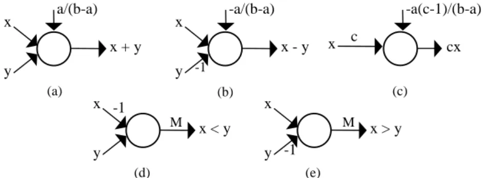
a Turing machine. Fig. 1 displays the graphical representation of the preceding
equation used throughout this paper (when a
ji, b
jkor a
jjtakes value 1, they are not
displayed in the graph.).
Fig. 1. Graphical notation for neurons, input channels and their interconnections.
Our problem will be to find a suitable neural network for each program written in
the chosen programming language.
2.2.
The NETDEF Language
We will adopt a fragment of Occam
®for the programming language. Occam
®was
designed to express parallel algorithms on a network of processing computers (for
more information, see [SGS-T
HOMSOM
95]). With this language a program can be
described as a collection of processes executing concurrently, and communicating
with each other through channels. Processes and channels are the main concepts of
the Occam
®programming paradigm.
Occam
®programs are built from processes. The simplest process is an action.
There are three types of action: assignment of an expression to a variable, input and
output. Input means to receive a value from a channel and assign it to a variable.
Output means to send the value held by a variable through a channel.
There are two primitive processes: skip and stop. The skip starts, performs no
action and terminates. The stop starts, performs no action and never terminates. To
construct more complex processes, there are several types of construction rules.
Herein, we present some of them: while, if, seq and par.
The if is a conditional construct that combines a number of processes, guarded by a
boolean expression. The while is a loop construct, that repeats a process while an
associated boolean expression is true. The seq is a block construct, combining a
a
jjc
ja
jix
ix
ju
kA communication channel provides unbuffered, unidirectional point-to-point
communication of values between two concurrent processes. The format and type
of values are defined by a certain specified protocol.
Here follows the simplified grammar of
NETDEF
(Network Definition), in EBNF:
program ::= “
NETDEF” id “
IS” def-var process “.”.
process ::= assignment | skip | stop | if-t-e | while-do | seq-block | par-block.
Our goal is to show that all
NETDEF
programs are compiled into neural nets. There
exists a dynamic system of the kind (3) that runs any
NETDEF
program on some
given input.
2.3.
Information Coding and Operators
With the guidelines provided in
[
Siegelmann
96
]
, the seminal work on the
implementation of information coding in neural networks (see
[
Gruau et al. 95
]
for
a different approach), we introduce data types and show how to encode and keep
them inside the information flow of neural nets.
NETDEF
has the following type
definitions.
type ::= primitive-type | channel-type | composite-type.
primitive-type ::= “
BOOLEAN” | “
INTEGER” | “
REAL”.
channel-type ::= “
CHANNEL”.
composite-type ::= “
ARRAY” “[“ number “]” “
OF” primitive-type.
2.3.1. Primitive Types
To be of some use, implementation of programming languages in neural nets
should be carried in a context of bounded resources. Herein we show how to use
resource boundedness to speed up computations over neural nets, through suitable
encoding of suitable data types like in the usual programming languages.
To take in consideration the lower and upper saturation limits of the activation
function
σ
, every value x of a given basic type is encoded into some value of
[
0,1
]
.
For each type T, there is an injective encoding map
α
T:T
→[
0,1
]
mapping a value
x
∈
T onto its specific code. The encoding map determines the operator neural
architecture. Basic types include: boolean, integer and real.
If resources are bounded, then there exists a limit to the precision of every value (in
fact, even reals are bounded rationals). Suppose a maximum precision of P digits.
The minimum distance between any two values is 10
-P. Let us denote
10
Pby M.
For booleans, T is B = {0,1}, the encoding map is given by
α
B(x) =
0 , x=
FALSE
For integers, T is Z = { -
M
2
,
M
2
}, and
α
Z(x) =
M + 2x
2M
For reals, within
[
a,b
]
,
α[
a,b](x) =
x-a
b-a
2.3.2. Channel and Composite Types
Each channel has two neurons, one to keep the processed value and another neuron
to keep a boolean flag (with value one if the channel is empty, or zero, otherwise).
To see more about channels see section 2.4.2.
It is also possible to define array variables. Each one of the data elements is coded
by a specific neuron. This means that a composite type is a finite set of neurons.
The array has the following structure,
Fig. 2. An array basic structure.
2.3.4. Operators
With data types, many different operators are needed to process information. An
arbitrary set of operators (together with constants, variables and input data) forms
an expression that after evaluation returns a result of some type. Each expression
starts its execution when it receives signal
IN
(for details see section 2.4.1). After
evaluation, it returns the final result through output
RES
at the same time of signal
OUT
.
Fig. 3. An expression subnet.
Non-labelled arcs default to weight 1.
•
Boolean Operators. These are the typical McCulloch-Pitts boolean operators
(see
[
McCulloch and Pitts 43
]
)
Fig. 4. Boolean Operators: (a)
NOT X, (b)
X AND Y, (c)
X OR Y.
OUT Expr RES IN (a)
x
¬
x
1
-1
(b)x
y
x
∧
y
-1
(c)x
y
x
∨
y
• Integer Operators. There are arithmetical and relational operators for integers.
Fig. 5. Integer Operators: (a) -
X, (b)
X+
Y, (c)
X-
Y, (d)
X<
Y, (e)
X>
Y.
• Real Operators. The encoding α
[a,b]is a scaling of the interval
[
a,b
]
into
[
0,1
]
.
Binary sum, subtraction and multiplication by a constant are straightforward.
Fig. 6. Real Operators: (a)
X+
Y, (b)
X-
Y, (c) c
X, (d)
X<
Y, (e)
X>
Y.
2.4.
Synchronization Mechanisms
Neural nets are models of massive parallelism. At each instant, all neurons are
updated, possibly with new values. This means that a network step with n neurons
is a parallel execution of n assignments. Since programs (even parallel programs)
have a sequence of well-defined steps, there must be a way to control it. This is
done by a synchronization mechanism based on hand-shaking.
2.4.1. Instruction Blocks
There are two different ways to combine processes, the sequential block and the
parallel block. Each process in a sequential block must wait until the previous
process ends its computation. In a parallel block each process starts at the same
time, independently of the others. But the parallel block (which is itself an process)
only ends when all processes terminate. This semantic demands synchronisation
mechanisms in order to control the intrinsic parallelism of neural nets.
To accomplish this, each
NETDEF
process has a specific and modular subnet
binding its execution and its synchronization part. Each subnet is activated when
the value 1 is received through a special input validation line
IN
. The computation
of a subnet terminates when the validation output neuron
OUT
writes value 1.
OUT IN
IN
I
1 OUT...
I
2 INI
nOUT
(a) (a)x
-x
1
-1
(b)x
y
x + y
(c)x
y -1
x - y
(d)x
y
x < y
(e)x
y
M M-1
-1
x > y
-1/2
1/2
cx
(a) (b)x
y
x + y
(c)x
y
-1x - y
(d)x
y
x < y
(e)x
y
M M-1
-1
x > y
c
x
-a/(b-a)
a/(b-a)
-a(c-1)/(b-a)
Fig. 7. Block Processes: (a)
SEQ I1, …,
In ENDSEQ,
(b)
PAR I1, …,
In ENDPAR. All subnets are denoted by squares.
2.4.2. Occam
®Channels
NETDEF
assumes the Occam
®channel communication protocol, allowing
independent process synchronisation.
We introduce two new processes,
SEND
and
RECEIVE
.
send ::= “
SEND” id “
INTO” id.
receive ::= “
RECEIVE” id “
FROM” id.
SEND
sends a value through a channel, blocking the process if the channel is full,
and
RECEIVE
receives a value through the channel, blocking if the channel is empty,
and waiting until something arrives. To minimise the blocking nature of channels,
see sections 2.7 and 2.8.
Fig. 8. Channel Instructions: (a)
VARC:
CHANNEL, (b)
SEND X INTO C(c)
RECEIVE Y FROM C.
Each channel has a limited memory of one slot. Using several channels in
sequence, it is possible to create larger buffers. For e.g.,
SEQ
RECEIVE X
1
FROM C1;
SEND X1
INTO C-
TEMP;
RECEIVE X2
FROM C-
TEMP;
SEND X2
INTO C2;
ENDSEQ;
simulates a buffer with two elements.
(b) OUT OUT OUT
-(n-1)
-1
-1
-1
-1
IN
I
2OUT
I
1I
n...
C
C
e? (a)C
C
e?X
IN-1
2
-2
-1
-1
OUT-1
wait (b) (c) INC
C
e?Y
-1
-1
OUT wait-1
-2
-1
-1
2.4.3. Shared Variables
Processes may communicate through global variables - variables defined on the
initial block. In principle, each neuron could see every other neuron in the net. The
subject of variable scope is an a-priori restriction made by the compilation process.
Several methods in literature, like semaphores or monitors, are implemented as
primitive instructions. These methods are used to promote mutual exclusion
proprieties to a certain language, helping the programmer to solve typical
concurrent problems. In
NETDEF
there is also a mutual exclusion mechanism for
blocks, providing the same type of service.
2.5.
Control
NETDEF
Structure
The control structure of a
NETDEF
program consists of one block process (
SEQ
or
PAR
). This process denotes an independent neural net as seen before. The
implementation is then recursive, because each process might correspond to a set of
several processes. The process subnets are built in a modular way, but they may
share information (via channels or shared variables).
Besides the
IN
and
OUT
synchronization mechanism explained in 2.4.1, there is a
special reset input for each instruction module. This reset is connected to every
neuron of the subnet instruction with weight -1. So, if the signal one is sent through
this channel, all neuron activation terminates on the next instant. For simplification,
we do not show these connections. Once more, all subnets are denoted by squares
and non-labelled arcs default to weight 1.
Fig. 9. Skip and Stop processes: (a)
SKIP, (b)
STOP.
Fig. 10. Assignment Process:
A:=
EXPR. All subnets are denoted by squares.
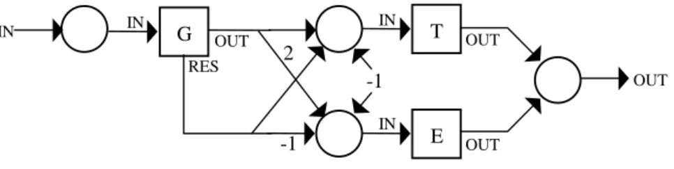
Fig. 11. Conditional Process:
IF G THEN T ELSE E. All subnets are denoted by squares.
IN OUT IN (b) (a) OUT
-1
-1
IN IN Expr OUT RESA
OUT OUT OUT-1
2
-1
IN OUTG
IN IN IN REST
E
The
CASE
process can be seen as the parallel block of
IF
processes. The
COND
process is the sequential block of
IF
processes.
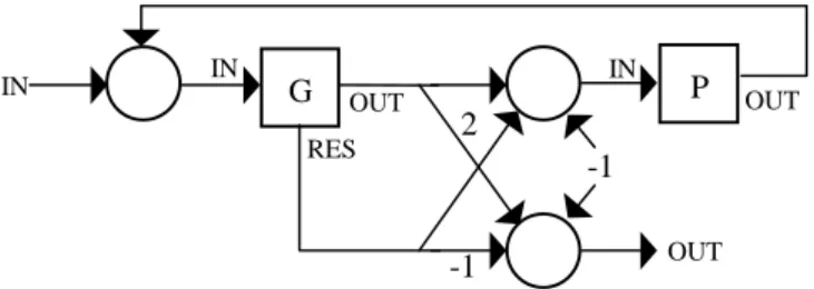
Fig. 12. Loop Instruction:
WHILE G DO P. All subnets are denoted by squares.
Other loop instructions (like
REPEAT
-
UNTIL
) are built in the same way.
2.6.
Procedures and Functions
Functions and Procedures are not duplicated. They have complex neural nets to
ensure that just one call is executed at each time, blocking other calls until the end
of execution. This make effective lock mechanisms on shared data (e.g., accessing
data through only one procedure).
Functions and procedures have parameters by value (copy the value of the
expression into the argument of the procedure/function) and a sort of parameter by
result (copy the value of the variable into the argument and when the
function/procedure ends, copy the value of the argument back to the initial
variable). For syntax details see example in 3.2.
However, an important fault exists in
NETDEF
functions and procedures, there is no
recursion. This is a complex problem, since the number of neurons is fixed by
compilation. There is no easy way to simulate a stack mechanism of function calls
into neural nets.
2.7.
Input / Output
To handle input from the environment and output results,
NETDEF
uses the channel
primitives with two special set of channels,
IN
k(linked directly with input
channel u
k) and
OUT
k. The number of in/out channels is defined before compilation.
This subject depends on the application context, so we do not define the
architecture of these interfaces. In principle, input channels must have a FIFO list
in order to keep the incoming data, and a structure to maintain the
IN
kchannels in a
coherent state (i.e., update the channel flag of
IN
keach time u
ksends a value).
Fig. 13. Input channel u
kconnects with
NETDEFchannel
INk.
With these, in/out operations are simple channel calls. An in/out example could be,
SEQRECEIVE
a
FROM IN1;
SENDa
INTO OUT2;
ENDSEQ;
OUT OUT OUT-1
2
-1
IN ING
IN RESP
IN
ku
kTo obtain asynchronous in/out, there is a boolean function
IS
E
MPTY
(channel)
returning true if the channel is empty, or false otherwise.
Fig. 14. Asynchronous in/out.
E.g., to implement an asynchronous output,
IF ISE
MPTY(
C)
THEN SEND X INTO C2.8.
Timers
In real applications, some processes may create deadlock situations. The
NETDEF
communication primitives (
SEND
and
RECEIVE
) are blocking, i.e., they wait until
some premises are satisfied (the channel must be empty for
SEND
and full for
RECEIVE
). The problem lies if these premises never happen. And waiting
indefinitely for input can be a serious problem in real-time applications. To handle
this,
NETDEF
has several timer processes.
The first one is
TRY
. It guarantees termination, if the instruction does not end
before the expected time (given by an integer variable).
timed-instruction ::= “
TRY” “(“ variable ”)” instruction.
Fig. 15. Timer Constructor:
TRY(
N)
P. All subnets are denoted by squares.
neurons X has arcs with weight –M, and Y has arcs with weight –1, to neurons A,
B and C.
Two other types of timers exist: delay-timers and cyclic-timers. Delay timers delay
the execution of instructions during a given time.
delayed-instruction ::= “
DELAY” “(“ variable ”)” instruction.
C
ISE
MPTY(C)
-1
IN OUTC
e? OUTX
A
-1
-1
M RESET IN OUT1/M
-3/2-1/M
-1
INN
C
B
P
-1
Y
Fig. 16. Timer Constructor:
DELAY(
N)
P. All subnets are denoted by squares.
Cyclic-timers restart the execution of an instruction whenever a specific time
passed. They can be used to simulate interrupts.
cyclic-instruction ::= “
CYCLE” “(“ variable ”)” instruction.
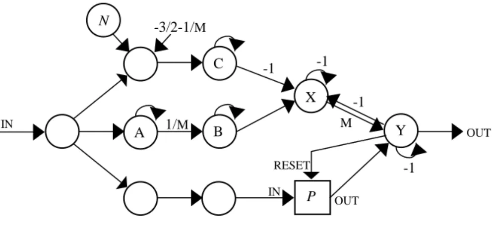
Fig. 17. Timer Constructor:
CYCLE(
N)
P. All subnets are denoted by squares.
Several timer constructs can be used sequentially. For e.g.,
CYCLE(10000)
TRY(50)
IFflag
= 1
THEN SEND X INTO C;
means that on each 10 000 cycles, it will check if an integer variable ‘flag’ has
value 1. If it is, send value X through channel C. If the variable cannot be sent in 50
cycles, abort execution.
2.9.
Non Determinism
The
CHOOSE
construct introduces non determinism in
NETDEF
. Process
CHOOSE
non
deterministically selects one of its instructions and executes it.
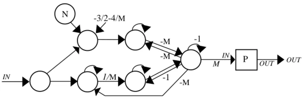
choose ::= “
CHOOSE” instruction “;”instruction { “;” instruction } “
ENDCHOOSE”.
To do so,
NETDEF
has a special input
GUESS
that returns random binary values. If
we have
N
instructions, there is the need of
K
=
log
2N
bits of information in order
to choose one of them. To do so,
CHOOSE
picks
K
(binary) values from
GUESS
, b
1,
b
2, …, bK; and use them to activate instruction number
M
= b
1b
2…bK , (in binary
notation). If
M
>
N
, then
CHOOSE
tries again.
OUT
-1
-M
M1/M
-3/2-3/M
-1
INN
P
IN OUT OUT IN OUT-M
-M
-1
-M
M1/
M-3/2-4/M
-1
INN
P
Fig. 18. Choosing between three instructions (i.e.,
CHOOSEneeds two random bits)
.All subnets are denoted by squares.
The weights between neurons b
iand neurons 01 and 10 are not presented for clarity
reasons. But the main idea is to activate one specific neuron for each binary string
obtained.
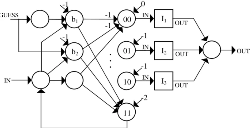
2.10. Exceptions
In high-level languages, like Eiffel
®[
Interactive 89
]
or Ada
®[USDD 83],
exceptions are unexpected events occurring during the execution of a system and
disrupting the normal flow of execution (e.g., division by zero or an operation
overflow). Some exceptions are raised by the system, others by the program itself.
The (hypothetical) neural net hardware is homogenous, there is no system
disruption other than neuron (in one of the operations or in the activation function
computation) or sinapse failure.
Despite the possibility of system failures, our concern herein will be only about
programmer raised exceptions. These exceptions adds some extra block control.
They appear as part of a
SEQ
or
PAR
block. First, an example,
meth1-failed :=
FALSE;
SEQIF
meth1-failed
THENmethod-1 -- with a ‘
RAISEexcp-1’
ELSE
method-2
; --
with a ‘
RAISEexcp-2’
job-accomplished :=
TRUE;
EXCEPTION WHENexcp-1
DOSEQ
meth1-failed:=
TRUE;
RETRY
;
ENDSEQ
;
WHENexcp-2
DO SEQjob-accomplished :=
FALSE;
TERMINATE
;
ENDSEQ;
ENDSEQ;
Suppose we have two methods to do the same work. In this sequential block, if the
first method fails, it raises an exception called ‘excp-1’ trapped by the handler part
of the block. It changes the value of the boolean variable and then execute the
block again, trying the second method. If this also fails, then the block terminates
with a no job accomplishment status.
00
b
101
10
11
b
2 IN OUT GUESS OUTI
1 IN OUTI
2 IN OUTI
3 IN0
-1
-1
-2
-1
-1
.
.
.
-1
-1
Process
RAISE
E
raises exception
E
. Each exception has an associated process (that
can be again a
SEQ
or
PAR
block), and some special block handlers. These block
handlers define what do to with the actual block:
RETRY
- reset and execute the block again,
ABORT
- reset and terminate the block,
PROPAGATE
- reset the block and raise the same exception in the upper block.
Each instruction block with an exception part, has its net architecture changed.
Fig. 19. The exception handler E of instruction block B
.Block I
Eis the instruction associated with exception E.
All subnets are denoted by squares.
Each exception has a specific neuron receiving the block process signal. With this
type of structure,
RAISE
is defined as,
PAR
E
:=1;
≡
RAISE E STOP
;
ENDPAR
;
There is a cascade effect for no handled exceptions. If a block raises an exception
E
but has no handler for it, the compiler inserts by default the following handler,
WHEN E DO PROPAGATE;
Any process sending this signal is not resumed (unless one of the upper blocks
retries its execution).
2.11. Space and Time Complexity
The proposed implementation map is able to translate any given
NETDEF
program to
an analog recurrent (rational) neural net that performs the same computations. We
wonder what is the space complexity of the implementation, i.e., how many
neurons are needed to support a given
NETDEF
program? We take a close look at
each basic process, to evaluate its contribution to the size of the final net.
The assignment inserts 3 neurones plus those that are needed to compute the
expression. The
SKIP
and
STOP
needs only one neuron. The
IF
-
THEN
-
ELSE
needs 4,
and the
WHILE
needs 5 neurons. The
SEQ
statement needs no neurons and the
PAR
of
n processes needs n+2 neurons.
SEND
needs 5 neurons and
RECEIVE
needs 4. Timers
also have constant number of neurons. All other processes have the same behaviour
about the number of neurons.
Data types and operators need a constant or linear number of neurons to the size of
the used information. All expressions can be evaluated with a linear growth in that
B
RESET To upper block PROPAGATE ABORT RETRYE
I
E IN IN IN OUT OUT OUTE
Concerning time complexity, each subnet executes its respective command with a
constant delay.
NETDEF
adds a linear time slow down to the complexity of the
corresponding program.
3.
Application
3.1.
Replicated Workers
To illustrate the use of
NETDEF
, we present an example based on the Replicated
Worker paradigm. There are several parallel algorithms in which the computing
tasks are not known in advance, but are generated dynamically as the program runs.
In these algorithms, the computing tasks cannot be initially divided among the
available processes. In order to achieve a balanced load, the tasks must be assigned
to processors in a dynamic manner as they are created during the algorithm
execution.
In the Replicated Worker standpoint, an abstract data structure, called Work Pool
(WP), is used. A WP is a collection of task descriptions, each one identifying a
specific task to be performed by any of the available workers. When a worker ends
a task, it gets a new task descriptor from the WP and performs the required
computation. During this process, the worker may produce new tasks, which are
added to the WP (for more details, see [Lester 93]).
The WP has two associated primitives,
GETWORK
and
PUTWORK
, through which the
workers may access the WP set of available tasks. A worker fetches one task using
operation
GETWORK
and may call
PUTWORK
several times during that task
processing. The worker will keep fetching tasks until it receives a special
termination task.
There is an important issue, termination. When WP ends its processing? The
obvious answer is when there is no more work to do! This is a problem because it
is a global property, it depends on WP state and of all workers. It is not enough to
see if WP is empty, since there is the possibility of an active worker still add some
new tasks to be processed. The algorithm must terminate if and only if all workers
are idle and there is no task in WP.
3.2.
The
NETDEF
program
There are three major structures in
NETDEF
implementation of Replicated Workers,
the WP, the worker and the shared structure that will ensure termination.
3.2.1. The Work Pool
The WP will be a queue with a limited number of tasks. The FIFO discipline is
good to achieve fairness in task assignation (it could be implemented with levels of
priority). This is the
NETDEF
code for the queue data structure and its associated
primitives,
INIWP
,
PUTTASK
and
GETTASK
,
CONST
endWork
= 0; -- special task termination
VAR
task : integer; --
task descriptor
wkPool :
ARRAY[100]
OFinteger;
firstTask, lastTask : integer;
FUNCTION
iniWP
ISNIL
SEQfirstTask := 1;
lastTask := 1;
ENDSEQ;
FUNCTION
putTask ( Task : integer )
ISNIL
SEQIF
mod(lastTask+1, 100) = firstTask
THEN RAISE
wkPoolFull
ELSE SEQ
lastTask := mod(lastTask+1, 100);
wkPool[lastTask] := Task;
ENDSEQ
;
EXCEPTIONWHEN
wkPoolFull
DO RETRY;
ENDSEQ;
FUNCTION
getTask (
VARTask : integer )
ISNIL
SEQIF
lastTask = firstTask
THEN RAISE
wkPoolEmpty
ELSE SEQ
Task := wkPool[firstTask] ;
firstTask := mod(firstTask+1, 100);
ENDSEQ
;
EXCEPTION
WHEN
wkPoolEmpty
DO RETRY;
ENDSEQ;
Procedures
GETTASK
and
PUTTASK
use exception handlers when the queue is empty
or full respectively. It is expected that some other worker will solve the situation. If
that does not happen, the system will deadlock. Hence, a greater queue is needed.
3.2.2. Termination
To handle termination we will use a global shared integer variable workCount.
When it is positive it keeps how many tasks are at that moment in the WP. If it is
not positive, it says that there are no tasks in the WP and there are |workCount|
workers in an idle state. So, when the variable is equal to -(number of workers), the
WP must terminate. We use the following procedure to update this value:
FUNCTION
updateCount
( isGet
: boolean
)
ISNIL
IFisGet
THENworkCount := pred(workCount)
ELSE
workCount := succ(workCount);
Since workCount is only modified inside procedure
UPDATE
C
OUNT
, it works like a
locked shared variable. This control will be done by the
GETWORK
procedure.
When trying to get a work, if it sees that the termination condition is true, it raises
an exception sending (number of workers-1) special termination tasks to the WP
and terminates itself.
FUNCTION
putWork ( Task : integer )
ISNIL
SEQupdateCount( FALSE );
putTask( Task );
ENDSEQ;
FUNCTION
getWork (
VARTask : integer )
ISNIL
SEQVAR
i :
INTEGER;
updateCount(
TRUE);
IF
workCount = -nWorkers
THEN RAISE
TerminateWP
ELSE
getTask( Task );
EXCEPTIONWHEN
TerminateWP
DO SEQi := 1;
while i < nWorkers do
putTask( endWork );
ABORT
;
ENDSEQ;
ENDSEQ;
3.2.3. The worker
The workers are instances of the same worker model. Of course, each problem
requires a specific worker model. Herein, we present its usual structure. The code
consists of a main loop that stars with a first getWork procedure call. During the
execution of that work, it may generate new tasks and subsequently call
PUT
W
ORK
several times to add these new tasks to the WP. It may also have some access to
shared data. These accesses must be handled by techniques similar to the one used
in procedure updateCount.
SEQ
-- code template for worker
VARTask : integer;
…
getwork( Task );
WHILE
Task <> endWork
DOSEQ
… --
with some putWork calls
getwork( Task );
ENDSEQ
;
ENDSEQ
;
3.2.4. Main Program
The main program will be:
NETDEFWorkPool
IS
... – variables and procedures declaration
SEQVAR
iniTask : integer;
PARworkCount := 1;
iniWP;
… --
construction of iniTask
ENDPAR;
putTask( iniTask );
PAR... – worker code repeated as many times as needed
ENDPAR;
ENDSEQ
;
ENDDEF.
4.
Conclusions
We introduced the core of a new language,
NETDEF
.
NETDEF
develops an easy way
to build neural nets performing arbitrarily complex computations. This method is
modular, where each process is mapped in an independent neural net. Modularity
brings great flexibility. For example, if a certain task is programmed and compiled,
the resulting net is a module that can be used elsewhere.
The Replicated Workers paradigm was used as an example of parallel
programming in
NETDEF
. It was shown how to make procedure calls to lock access
to shared variables in a truly synchronous parallel architecture.
The use of finite neural networks as deterministic machines to implement arbitrary
complex algorithms is now possible by the automation of compilers like
NETDEF
. If
someday, neural net hardware would be as easy to build as Von Neumann
hardware, then the
NETDEF
approach will provide a way to insert algorithms into
the massive parallel architecture of artificial neural nets. To test our program, able
to compile and simulate the dynamics of neural nets described in this paper, go to
www.di.fc.ul.pt/~jpn/netdef/netdef.htm.
5.
References
[
I
NTERACTIVE
89
]
Interactive Software Engineering Inc., Eiffel
®: the Language, TR-EI 17/RM,
1989.
[
G
RUAU
et al. 95
]
Gruau, F.; Ratajszczak, J. and Wiber, G., A Neural Compiler, Theoretical
Computer Science, [141] (1-2), 1995, 1-52.
[
L
ESTER
93
]
Lester, B. P., The Art of Parallel Programming, 1993, Prentice Hall.
[
M
C
C
ULLOCH
and
P
ITTS
43
]
McCulloch, W. and Pitts, W., A Logical Calculus of the Ideas Immanent in
Nervous Activity, Bulletin of Mathematical Biophysics, 5, 1943, 115-133.
[
M
INSKY
67
]
Minsky, M., Computation: Finite and Infinite Machines, Prentice Hall, 1967.
[
N
ETO
et al. 97
]
Neto, J. P., Siegelmann, H., Costa, J. F., Araujo, C. S., Turing Universality of
Neural Nets (revisited), Lecture Notes in Computer Science – 1333,
Springer-Verlag, 1997, 361-366.
[
S
IEGELMANN
and
S
ONTAG
95
]
Siegelmann, H. and Sontag, E., On the Computational Power of Neural Nets,
Journal of Computer and System Sciences [50] 1, Academic Press, 1995,
132-150.
[
S
IEGELMANN
96
]
Siegelmann, H., On NIL: The Software Constructor of Neural Networks,
Parallel Processing Letters, [6] 4, World Scientific Publishing Company,
[
S
IEGELMANN
99
]
Siegelmann, H., Neural Networks and Analog Computation, Beyond the
Turing Limit, Birkhauser, 1999.
[SGS-T
HOMSOM
95]
SGS-THOMSON, Occam
®2.1 Reference Manual, 1995.
[S
ONTAG
90]
Sontag, E., Mathematical Control Theory: Deterministic Finite Dimensional
Systems, Springer-Verlag, New York, 1990.
[USDD 83]
United States Department of Defence, Reference Manual for the Ada
®Programming Language, American National Standards Institute Inc., 1983.
[W
ATT
90]
Watt, D., Programming Language Concepts and Paradigms, Prentice Hall
International Series in Computer Science, 1990.
Appendix A –
NETDEF
Code for WorkPool sample
NETDEF netName(0,0) IS --NORESET
CONST
endWork = 0; -- special task termination
VAR
task : integer; --
task descriptor
wkPool : array [10] of integer;
firstTask, lastTask, sizePool, i, j : integer;
workCount, nWorkers : integer;
b : boolean;
---FUNCTION mod( x : integer; y : integer ) IS INTEGER
SEQ
WHILE x>=y DO x := x-y;
RETURN x;
ENDSEQ;
-- initialize WorkPool structure
FUNCTION iniWP IS NIL
SEQ
firstTask := 1;
lastTask := 1;
sizePool := 10;
endWork := 255;
ENDSEQ;
-- insert a Task into the WorkPool
FUNCTION putTask ( Task : integer ) IS NIL
SEQ
i := lastTask+1;
j := mod(i, sizePool);
IF j = firstTask
THEN RAISE wkPoolFull
ELSE SEQ
lastTask := mod(i, sizePool);
wkPool[lastTask] := Task;
ENDSEQ;
EXCEPTION
WHEN wkPoolFull DO RETRY;
ENDSEQ;
-- get a Task from the WorkPool
FUNCTION getTask ( var Task : integer ) IS NIL
SEQ
VAR i : integer;
IF lastTask = firstTask
THEN RAISE wkPoolEmpty
ELSE SEQ
Task := wkPool[firstTask] ;
i := firstTask+1;
firstTask := mod(i, sizePool);
ENDSEQ;
EXCEPTION
WHEN wkPoolEmpty DO RETRY;
ENDSEQ;
IF isGet THEN workCount := pred(workCount)
ELSE workCount := succ(workCount);
-- insert Work to be done
FUNCTION putWork ( Task : integer ) IS NIL
SEQ
b := false;
updateCount( b );
putTask( Task );
ENDSEQ;
-- get undone Work
FUNCTION getWork ( var Task : integer ) IS NIL
SEQ
VAR i : integer;;
b := true;
updateCount( b );
IF workCount = - nWorkers
THEN RAISE TerminateWP
ELSE getTask( Task );
EXCEPTION
WHEN TerminateWP DO
SEQ
i := 1;
WHILE i < nWorkers DO
putTask( endWork );
ABORT;
ENDSEQ;
ENDSEQ;
---SEQ -- Main Block
VAR iniTask, Task1 : integer;
PAR
workCount := 1;
nWorkers := 1;
iniWP();
ENDPAR;
putTask( iniTask );
PAR -- workers...
SEQ -- worker1
getWork( Task1 );
WHILE Task1 <> endWork DO
SEQ
--
with some putWork calls
getWork( Task1 );
ENDSEQ;
ENDSEQ; -- endWorker1
ENDPAR;
ENDSEQ;
ENDDEF.
Appendix B – Neural net structure of the previous code (679 neurons and
1438 synapses)
Mn0In(i+1) = sigma( )
Mn0Out(i+1) = sigma( + 1,0 * SEQ10Out(i) )
CONI:endWork(i+1) = sigma( - 1,0 * VI8Out(i) + 1,0 * ATR5ExpR(i) + 0,5 ) VARIMn0:task(i+1) = sigma( + 1,0 * VARIMn0:task(i) )
VARIMn0:wkPoolIn(i+1) = sigma( + 1,0 * ATR9dW(i) + 1,0 * VV17Out(i) ) VARIMn0:wkPoolOut(i+1) = sigma( + 1,0 * VARIMn0:wkPoold3In(i) + 1,0 *
VARIMn0:wkPoold7In(i) )
VARIMn0:wkPoolResl(i+1) = sigma( + 1,0 * VARIMn0:wkPool[1]6(i) + 1,0 * VARIMn0:wkPool[2]6(i) + 1,0 * VARIMn0:wkPool[3]6(i) + 1,0 * VARIMn0:wkPool[4]6(i) + 1,0 * VARIMn0:wkPool[5]6(i) + 1,0 * VARIMn0:wkPool[6]6(i) + 1,0 * VARIMn0:wkPool[7]6(i) + 1,0 * VARIMn0:wkPool[8]6(i) + 1,0 * VARIMn0:wkPool[9]6(i) + 1,0 * VARIMn0:wkPool[10]6(i) )
VARIMn0:wkPoolVal(i+1) = sigma( + 1,0 * ATR9dVal(i) )
VARIMn0:wkPooldV(i+1) = sigma( + 1,0 * VARIMn0:wkPoolIn(i) + 1,0 * VARIMn0:wkPoolVal(i) - 1,0 )
VARIMn0:wkPoolddV(i+1) = sigma( + 1,0 * VARIMn0:wkPooldV(i) ) VARIMn0:wkPoold3V(i+1) = sigma( + 1,0 * VARIMn0:wkPoolddV(i) ) VARIMn0:wkPoolId(i+1) = sigma( + 1,0 * ATR9dId(i) )
VARIMn0:wkPooldId(i+1) = sigma( + 1,0 * VARIMn0:wkPoolIn(i) + 1,0 * VARIMn0:wkPoolId(i) - 1,0 )
VARIMn0:wkPooldIn(i+1) = sigma( + 1,0 * VARIMn0:wkPoolIn(i) + 2E13 * VARIMn0:wkPoolId(i) - 1,0 )
VARIMn0:wkPoolddIn(i+1) = sigma( + 1,0 * VARIMn0:wkPooldIn(i) ) VARIMn0:wkPoold3In(i+1) = sigma( + 1,0 * VARIMn0:wkPoolddIn(i) ) VARIMn0:wkPoold4In(i+1) = sigma( + 1,0 * VARIMn0:wkPoolIn(i) + 2E13 *
VARIMn0:wkPoolValO(i) - 1,0 )
VARIMn0:wkPoold5In(i+1) = sigma( + 1,0 * VARIMn0:wkPoold4In(i) ) VARIMn0:wkPoold6In(i+1) = sigma( + 1,0 * VARIMn0:wkPoold5In(i) ) VARIMn0:wkPoold7In(i+1) = sigma( + 1,0 * VARIMn0:wkPoold6In(i) ) VARIMn0:wkPoolValO(i+1) = sigma( + 1,0 * VV17Resl(i) )
VARIMn0:wkPooldVO(i+1) = sigma( + 1,0 * VARIMn0:wkPoolIn(i) + 1,0 * VARIMn0:wkPoolValO(i) - 1,0 )
VARIMn0:wkPool[1](i+1) = sigma( + 1,0 * VARIMn0:wkPool[1](i) - 1,0 * VARIMn0:wkPool[1]2(i) + 1,0 * VARIMn0:wkPool[1]3(i) + 1,0 * VARIMn0:wkPool[2]2(i) )
VARIMn0:wkPool[1]1(i+1) = sigma( + 1,0 * VARIMn0:wkPooldId(i) - 0,5 ) VARIMn0:wkPool[1]2(i+1) = sigma( + 2E13 * VARIMn0:wkPool[1]1(i) ) VARIMn0:wkPool[1]3(i+1) = sigma( + 1,0 * VARIMn0:wkPoold3V(i) + 1,0 *
VARIMn0:wkPool[1]2(i) - 1,0 * VARIMn0:wkPool[2]2(i) - 1,0 )
VARIMn0:wkPool[1]4(i+1) = sigma( + 1,0 * VARIMn0:wkPooldVO(i) - 0,50000000000001 ) VARIMn0:wkPool[1]5(i+1) = sigma( + 2E13 * VARIMn0:wkPool[1]4(i) )
VARIMn0:wkPool[1]6(i+1) = sigma( + 1,0 * VARIMn0:wkPool[1](i) + 1,0 * VARIMn0:wkPool[1]5(i) - 1,0 * VARIMn0:wkPool[2]5(i) - 1,0 ) VARIMn0:wkPool[2](i+1) = sigma( + 1,0 * VARIMn0:wkPool[2](i) - 1,0 *
VARIMn0:wkPool[2]2(i) + 1,0 * VARIMn0:wkPool[2]3(i) + 1,0 * VARIMn0:wkPool[3]2(i) )
VARIMn0:wkPool[2]1(i+1) = sigma( + 1,0 * VARIMn0:wkPooldId(i) - 0,5000000000001 ) VARIMn0:wkPool[2]2(i+1) = sigma( + 2E13 * VARIMn0:wkPool[2]1(i) )
VARIMn0:wkPool[2]3(i+1) = sigma( + 1,0 * VARIMn0:wkPoold3V(i) + 1,0 * VARIMn0:wkPool[2]2(i) - 1,0 * VARIMn0:wkPool[3]2(i) - 1,0 )
VARIMn0:wkPool[2]4(i+1) = sigma( + 1,0 * VARIMn0:wkPooldVO(i) - 0,50000000000011 ) VARIMn0:wkPool[2]5(i+1) = sigma( + 2E13 * VARIMn0:wkPool[2]4(i) )
VARIMn0:wkPool[2]6(i+1) = sigma( + 1,0 * VARIMn0:wkPool[2](i) + 1,0 * VARIMn0:wkPool[2]5(i) - 1,0 * VARIMn0:wkPool[3]5(i) - 1,0 ) VARIMn0:wkPool[3](i+1) = sigma( + 1,0 * VARIMn0:wkPool[3](i) - 1,0 *
VARIMn0:wkPool[3]2(i) + 1,0 * VARIMn0:wkPool[3]3(i) + 1,0 * VARIMn0:wkPool[4]2(i) )
VARIMn0:wkPool[3]1(i+1) = sigma( + 1,0 * VARIMn0:wkPooldId(i) - 0,5000000000002 ) VARIMn0:wkPool[3]2(i+1) = sigma( + 2E13 * VARIMn0:wkPool[3]1(i) )
VARIMn0:wkPool[3]3(i+1) = sigma( + 1,0 * VARIMn0:wkPoold3V(i) + 1,0 * VARIMn0:wkPool[3]2(i) - 1,0 * VARIMn0:wkPool[4]2(i) - 1,0 )
VARIMn0:wkPool[3]4(i+1) = sigma( + 1,0 * VARIMn0:wkPooldVO(i) - 0,50000000000021 ) VARIMn0:wkPool[3]5(i+1) = sigma( + 2E13 * VARIMn0:wkPool[3]4(i) )
VARIMn0:wkPool[3]6(i+1) = sigma( + 1,0 * VARIMn0:wkPool[3](i) + 1,0 * VARIMn0:wkPool[3]5(i) - 1,0 * VARIMn0:wkPool[4]5(i) - 1,0 ) VARIMn0:wkPool[4](i+1) = sigma( + 1,0 * VARIMn0:wkPool[4](i) - 1,0 *
VARIMn0:wkPool[4]3(i+1) = sigma( + 1,0 * VARIMn0:wkPoold3V(i) + 1,0 * VARIMn0:wkPool[4]2(i) - 1,0 * VARIMn0:wkPool[5]2(i) - 1,0 )
VARIMn0:wkPool[4]4(i+1) = sigma( + 1,0 * VARIMn0:wkPooldVO(i) - 0,50000000000031 ) VARIMn0:wkPool[4]5(i+1) = sigma( + 2E13 * VARIMn0:wkPool[4]4(i) )
VARIMn0:wkPool[4]6(i+1) = sigma( + 1,0 * VARIMn0:wkPool[4](i) + 1,0 * VARIMn0:wkPool[4]5(i) - 1,0 * VARIMn0:wkPool[5]5(i) - 1,0 ) VARIMn0:wkPool[5](i+1) = sigma( + 1,0 * VARIMn0:wkPool[5](i) - 1,0 *
VARIMn0:wkPool[5]2(i) + 1,0 * VARIMn0:wkPool[5]3(i) + 1,0 * VARIMn0:wkPool[6]2(i) )
VARIMn0:wkPool[5]1(i+1) = sigma( + 1,0 * VARIMn0:wkPooldId(i) - 0,5000000000004 ) VARIMn0:wkPool[5]2(i+1) = sigma( + 2E13 * VARIMn0:wkPool[5]1(i) )
VARIMn0:wkPool[5]3(i+1) = sigma( + 1,0 * VARIMn0:wkPoold3V(i) + 1,0 * VARIMn0:wkPool[5]2(i) - 1,0 * VARIMn0:wkPool[6]2(i) - 1,0 )
VARIMn0:wkPool[5]4(i+1) = sigma( + 1,0 * VARIMn0:wkPooldVO(i) - 0,50000000000041 ) VARIMn0:wkPool[5]5(i+1) = sigma( + 2E13 * VARIMn0:wkPool[5]4(i) )
VARIMn0:wkPool[5]6(i+1) = sigma( + 1,0 * VARIMn0:wkPool[5](i) + 1,0 * VARIMn0:wkPool[5]5(i) - 1,0 * VARIMn0:wkPool[6]5(i) - 1,0 ) VARIMn0:wkPool[6](i+1) = sigma( + 1,0 * VARIMn0:wkPool[6](i) - 1,0 *
VARIMn0:wkPool[6]2(i) + 1,0 * VARIMn0:wkPool[6]3(i) + 1,0 * VARIMn0:wkPool[7]2(i) )
VARIMn0:wkPool[6]1(i+1) = sigma( + 1,0 * VARIMn0:wkPooldId(i) - 0,5000000000005 ) VARIMn0:wkPool[6]2(i+1) = sigma( + 2E13 * VARIMn0:wkPool[6]1(i) )
VARIMn0:wkPool[6]3(i+1) = sigma( + 1,0 * VARIMn0:wkPoold3V(i) + 1,0 * VARIMn0:wkPool[6]2(i) - 1,0 * VARIMn0:wkPool[7]2(i) - 1,0 )
VARIMn0:wkPool[6]4(i+1) = sigma( + 1,0 * VARIMn0:wkPooldVO(i) - 0,50000000000051 ) VARIMn0:wkPool[6]5(i+1) = sigma( + 2E13 * VARIMn0:wkPool[6]4(i) )
VARIMn0:wkPool[6]6(i+1) = sigma( + 1,0 * VARIMn0:wkPool[6](i) + 1,0 * VARIMn0:wkPool[6]5(i) - 1,0 * VARIMn0:wkPool[7]5(i) - 1,0 ) VARIMn0:wkPool[7](i+1) = sigma( + 1,0 * VARIMn0:wkPool[7](i) - 1,0 *
VARIMn0:wkPool[7]2(i) + 1,0 * VARIMn0:wkPool[7]3(i) + 1,0 * VARIMn0:wkPool[8]2(i) )
VARIMn0:wkPool[7]1(i+1) = sigma( + 1,0 * VARIMn0:wkPooldId(i) - 0,5000000000006 ) VARIMn0:wkPool[7]2(i+1) = sigma( + 2E13 * VARIMn0:wkPool[7]1(i) )
VARIMn0:wkPool[7]3(i+1) = sigma( + 1,0 * VARIMn0:wkPoold3V(i) + 1,0 * VARIMn0:wkPool[7]2(i) - 1,0 * VARIMn0:wkPool[8]2(i) - 1,0 )
VARIMn0:wkPool[7]4(i+1) = sigma( + 1,0 * VARIMn0:wkPooldVO(i) - 0,50000000000061 ) VARIMn0:wkPool[7]5(i+1) = sigma( + 2E13 * VARIMn0:wkPool[7]4(i) )
VARIMn0:wkPool[7]6(i+1) = sigma( + 1,0 * VARIMn0:wkPool[7](i) + 1,0 * VARIMn0:wkPool[7]5(i) - 1,0 * VARIMn0:wkPool[8]5(i) - 1,0 ) VARIMn0:wkPool[8](i+1) = sigma( + 1,0 * VARIMn0:wkPool[8](i) - 1,0 *
VARIMn0:wkPool[8]2(i) + 1,0 * VARIMn0:wkPool[8]3(i) + 1,0 * VARIMn0:wkPool[9]2(i) )
VARIMn0:wkPool[8]1(i+1) = sigma( + 1,0 * VARIMn0:wkPooldId(i) - 0,5000000000007 ) VARIMn0:wkPool[8]2(i+1) = sigma( + 2E13 * VARIMn0:wkPool[8]1(i) )
VARIMn0:wkPool[8]3(i+1) = sigma( + 1,0 * VARIMn0:wkPoold3V(i) + 1,0 * VARIMn0:wkPool[8]2(i) - 1,0 * VARIMn0:wkPool[9]2(i) - 1,0 )
VARIMn0:wkPool[8]4(i+1) = sigma( + 1,0 * VARIMn0:wkPooldVO(i) - 0,50000000000071 ) VARIMn0:wkPool[8]5(i+1) = sigma( + 2E13 * VARIMn0:wkPool[8]4(i) )
VARIMn0:wkPool[8]6(i+1) = sigma( + 1,0 * VARIMn0:wkPool[8](i) + 1,0 * VARIMn0:wkPool[8]5(i) - 1,0 * VARIMn0:wkPool[9]5(i) - 1,0 ) VARIMn0:wkPool[9](i+1) = sigma( + 1,0 * VARIMn0:wkPool[9](i) - 1,0 *
VARIMn0:wkPool[9]2(i) + 1,0 * VARIMn0:wkPool[9]3(i) + 1,0 * VARIMn0:wkPool[10]2(i) )
VARIMn0:wkPool[9]1(i+1) = sigma( + 1,0 * VARIMn0:wkPooldId(i) - 0,5000000000008 ) VARIMn0:wkPool[9]2(i+1) = sigma( + 2E13 * VARIMn0:wkPool[9]1(i) )
VARIMn0:wkPool[9]3(i+1) = sigma( + 1,0 * VARIMn0:wkPoold3V(i) + 1,0 * VARIMn0:wkPool[9]2(i) - 1,0 * VARIMn0:wkPool[10]2(i) - 1,0 )
VARIMn0:wkPool[9]4(i+1) = sigma( + 1,0 * VARIMn0:wkPooldVO(i) - 0,50000000000081 ) VARIMn0:wkPool[9]5(i+1) = sigma( + 2E13 * VARIMn0:wkPool[9]4(i) )
VARIMn0:wkPool[9]6(i+1) = sigma( + 1,0 * VARIMn0:wkPool[9](i) + 1,0 * VARIMn0:wkPool[9]5(i) - 1,0 * VARIMn0:wkPool[10]5(i) - 1,0 ) VARIMn0:wkPool[10](i+1) = sigma( + 1,0 * VARIMn0:wkPool[10](i) - 1,0 *
VARIMn0:wkPool[10]2(i) + 1,0 * VARIMn0:wkPool[10]3(i) )
VARIMn0:wkPool[10]1(i+1) = sigma( + 1,0 * VARIMn0:wkPooldId(i) - 0,5000000000009 ) VARIMn0:wkPool[10]2(i+1) = sigma( + 2E13 * VARIMn0:wkPool[10]1(i) )
VARIMn0:wkPool[10]3(i+1) = sigma( + 1,0 * VARIMn0:wkPoold3V(i) + 1,0 * VARIMn0:wkPool[10]2(i) - 1,0 )
VARIMn0:wkPool[10]4(i+1) = sigma( + 1,0 * VARIMn0:wkPooldVO(i) - 0,50000000000091 ) VARIMn0:wkPool[10]5(i+1) = sigma( + 2E13 * VARIMn0:wkPool[10]4(i) )
VARIMn0:wkPool[10]6(i+1) = sigma( + 1,0 * VARIMn0:wkPool[10](i) + 1,0 * VARIMn0:wkPool[10]5(i) - 1,0 )
VARIMn0:j(i+1) = sigma( + 1,0 * VARIMn0:j(i) - 1,0 * CALL1Out(i) + 1,0 * ATR7ExpR(i) )
VARIMn0:i(i+1) = sigma( + 1,0 * VARIMn0:i(i) - 1,0 * SUM1Out(i) + 1,0 * ATR6ExpR(i) )
VARIMn0:sizePool(i+1) = sigma( + 1,0 * VARIMn0:sizePool(i) - 1,0 * VI7Out(i) + 1,0 * ATR4ExpR(i) )
VARIMn0:lastTask(i+1) = sigma( + 1,0 * VARIMn0:lastTask(i) - 1,0 * VI6Out(i) + 1,0 * ATR3ExpR(i) - 1,0 * CALL2Out(i) + 1,0 * ATR8ExpR(i) )
VARIMn0:firstTask(i+1) = sigma( + 1,0 * VARIMn0:firstTask(i) - 1,0 * VI5Out(i) + 1,0 * ATR2ExpR(i) - 1,0 * CALL3Out(i) + 1,0 * ATR12ExpR(i) )
VARIMn0:nWorkers(i+1) = sigma( + 1,0 * VARIMn0:nWorkers(i) - 1,0 * VI32Out(i) + 1,0 * ATR19ExpR(i) )
VARIMn0:workCount(i+1) = sigma( + 1,0 * VARIMn0:workCount(i) - 1,0 * PRE1Out(i) + 1,0 * ATR13ExpR(i) - 1,0 * SUC1Out(i) + 1,0 * ATR14ExpR(i) - 1,0 * VI31Out(i) + 1,0 * ATR18ExpR(i) )
VARBMn0:b(i+1) = sigma( + 1,0 * VARBMn0:b(i) + 1,0 * ATR15ExpR(i) - 1,0 * VB25Out(i) + 1,0 * ATR16ExpR(i) )
FI:modIn(i+1) = sigma( + 1,0 * CALL1Bgn(i) + 1,0 * CALL2Bgn(i) + 1,0 * CALL3Bgn(i) )
FI:modOut(i+1) = sigma( + 1,0 * FI:modddOut(i) ) FI:modResl(i+1) = sigma( + 1,0 * FI:modddRes(i) ) FI:moddOut(i+1) = sigma( + 1,0 * SEQ1Out(i) ) FI:modddOut(i+1) = sigma( + 1,0 * FI:moddOut(i) ) FI:moddRes(i+1) = sigma( + 1,0 * SEQ1Resl(i) ) FI:modddRes(i+1) = sigma( + 1,0 * FI:moddRes(i) )
VARILFI:mod:x(i+1) = sigma( - 1,0 * FI:modddOut(i) + 1,0 * VARILFI:mod:x(i) + 1,0 * FI:modArg1(i) - 1,0 * SUB1Out(i) + 1,0 * ATR1ExpR(i) )
FI:modArg1(i+1) = sigma( + 1,0 * CALL1dVl1(i) + 1,0 * CALL2dVl1(i) + 1,0 * CALL3dVl1(i) )
VARILFI:mod:y(i+1) = sigma( - 1,0 * FI:modddOut(i) + 1,0 * VARILFI:mod:y(i) + 1,0 * FI:modArg2(i) )
FI:modArg2(i+1) = sigma( + 1,0 * CALL1dVl2(i) + 1,0 * CALL2dVl2(i) + 1,0 * CALL3dVl2(i) )
FI:mod0(i+1) = sigma( + 1,0 * Mn0In(i) + 1,0 * FI:mod3d(i) ) FI:mod0d(i+1) = sigma( + 1,0 * FI:mod0(i) )
SEQ1In(i+1) = sigma( + 1,0 * FI:modIn(i) ) SEQ1Out(i+1) = sigma( + 1,0 * SEQ1dAbr(i) ) SEQ1Reset(i+1) = sigma( + 1,0 * SEQ1Abort(i) ) SEQ1Abort(i+1) = sigma( + 1,0 * RET1In(i) ) SEQ1Resl(i+1) = sigma( + 1,0 * RET1ddRs(i) ) SEQ1dAbr(i+1) = sigma( + 1,0 * SEQ1Abort(i) )
WHL1In(i+1) = sigma( + 1,0 * SEQ1In(i) - 1,0 * SEQ1Reset(i) + 1,0 * ATR1Out(i) ) WHL1ExpR(i+1) = sigma( 1,0 * SEQ1Reset(i) + 1,0 * GE1Out(i) + 1,0 * GE1Resl(i)
-1,0 )
WHL1Out(i+1) = sigma( - 1,0 * SEQ1Reset(i) + 1,0 * GE1Out(i) - 1,0 * GE1Resl(i) ) VV1In(i+1) = sigma( - 1,0 * SEQ1Reset(i) + 1,0 * GE1In(i) )
VV1Out(i+1) = sigma( - 1,0 * SEQ1Reset(i) + 1,0 * VV1In(i) )
VV1Resl(i+1) = sigma( + 1,0 * VARILFI:mod:x(i) - 1,0 * SEQ1Reset(i) + 1,0 * VV1In(i) - 1,0 )
VV2In(i+1) = sigma( - 1,0 * SEQ1Reset(i) + 1,0 * GE1In(i) ) VV2Out(i+1) = sigma( - 1,0 * SEQ1Reset(i) + 1,0 * VV2In(i) )
VV2Resl(i+1) = sigma( + 1,0 * VARILFI:mod:y(i) - 1,0 * SEQ1Reset(i) + 1,0 * VV2In(i) - 1,0 )
GE1In(i+1) = sigma( - 1,0 * SEQ1Reset(i) + 1,0 * WHL1In(i) ) GE1Out(i+1) = sigma( - 1,0 * SEQ1Reset(i) + 1,0 * GE1d3Wt(i) )
GE1Resl(i+1) = sigma( - 1,0 * SEQ1Reset(i) - 1,0 * GE1ddRs(i) + 1,0 * GE1d3Wt(i) ) GE1dRs(i+1) = sigma( - 1,0 * GE1dLf(i) + 1,0 * GE1dRg(i) )
GE1ddRs(i+1) = sigma( + 2E13 * GE1dRs(i) ) GE1ddWt(i+1) = sigma( + 1,0 * GE1dWt(i) ) GE1d3Wt(i+1) = sigma( + 1,0 * GE1ddWt(i) )
GE1wait(i+1) = sigma( - 1,0 * SEQ1Reset(i) - 1,0 * GE1wait(i) + 1,0 * GE1wLf(i) + 1,0 * GE1wRg(i) - 1,0 )
GE1dWt(i+1) = sigma( - 1,0 * SEQ1Reset(i) + 1,0 * GE1wait(i) )
GE1vLf(i+1) = sigma( - 1,0 * SEQ1Reset(i) + 1,0 * VV1Resl(i) - 1,0 * GE1wait(i) + 1,0 * GE1vLf(i) )
GE1wLf(i+1) = sigma( - 1,0 * SEQ1Reset(i) + 1,0 * VV1Out(i) - 1,0 * GE1wait(i) + 1,0 * GE1wLf(i) )
GE1dLf(i+1) = sigma( 1,0 * SEQ1Reset(i) + 1,0 * GE1wait(i) + 1,0 * GE1vLf(i) -1,0 )
GE1vRg(i+1) = sigma( - 1,0 * SEQ1Reset(i) + 1,0 * VV2Resl(i) - 1,0 * GE1wait(i) + 1,0 * GE1vRg(i) )
GE1wRg(i+1) = sigma( - 1,0 * SEQ1Reset(i) + 1,0 * VV2Out(i) - 1,0 * GE1wait(i) + 1,0 * GE1wRg(i) )
GE1dRg(i+1) = sigma( 1,0 * SEQ1Reset(i) + 1,0 * GE1wait(i) + 1,0 * GE1vRg(i) -1,0 )
VV3In(i+1) = sigma( - 1,0 * SEQ1Reset(i) + 1,0 * SUB1In(i) ) VV3Out(i+1) = sigma( - 1,0 * SEQ1Reset(i) + 1,0 * VV3In(i) )
VV3Resl(i+1) = sigma( + 1,0 * VARILFI:mod:x(i) - 1,0 * SEQ1Reset(i) + 1,0 * VV3In(i) - 1,0 )
SUB1In(i+1) = sigma( - 1,0 * SEQ1Reset(i) + 1,0 * ATR1In(i) ) SUB1Out(i+1) = sigma( - 1,0 * SEQ1Reset(i) + 1,0 * SUB1dWt(i) )
SUB1Resl(i+1) = sigma( 1,0 * SEQ1Reset(i) + 1,0 * SUB1dWt(i) + 1,0 * SUB1dLf(i) -1,0 * SUB1dRg(i) - 0,5 )
SUB1wait(i+1) = sigma( - 1,0 * SEQ1Reset(i) - 1,0 * SUB1wait(i) + 1,0 * SUB1wLf(i) + 1,0 * SUB1wRg(i) - 1,0 )
SUB1dWt(i+1) = sigma( - 1,0 * SEQ1Reset(i) + 1,0 * SUB1wait(i) )
SUB1vLf(i+1) = sigma( - 1,0 * SEQ1Reset(i) + 1,0 * VV3Resl(i) - 1,0 * SUB1wait(i) + 1,0 * SUB1vLf(i) )
SUB1wLf(i+1) = sigma( - 1,0 * SEQ1Reset(i) + 1,0 * VV3Out(i) - 1,0 * SUB1wait(i) + 1,0 * SUB1wLf(i) )
SUB1dLf(i+1) = sigma( 1,0 * SEQ1Reset(i) + 1,0 * SUB1wait(i) + 1,0 * SUB1vLf(i) -1,0 )
SUB1vRg(i+1) = sigma( - 1,0 * SEQ1Reset(i) + 1,0 * VV4Resl(i) - 1,0 * SUB1wait(i) + 1,0 * SUB1vRg(i) )
SUB1wRg(i+1) = sigma( - 1,0 * SEQ1Reset(i) + 1,0 * VV4Out(i) - 1,0 * SUB1wait(i) + 1,0 * SUB1wRg(i) )
SUB1dRg(i+1) = sigma( 1,0 * SEQ1Reset(i) + 1,0 * SUB1wait(i) + 1,0 * SUB1vRg(i) -1,0 )
ATR1In(i+1) = sigma( - 1,0 * SEQ1Reset(i) + 1,0 * WHL1ExpR(i) )
ATR1ExpR(i+1) = sigma( - 1,0 * SEQ1Reset(i) + 1,0 * SUB1Out(i) + 1,0 * SUB1Resl(i) - 1,0 )
ATR1Out(i+1) = sigma( - 1,0 * SEQ1Reset(i) + 1,0 * SUB1Out(i) ) RET1In(i+1) = sigma( - 1,0 * SEQ1Reset(i) + 1,0 * WHL1Out(i) )
RET1dRs(i+1) = sigma( + 1,0 * VARILFI:mod:x(i) - 1,0 * SEQ1Reset(i) + 1,0 * RET1In(i) - 1,0 )
RET1ddRs(i+1) = sigma( - 1,0 * SEQ1Reset(i) + 1,0 * RET1dRs(i) ) F_:iniWPIn(i+1) = sigma( + 1,0 * CALL9Bgn(i) )
F_:iniWPOut(i+1) = sigma( + 1,0 * F_:iniWPddOut(i) ) F_:iniWPdOut(i+1) = sigma( + 1,0 * SEQ2Out(i) ) F_:iniWPddOut(i+1) = sigma( + 1,0 * F_:iniWPdOut(i) )
F_:iniWP0(i+1) = sigma( + 1,0 * Mn0In(i) + 1,0 * F_:iniWP1d(i) ) F_:iniWP0d(i+1) = sigma( + 1,0 * F_:iniWP0(i) )
SEQ2In(i+1) = sigma( + 1,0 * F_:iniWPIn(i) ) SEQ2Out(i+1) = sigma( + 1,0 * ATR5Out(i) ) VI5In(i+1) = sigma( + 1,0 * ATR2In(i) ) VI5Out(i+1) = sigma( + 1,0 * VI5In(i) )
VI5Resl(i+1) = sigma( + 1,0 * VI5In(i) - 0,4999999999999 ) ATR2In(i+1) = sigma( + 1,0 * SEQ2In(i) )
ATR2ExpR(i+1) = sigma( + 1,0 * VI5Out(i) + 1,0 * VI5Resl(i) - 1,0 ) ATR2Out(i+1) = sigma( + 1,0 * VI5Out(i) )
VI6In(i+1) = sigma( + 1,0 * ATR3In(i) ) VI6Out(i+1) = sigma( + 1,0 * VI6In(i) )
VI6Resl(i+1) = sigma( + 1,0 * VI6In(i) - 0,4999999999999 ) ATR3In(i+1) = sigma( + 1,0 * ATR2Out(i) )
ATR3ExpR(i+1) = sigma( + 1,0 * VI6Out(i) + 1,0 * VI6Resl(i) - 1,0 ) ATR3Out(i+1) = sigma( + 1,0 * VI6Out(i) )
VI7In(i+1) = sigma( + 1,0 * ATR4In(i) ) VI7Out(i+1) = sigma( + 1,0 * VI7In(i) )
VI7Resl(i+1) = sigma( + 1,0 * VI7In(i) - 0,499999999999 ) ATR4In(i+1) = sigma( + 1,0 * ATR3Out(i) )
ATR4ExpR(i+1) = sigma( + 1,0 * VI7Out(i) + 1,0 * VI7Resl(i) - 1,0 ) ATR4Out(i+1) = sigma( + 1,0 * VI7Out(i) )
VI8In(i+1) = sigma( + 1,0 * ATR5In(i) ) VI8Out(i+1) = sigma( + 1,0 * VI8In(i) )
VI8Resl(i+1) = sigma( + 1,0 * VI8In(i) - 0,4999999999745 ) ATR5In(i+1) = sigma( + 1,0 * ATR4Out(i) )
ATR5ExpR(i+1) = sigma( + 1,0 * VI8Out(i) + 1,0 * VI8Resl(i) - 1,0 ) ATR5Out(i+1) = sigma( + 1,0 * VI8Out(i) )
F_:putTaskIn(i+1) = sigma( + 1,0 * CALL5Bgn(i) + 1,0 * CALL8Bgn(i) + 1,0 * CALL10Bgn(i) )
F_:putTaskOut(i+1) = sigma( + 1,0 * F_:putTaskddOut(i) ) F_:putTaskdOut(i+1) = sigma( + 1,0 * SEQ3Out(i) )
F_:putTaskddOut(i+1) = sigma( + 1,0 * F_:putTaskdOut(i) )
VARILF_:putTask:Task(i+1) = sigma( - 1,0 * F_:putTaskddOut(i) + 1,0 * VARILF_:putTask:Task(i) + 1,0 * F_:putTaskArg1(i) )
F_:putTaskArg1(i+1) = sigma( + 1,0 * CALL5dVl1(i) + 1,0 * CALL8dVl1(i) + 1,0 * CALL10dVl1(i) )
F_:putTask0(i+1) = sigma( + 1,0 * Mn0In(i) + 1,0 * F_:putTask3d(i) ) F_:putTask0d(i+1) = sigma( + 1,0 * F_:putTask0(i) )
SEQ3In(i+1) = sigma( + 1,0 * F_:putTaskIn(i) + 1,0 * SEQ3dRet(i) ) SEQ3Out(i+1) = sigma( + 1,0 * IF1Out(i) )
SEQ3Reset(i+1) = sigma( + 1,0 * SEQ3Retry(i) ) SEQ3Retry(i+1) = sigma( + 1,0 * RTRY1In(i) ) SEQ3dRet(i+1) = sigma( + 1,0 * SEQ3Retry(i) )
VV9In(i+1) = sigma( - 1,0 * SEQ3Reset(i) + 1,0 * SUM1In(i) ) VV9Out(i+1) = sigma( - 1,0 * SEQ3Reset(i) + 1,0 * VV9In(i) )