A Tutorial on Parallel and Concurrent Programming in Haskell

(1)

A Tutorial on Parallel and Concurrent

Programming in Haskell

Simon Peyton Jones and Satnam Singh Microsoft Research Cambridge simonpj@microsoft.com satnams@microsoft.com

Abstract. This practical tutorial introduces the features available in

Haskell for writing parallel and concurrent programs. We first describe how to write semi-explicit parallel programs by using annotations to ex-press opportunities for parallelism and to help control the granularity of parallelism for effective execution on modern operating systems and pro-cessors. We then describe the mechanisms provided by Haskell for writing explicitly parallel programs with a focus on the use of software transac-tional memory to help share information between threads. Finally, we show how nested data parallelism can be used to write deterministically parallel programs which allows programmers to use rich data types in data parallel programs which are automatically transformed into flat data parallel versions for efficient execution on multi-core processors.

1 Introduction

The introduction of multi-core processors has renewed interest in parallel func-tional programming and there are now several interesting projects that explore the advantages of a functional language for writing parallel code or implicitly par-alellizing code written in a pure functional language. These lecture notes present a variety of techniques for writing concurrent parallel programs which include existing techniques based on semi-implicit parallelism and explicit thread-based parallelism as well as more recent developments in the areas of software trans-actional memory and nested data parallelism.

We also use the termsparalleland concurrentwith quite specific meanings. A parallel program is one which is written for performance reasons to exploit the potential of a real parallel computing resource like a multi-core processor. For a parallel program we have the expectation of some genuinely simultaneous execution. Concurrency is a software structuring technique that allows us to model computations as hypothetical independent activities (e.g. with their own program counters) that can communicate and synchronize.

(2)

2 Applications of concurrency and parallelism

Writing concurrent and parallel programs is more challenging than the already difficult problem of writing sequential programs. However, there are some com-pelling reasons for writing concurrent and parallel programs:

Performance. We need to write parallel programs to achieve improving per-formance from each new generation of multi-core processors.

Hiding latency. Even on single-core processors we can exploit concurrent pro-grams to hide the latency of slow I/O operations to disks and network de-vices.

Software structuring. Certain kinds of problems can be conveniently repre-sented as multiple communicating threads which help to structure code in a more modular manner e.g. by modeling user interface components as sepa-rate threads.

Real world concurrency. In distributed and real-time systems we have to model and react to events in the real world e.g. handling multiple server requests in parallel.

All new mainstream microprocessors have two or more cores and relatively soon we can expect to see tens or hundreds of cores. We can not expect the performance of each individual core to improve much further. The only way to achieve increasing performance from each new generation of chips is by dividing the work of a program across multiple processing cores. One way to divide an ap-plication over multiple processing cores is to somehow automatically parallelize the sequential code and this is an active area of research. Another approach is for the user to write a semi-explicit or explicitly parallel program which is then scheduled onto multiple cores by the operating systems and this is the approach we describe in these lectures.

3 Compiling Parallel Haskell Programs

To reproduce the results in this paper you will need to use a version of the GHC Haskell compilerlaterthan 6.10.1 (which at the time of printing requires building the GHC compiler from the HEAD branch of the source code repository). To compile a parallel Haskell program you need to specify the-threadedextra flag. For example, to compile the parallel program contained in the file Wombat.hs issue the command:

ghc --make -threaded Wombat.hs

To execute the program you need to specify how many real threads are available to execute the logical threads in a Haskell program. This is done by specifying an argument to Haskell’s run-time system at invocation time. For example, to use three real threads to execute theWombatprogram issue the command: Wombat +RTS -N3

(3)

4 Semi-Explicit Parallelism

A pure Haskell program may appear to have abundant opportunities for auto-matic parallelization. Given the lack of side effects it may seem that we can productively evaluate every sub-expression of a Haskell program in parallel. In practice this does not work out well because it creates far too many small items of work which can not be efficiently scheduled and parallelism is limited by fundamental data dependencies in the source program.

Haskell provides a mechanism to allow the user to control the granularity of parallelism by indicating what computations may be usefully carried out in parallel. This is done by using functions from the Control.Parallel module. The interface forControl.Parallelis shown below:

1 par :: a−>b−>b 2 pseq :: a−>b−>b

The functionparindicates to the Haskell run-time system that it may be benefi-cial to evaluate the first argument in parallel with the second argument. Thepar function returns as its result the value of the second argument. One can always eliminate par from a program by using the following identity without altering the semantics of the program:

1 par a b = b

The Haskell run-time system does not necessarily create a thread to compute the value of the expressiona. Instead, the run-time system creates asparkwhich has the potential to be executed on a different thread from the parent thread. A sparked computation expresses the possibility of performing some speculative evaluation. Since a thread is not necessarily created to compute the value of a this approach has some similarities with the notion of alazy future[1].

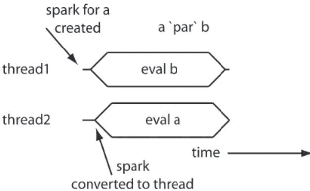
Sometimes it is convenient to write a function with two arguments as an infix function and this is done in Haskell by writing quotes around the function: 1 a ‘par‘ b

An example of this expression executing in parallel is shown in Figure1. We call such programs semi-explicitly parallel because the programmer has provided a hint about the appropriate level of granularity for parallel operations and the system implicitly creates threads to implement the concurrency. The user does not need to explicitly create any threads or write any code for inter-thread communication or synchronization.

To illustrate the use ofparwe present a program that performs two compute intensive functions in parallel. The first compute intensive function we use is the notorious Fibonacci function:

1fib ::Int−>Int 2fib 0 = 0 3fib 1 = 1

4fib n = fib (n−1) + fib (n−2)

(4)

thread1

eval a a `par` b

eval b

thread2

spark for a created

spark converted to thread

time

Fig. 1.Semi-explicit execution ofain parallel with the main threadb

1mkList ::Int−>[Int] 2mkList n = [1..n−1] 3

4relprime ::Int−>Int−>Bool 5relprime x y =gcdx y == 1 6

7euler ::Int −>Int

8euler n =length(filter(relprime n) (mkList n)) 9

10sumEuler ::Int−>Int

11sumEuler =sum. (mapeuler) . mkList

The function that we wish to parallelize adds the results of calling fib and sumEuler:

1sumFibEuler ::Int−>Int−>Int 2sumFibEuler a b = fib a + sumEuler b

As a first attempt we can try to use parthe speculatively spark off the compu-tation offibwhile the parent thread works onsumEuler:

1parSumFibEuler ::Int−>Int−>Int 2parSumFibEuler a b

3 = f ‘par‘ (f + e)

4 where

5 f = fib a 6 e = sumEuler b

To help measure how long a particular computation is taking we use theSytem.Time module and define a function that returns the difference between two time sam-ples as a number of seconds:

(5)

3 =fromInteger(psecs2−psecs1) / 1e12 +fromInteger(secs2−secs1)

The main program calls thesumFibEulerfunction with suitably large arguments and reports the value

1r1 ::Int

2r1 = sumFibEuler 38 5300 3

4main ::IO() 5main

6 =dot0<−getClockTime 7 pseq r1 (return()) 8 t1<−getClockTime

9 putStrLn(”sum: ” ++showr1)

10 putStrLn(”time: ” ++show(secDiff t0 t1) ++ ” seconds”)

The calculations fib 38and sumEuler 5300have been chosen to have roughly the same execution time.

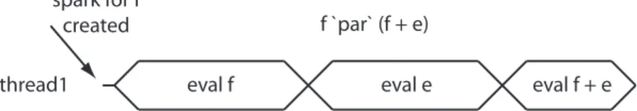
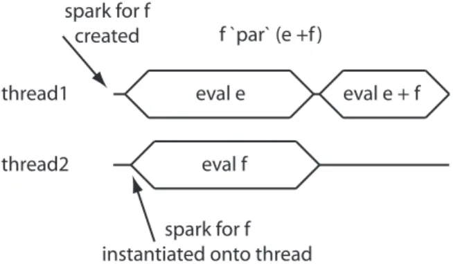
If we were to execute this code using just one thread we would observe the sequence of evaluations shown in Figure 2. Although a spark is created for the evaluation of f there is no other thread available to instantiate this spark so the program first computes f (assuming the + evaluates its left argument first) and then computes e and finally the addition is performed. Making an assumption about the evaluation order of the arguments of + is unsafe and another valid execution trace for this program would involve first evaluating e and then evaluatingf.

thread1 eval e eval f + e f `par` (f + e)

eval f spark for f

created

Fig. 2.Executingf ‘par‘ (e + f)on a single thread

The compiled program can now be run on a multi-core computer and we can see how it performs when it uses one and then two real operating system threads:

$ ParSumFibEuler +RTS -N1 sum: 47625790

time: 9.274 seconds

$ ParSumFibEuler +RTS -N2 sum: 47625790

(6)

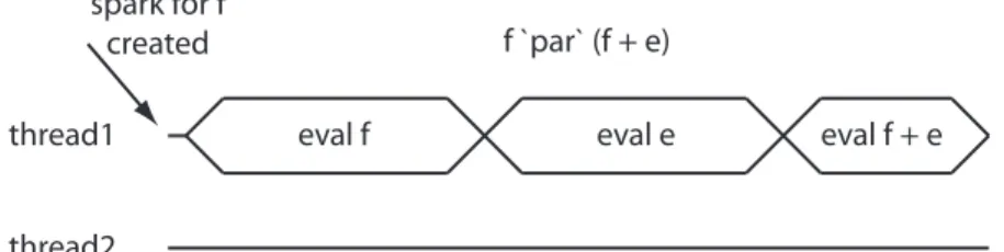
The output above shows that the version run with two cores did not perform any better than the sequential version. Why is this? The problem lies in line 3 of the parSumFibEuler function. Although the work of computing fib 38 is sparked off for speculative evaluation the parent thread also starts off by trying to compute fib 38 because this particular implementation of the program used a version of +that evaluates its left and side before it evaluates its right hand side. This causes the main thread to demand the evaluation of fib 38 so the spark never gets instantiated onto a thread. After the main thread evaluatesfib 38 it goes onto evaluatesumEuler 5300 which results in a performance which is equivalent to the sequential program. A sample execution trace for this version of the program is shown in Figure 3. We can obtain further information about

thread1 eval e eval f + e f `par` (f + e)

eval f spark for f

created

thread2

Fig. 3.A spark that does not get instantiated onto a thread

what happened by asking the run-time system to produce a log which contains information about how many sparks were created and then actually evaluated as well as information about how much work was performed by each thread. The -sflag by itself will write out such information to standard output or it can be followed by the name of a log file.

$ ParSumFibEuler +RTS -N2 -s .\ParSumFibEuler +RTS -N2 -s sum: 47625790

time: 9.223 seconds ...

SPARKS: 1 (0 converted, 0 pruned)

INIT time 0.00s ( 0.01s elapsed) MUT time 8.75s ( 8.79s elapsed) GC time 0.42s ( 0.43s elapsed) EXIT time 0.00s ( 0.00s elapsed) Total time 9.17s ( 9.23s elapsed) ...

(7)

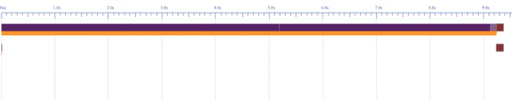
which shows one thread busy all the time but the second thread performs no work at all. Purple (or black) indicates that a thread is running and orange (or gray) indicates garbage collection.

Fig. 4.A ThreadScope trace showing lack of parallelism

A tempting fix is to reverse the order of the arguments to+: 1parSumFibEuler ::Int−>Int−>Int

2parSumFibEuler a b 3 = f ‘par‘ (e + f)

4 where

Here we are sparking off the computation offibfor speculative evaluation with respect to the parent thread. The parent thread starts off by computingsumEuler and hopefully the run-time will convert the spark for computingfiband execute it on a thread located on a different core in parallel with the parent thread. This does give a respectable speedup:

$ ParFibSumEuler2 +RTS -N1 sum: 47625790

time: 9.158 seconds

$ ParFibSumEuler2 +RTS -N2 sum: 47625790

time: 5.236 seconds

A sample execution trace for this version of the program is shown in Figure 5 We can confirm that a spark was created and productively executed by look-ing at the log output uslook-ing the-sflag:

$ .\ParFibSumEuler2 +RTS -N2 -s .\ParSumFibEuler2 +RTS -N2 -s ...

(8)

thread1 eval e + f

eval f

f `par` (e +f )

eval e

thread2

spark for f created

spark for f instantiated onto thread

Fig. 5.A lucky parallelization (bad dependency on the evaluation order of+)

GC time 0.39s ( 0.41s elapsed) EXIT time 0.00s ( 0.00s elapsed) Total time 9.31s ( 5.25s elapsed) ...

Here we see that one spark was created and converted into work for a real thread. A total of 9.31 seconds worth of work was done in 5.25 seconds of wall clock time indicating a reasonable degree of parallel execution. A ThreadScope trace of this execution is shown in Figure 6 which clearly indicates parallel activity on two threads.

Fig. 6.A ThreadScope trace showing a lucky parallelization

(9)

result of the overall computation in the second argument without worrying about things like the evaluation order of+. This is how we can re-writeParFibSumEuler withpseq:

3 = f ‘par‘ (e ‘pseq‘ (e + f))

4 where

This program still gives a roughly 2X speedup as does the following version which has the arguments to+reversed but the use ofpseqstill ensures that the main thread works onsumEulerbefore it computesfib(which will hopefully have been computed by a speculatively created thread):

3 = f ‘par‘ (e ‘pseq‘ (f + e))

4 where

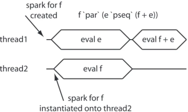
An execution trace for this program is shown in Figure 7.

thread1 eval f + e

eval f

f `par` (e `pseq` (f + e))

eval e

thread2

spark for f created

spark for f instantiated onto thread2

Fig. 7.A correct parallelization which is not dependent on the evaluation order of+

4.1 Weak Head Normal Form (WHNF)

(10)

1moduleMain 2where

3import System.Time 4importControl.Parallel 5

6fib ::Int−>Int 7fib 0 = 0 8fib 1 = 1

9fib n = fib (n−1) + fib (n−2) 10

11mapFib :: [Int]

12mapFib =mapfib [37, 38, 39, 40] 13

24sumEuler =sum. (mapeuler) . mkList 25

26mapEuler :: [Int]

27mapEuler =mapsumEuler [7600, 7600] 28

29parMapFibEuler ::Int

30parMapFibEuler = mapFib ‘par‘

31 (mapEuler ‘pseq‘ (summapFib +summapEuler)) 32

33main ::IO() 34main

35 =putStrLn(showparMapFibEuler)

The intention here is to compute two independent functions in parallel: – mapping thefibfunction over a list and then summing the result – mapping thesumEulerfunction over a list and the summing the result The main program then adds the two sums to produce the final result. We have chosen arguments which result in a similar run-time formapFib andmapEuler.

However, when we run this program with one and then two cores we observe no speedup:

satnams@MSRC-LAGAVULIN ~/papers/afp2008/whnf $ time WHNF2 +RTS -N1

(11)

real 0m48.086s user 0m0.000s

sys 0m0.015s

263935901

sys 0m0.015s

What went wrong? The problem is that the functionmapFib does not return a list with four values each fully evaluated to a number. Instead, the expression is reduced to weak head normal form which only return the top level cons cell with the head and the tail elements unevaluated as shown in Figure 8. This means that almost no work is done in the parallel thread. the root of the problem here is Haskell’s lazy evaluation strategy which comes into conflict with our desire to control what is evaluated when to help gain performance through parallel execution.

:

fib 37

map fib [38, 39, 40]

Fig. 8.parFibevaluated to weak head normal form (WHNF)

To fix this problem we need to somehow force the evaluation of the list. We can do this by defining a function that iterates over each element of the list and then uses each element as the first argument to pseq which will cause it to be evaluated to a number:

1forceList :: [a]−>() 2forceList [] = ()

3forceList (x:xs) = x ‘pseq‘ forceList xs

Using this function we can express our requirement to evaluate the mapFib function fully to a list of numbers rather than to just weak head normal form: 1moduleMain

2where

3importControl.Parallel 4

(12)

8fib n = fib (n−1) + fib (n−2) 9

10mapFib :: [Int]

11mapFib =mapfib [37, 38, 39, 40] 12

23sumEuler =sum. (mapeuler) . mkList 24

25mapEuler :: [Int]

26mapEuler =mapsumEuler [7600, 7600] 27

28parMapFibEuler ::Int

29parMapFibEuler = (forceList mapFib) ‘par‘

30 (forceList mapEuler ‘pseq‘ (summapFib +summapEuler)) 31

32forceList :: [a]−>() 33forceList [] = ()

34forceList (x:xs) = x ‘pseq‘ forceList xs 35

38 =putStrLn(showparMapFibEuler)

This gives the desired performance which shows the work ofmapFib is done in parallel with the work ofmapEuler:

263935901

sys 0m0.000s

263935901

(13)

sys 0m0.000s

Question. What would be the effect on performance if we omitted the call of forceListonmapEuler?

An important aspect of howpseqworks is that it evaluates its first argument to weak head normal formal. This does not fully evaluate an expression e.g. for an expression that constructs a list out of a head and a tail expression (a CONS expression)pseqwill not evaluate the head and tail sub-expressions.

Haskell also defines a function calledseqbut the compiler is free to swap the arguments of seq which means the user can not control evaluation order. The compiler has primitive support for pseq and ensures the arguments are never swapped and this function should always be preferred over seqfor parallel pro-grams.

4.2 Divide and conquer

Exercise 1: Parallel quicksort. The program below shows a sequential imple-mentation of a quicksort algorithm. Use this program as a template to write a parallel quicksort function. The main body of the program generates a pseudo-random list of numbers and then measures the time taken to build the input list and then to perform the sort and then add up all the numbers in the list. 1moduleMain

2where

3import System.Time 4importControl.Parallel 5import System.Random 6

7−−A sequential quicksort 8quicksort ::Orda=>[a]−>[a] 9quicksort [] = []

10quicksort (x:xs) = losort ++ x : hisort

11 where

12 losort = quicksort [y|y<−xs, y<x] 13 hisort = quicksort [y|y<−xs, y >= x] 14

15secDiff :: ClockTime−>ClockTime−>Float 16secDiff (TOD secs1 psecs1) (TOD secs2 psecs2)

17 =fromInteger(psecs2−psecs1) / 1e12 +fromInteger(secs2−secs1) 18

21 =dot0<−getClockTime

22 letinput = (take20000 (randomRs(0,100) (mkStdGen42)))::[Int] 23 seq(forceList input) (return())

24 t1<−getClockTime

25 letr =sum(quicksortF input)

(14)

28 −−Write out the sum of the result. 29 putStrLn(’’Sumof sort: ’’ ++showr)

30 −−Write out the time taken to perform the sort. 31 putStrLn(’’Time tosort: ’’ ++show(secDiff t1 t2))

The performance of a parallel Haskell program can sometimes be improved by reducing the number of garbage collections that occur during execution and a simple way of doing this is to increase the heap size of the program. The size of the heap is specified has an argument to the run-time system e.g. -K100M specifies a 100MB stack and-H800M means use a 800MB heap.

satnams@msrc-bensley /cygdrive/l/papers/afp2008/quicksort $ QuicksortD +RTS -N1 -H800M

Sum of sort: 50042651196 Time to sort: 4.593779

satnams@msrc-bensley /cygdrive/l/papers/afp2008/quicksort $ QuicksortD +RTS -N2 -K100M -H800M

Sum of sort: 50042651196 Time to sort: 2.781196

You should consider usingpar andpseqto try and compute the sub-sorts in parallel. This in itself may not lead to any performance improvement and you should then ensure that the parallel sub-sorts are indeed doing all the work you expect them to do (e.g. consider the effect of lazy evaluation). You may need to write a function toforcethe evaluation of sub-expressions.

You can get some idea of how well a program has been parallelized and how much time is taken up with garbage collection by using the runtime -s flag to dump some statistics to the standard output. We can also enable GHC’s parallel garbage collection and disable load balancing for better cache behaviour with the flags-qg0 -qb.

$ ./QuicksortD.exe +RTS -N2 -K100M -H300M -qg0 -qb -s

After execution of a parallel version of quicksort you can look at the end of the filen2.txtto see what happened:

.\QuicksortD.exe +RTS -N2 -K100M -H300M -qg0 -qb -s 1,815,932,480 bytes allocated in the heap

242,705,904 bytes copied during GC

55,709,884 bytes maximum residency (4 sample(s)) 8,967,764 bytes maximum slop

328 MB total memory in use (2 MB lost due to fragmentation)

Generation 0: 10 collections, 9 parallel, 1.62s, 0.83s elapsed Generation 1: 4 collections, 4 parallel, 1.56s, 0.88s elapsed

(15)

Task 0 (worker) : MUT time: 2.34s ( 3.55s elapsed) GC time: 0.91s ( 0.45s elapsed)

INIT time 0.00s ( 0.03s elapsed) MUT time 5.89s ( 3.58s elapsed) GC time 3.19s ( 1.70s elapsed) EXIT time 0.00s ( 0.02s elapsed) Total time 9.08s ( 5.31s elapsed)

%GC time 35.1% (32.1% elapsed)

Alloc rate 308,275,009 bytes per MUT second

Productivity 64.9% of total user, 110.9% of total elapsed This execution of quicksort spent 35.1% of its time in garbage collection. The work of the sort was shared out amongst two threads although not evenly. The MUT time gives an indication of how much time was spent performing compu-tation. Seven sparks were created and each of them was evaluated.

5 Explicit Concurrency

Writing semi-implicitly parallel programs can sometimes help to parallelize pure functional programs but it does not work when we want to parallelize stateful computations in the IO monad. For that we need to write explicitly threaded programs. In this section we introduce Haskell’s mechanisms for writing explic-itly concurrent programs. Haskell presents explicit concurrency features to the programmer via a collection of library functions rather than adding special syn-tactic support for concurrency and all the functions presented in this section are exported by this module.

5.1 Creating Haskell Threads

(16)

identi-fication of Haskell threads (which should not be confused with operating system threads). A new thread may be created for any computation in the IO monad which returns anIOunit result by calling theforkIO function:

1forkIO ::IO()−>IOThreadId

Why does the forkIO function take an expression in the IO monad rather than taking a pure functional expression as its argument? The reason for this is that most concurrent programs need to communicate with each other and this is done through shared synchronized state and these stateful operations have to be carried out in theIOmonad.

One important thing to note about threads that are created by callingforkIO is that the main program (the parent thread) will not automatically wait for the child threads to terminate.

Sometimes it is necessary to use a real operating system thread and this can be achieved using the forkOSfunction:

1forkOS ::IO()−>IOThreadId

Threads created by this call are bound to a specific operating system thread and this capability is required to support certain kinds of foreign calls made by Haskell programs to external code.

5.2 MVars

To facilitate communication and synchronization between threads Haskell pro-videsMVars (“mutable variables”) which can be used to atomically communicate information between threads.MVarsand their associated operations are exported by the moduleControl.Concurrent.MVar. The run-time system ensures that the op-erations for writing to and reading fromMVars occur atomically. AnMVarmay be empty or it may contain a value. If a thread tries to write to an occupied MVarit is blocked and it will be rewoken when theMVarbecomes empty at which point it can try again to atomically write a value into the MVar. If more than one thread is waiting to write to anMVarthen the system uses a first-in first-out scheme to wake up just the longest waiting thread. If a thread tries to read from an emptyMVarit is blocked and rewoken when a value is written into theMVar when it gets a chance to try and atomically read the new value. Again, if more than one thread is waiting to read from an MVarthe run-time system will only wake up the longest waiting thread.

Operations are provided to create an emptyMVar, to create a newMVarwith an initial value, to remove a value from anMVar, to observe the value in anMVar (plus non-blocking variants) as well as several other useful operations.

1dataMVar a 2

(17)

7readMVar :: MVar a−>IOa

8tryTakeMVar :: MVar a−>IO(Maybea) 9tryPutMVar :: MVar a−>a−>IO Bool 10isEmptyMVar :: MVar a−>IO Bool 11−−Plus other functions

One can use a pair ofMVars and the blocking operationsputMVarandtakeMVar to implement arendezvousbetween two threads.

1moduleMain 2where

3importControl.Concurrent 4importControl.Concurrent.MVar 5

6threadA :: MVarInt−>MVarFloat−>IO() 7threadA valueToSendMVar valueReceiveMVar 8 =do−− some work

9 −−now perform rendezvous by sending 72 10 putMVar valueToSendMVar 72−−send value 11 v<−takeMVar valueReceiveMVar

12 putStrLn(showv)

13

14threadB :: MVarInt−>MVarFloat−>IO() 15threadB valueToReceiveMVar valueToSendMVar 16 =do−− some work

17 −−now perform rendezvous by waiting on value 18 z<−takeMVar valueToReceiveMVar

19 putMVar valueToSendMVar (1.2∗z) 20 −−continue with other work 21

24 =doaMVar<−newEmptyMVar 25 bMVar<−newEmptyMVar 26 forkIO (threadA aMVar bMVar) 27 forkIO (threadB aMVar bMVar)

28 threadDelay 1000−− wait for threadA and threadB to finish (sleazy)

Exercise 2:Re-write this program to remove the use ofthreadDelayby using some other more robust mechanism to ensure the main thread does not complete until all the child threads have completed.

1moduleMain 2where

3importControl.Parallel 4importControl.Concurrent 5importControl.Concurrent.MVar 6

(18)

10fibThread ::Int−>MVarInt −>IO() 11fibThread n resultMVar

12 = putMVar resultMVar (fib n) 13

14sumEuler ::Int−>Int 15−−As before

16 17s1 ::Int

18s1 = sumEuler 7450 19

22 =do putStrLn”explicit SumFibEuler” 23 fibResult<−newEmptyMVar 24 forkIO (fibThread 40 fibResult) 25 pseq s1 (return())

26 f<−takeMVar fibResult

27 putStrLn(”sum: ” ++show(s1+f))

The result of running this program with one and two threads is: satnams@MSRC-1607220 ~/papers/afp2008/explicit

$ time ExplicitWrong +RTS -N1 explicit SumFibEuler

sum: 119201850

sys 0m0.031s

satnams@MSRC-1607220 ~/papers/afp2008/explicit $ time ExplicitWrong +RTS -N2

explicit SumFibEuler sum: 119201850

sys 0m0.015s

To fix this problem we must ensure the computation offibfully occurs inside thefibThreadthread which we do by usingpseq.

1moduleMain 2where

3importControl.Parallel 4importControl.Concurrent 5importControl.Concurrent.MVar 6

(19)

9

10fibThread ::Int−>MVarInt −>IO() 11fibThread n resultMVar

12 =dopseq f (return())−−Force evaluation in this thread 13 putMVar resultMVar f

14 where

15 f = fib n 16

17sumEuler ::Int−>Int 18−−As before

19 20s1 ::Int

21s1 = sumEuler 7450 22

25 =do putStrLn”explicit SumFibEuler” 26 fibResult<−newEmptyMVar 27 forkIO (fibThread 40 fibResult) 28 pseq s1 (return())

29 f<−takeMVar fibResult

30 putStrLn(”sum: ” ++show(s1+f))

Writing programs withMVars can easily lead to deadlock e.g. when one thread is waiting for a value to appear in anMVar but no other thread will ever write a value into that MVar. Haskell provides an alternative way for threads to syn-chronize without using explicit locks through the use ofsoftware transactional

memory(STM) which is accessed via the moduleControl.Concurrent.STM. A

sub-set of the declarations exposed by this module are shown below. 1dataSTM a−−A monad supporting atomic memory transactions

2atomically :: STM a−>IOa−−Perform a series of STM actions atomically 3retry :: STM a−−Retry current transaction from the beginning

4orElse :: STM a−>STM a −>STM a−−Compose two transactions

5dataTVar a−−Shared memory locations that support atomic memory operations 6newTVar :: a−>STM (TVar a)−−Create a new TVar with an initial value 7readTVar :: TVar a−>STM a−−Return the current value stored in a TVar 8writeTVar :: TVar a−>a−>STM ()−−Write the supplied value into a TVar

(20)

system does allow such parallel and interleaved execution through the use of a log which is used to roll back the execution of blocks that have conflicting views of shared information.

To execute an atomic block the function atomically takes a computation in theSTMmonad and executes it in theIOmonad.

To help provide a model for how STM works in Haskell an example is shown in Figures 9 and 10 which illustrates how two threads modify a shared variable using Haskell STM. It is important to note that this is just amodeland an actual implementation of STM is much more sophisticated.

Thread 1 tries to atomically increment a sharedTVar: 1 atomically (dov<−readTVar bal

2 writeTVar bal (v+1)

3 )

Thread 2 tries to atomically subtract three from a sharedTVar: 1 atomically (dov<−readTVar bal

2 writeTVar bal (v−3)

3 )

Figure 9(a) shows a shared variable bal with an initial value of 7 and two threads which try to atomically read and update the value of this variable. Thread 1 has an atomic block which atomically increments the value represented bybal. Thread 2 tries to atomically subtract 3 from the value represented bybal. Examples of valid executions include the case where (a) the value represented bybalis first incremented and then has 3 subtracted yielding the value 5; or (b) the case wherebalhas 3 subtracted and then 1 added yielding the value 6.

Figure 9(b) shows each thread entering its atomic block and a transaction log is created for each atomic block to record the initial value of the shared variables that are read and to record deferred updates to the shared variable which succeed at commit time if the update is consistent.

Figure 9(c) shows thread 2 reading a value of 7 from the shared variable and this read is recorded its local transaction log.

Figure 9(d) shows that thread 1 also observes a value of 7 from the shared variable which is stored in its transaction log.

Figure 9(e) shows thread 1 updating its view of the shared variable by incre-menting it by 1. This update is made to the local transaction log and not to the shared variable itself. The actual update is deferred until the transaction tries to commit when either it will succeed and the shared variable will be updated or it may fail in which case the log is reset and the transaction is re-run.

Figure 9(f) shows thread 2 updating its view of the shared variable to 4 (i.e. 7-3). Now the two threads have inconsistent views of what the value of the shared variable should be.

(21)

bal :: TVar Int

7

Thread 1

1 atomically (do

2 v <- readTVar bal

4 )

Thread 2

1 atomically (do

2 v <- readTVar bal

3 writeTVar bal (v-3)

4 )

bal :: TVar Int

7

Thread 1

1 atomically (do

2 v <- readTVar bal

4 )

Thread 2

1 atomically (do

2 v <- readTVar bal

4 )

What Value Read Value Written bal transaction log What Value Read Value Written bal transaction log

(a) Two threads each with an atomic block and one shared variable

(b) Both threads enter their atomic block and a log is created to track the use of bal

bal :: TVar Int

7

Thread 1

1 atomically (do

2 v <- readTVar bal

4 )

Thread 2

1 atomically (do

2 v <- readTVar bal

4 )

What Value Read Value Written bal transaction log What Value Read Value Written bal transaction log 7

(c) Thread 2 reads the value 7 from the shared variable and this read is recorded in its log

bal :: TVar Int

7

Thread 1

1 atomically (do

2 v <- readTVar bal

4 )

Thread 2

1 atomically (do

2 v <- readTVar bal

4 )

What Value Read Value Written bal transaction log What Value Read Value Written bal transaction log 7 7

(d) Thread 1 also reads the value 7 from the shared variable and this read is recorded in its log

bal :: TVar Int

7

Thread 1

1 atomically (do

2 v <- readTVar bal

4 )

Thread 2

1 atomically (do

2 v <- readTVar bal

4 )

What Value Read Value Written bal transaction log What Value Read Value Written bal transaction log 7 7 8

(e) Thread 1 updates its local view of the value of bal to 8 which is put in its own log

bal :: TVar Int

7

Thread 1

1 atomically (do

2 v <- readTVar bal

4 )

Thread 2

1 atomically (do

2 v <- readTVar bal

4 )

What Value Read Value Written bal transaction log What Value Read Value Written bal transaction log 7

7 8 4

(f) Thread 2 updates its local view of the value of bal to 4 which is put in its own log

bal :: TVar Int 8

Thread 1

1 atomically (do

2 v <- readTVar bal

4 )

Thread 2

1 atomically (do

2 v <- readTVar bal

4 )

What Value Read Value Written bal transaction log 7 4

• Thread1 commits • Shared bal variable is updated • Transaction log is discarded

(g) Thread 1 finoshes and updates the shared bal variable and discards its log.

bal :: TVar Int

8

Thread 1

1 atomically (do

2 v <- readTVar bal

4 )

Thread 2

1 atomically (do

2 v <- readTVar bal

4 )

What Value Read

Value Written

transaction log • Attempt to commit thread 2 fails,

because value in memory is not consistent with the value in the log • Transaction re-runs from the beginning

(h) Thread 2 tries to commit its changes which are now inconsistent with the updated value of bal

(22)

bal :: TVar Int

8

Thread 1

1 atomically (do

2 v <- readTVar bal

4 )

Thread 2

1 atomically (do

2 v <- readTVar bal

4 )

What Value Read Value Written transaction log 8 bal

(i) Thread 2 re-executes its atomic block from

the start, this time seeing a value of 8 for bal

bal :: TVar Int

8

Thread 1

1 atomically (do

2 v <- readTVar bal

4 )

Thread 2

1 atomically (do

2 v <- readTVar bal

4 )

What Value Read Value Written transaction log 8 bal 5

(j) Thread 2 updates it local value for bal

bal :: TVar Int

5

Thread 1

1 atomically (do

2 v <- readTVar bal

4 )

Thread 2

1 atomically (do

2 v <- readTVar bal

4 )

(k) Thread 2 now successfully commits its updates

Fig. 10.A model for STM in Haskell (continued)

is written in the shared value. These sequence of events occur atomically. Once the commit succeeds the transaction log is discarded and the program moves onto the next statement after the atomic block.

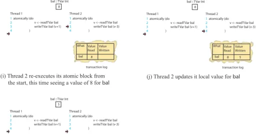
Figure 9(h) shows how the commit attempt made by thread 2 fails. This is because thread 2 has recorded a value of 7 forbalbut the actual value ofbal is 8. This causes the run-time system to erase the values in the log and restart the transaction which will cause it to see the updated value ofbal.

Figure 10(i) shows how thread 2 re-executes its atomic block but this time observing the value of 8 forbal.

Figure 10(j) shows thread 2 subtracting 3 from the recorded value ofbal to yield an updated value of 5.

Figure 10(k) shows that thread 2 can now successfully commit with an update of 5 to the shared variablebal. Its transaction log is discarded.

Theretryfunction allows the code inside an atomic block to abort the current transaction and re-execute it from the beginning using a fresh log. This allows us to implementmodular blocking. This is useful when one can determine that a transaction can not commit successfully. The code below shows how a transaction can try to remove money from an account with a case that makes the transaction re-try when there is not enough money in the account. This schedules the atomic block to be run at a later date when hopefully there will be enough money in the account.

1withdraw :: TVarInt−>Int−>STM () 2withdraw acc n

(23)

5 writeTVar acc (bal−n)

6 }

TheorElse function allows us to compose two transactions and allows us to implement the notion ofchoice. If one transaction aborts then the other transac-tion is executed. If it also aborts then the whole transactransac-tion is re-executed. The code below tries to first withdraw money from accounta1and if that fails (i.e. retry is called) it then attempts to withdraw money from account a2 and then it deposits the withdrawn money into account b. If that fails then the whole transaction is re-run.

1atomically (do{withdraw a1 3

2 ‘orElse‘

3 withdraw a2 3;

4 deposit b 3}

5 )

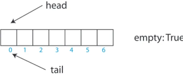
To illustrate the use of software transaction memory we outline how to rep-resent a queue which can be shared between Haskell threads. We shall reprep-resent a shared queue with a fixed sized array. A thread that writes to a queue that is full (i.e. the array is full) is blocked and a thread that tries to read from a queue that is empty (i.e. the array is empty) is also blocked. The data-type declaration below for an STM-based queue uses transactional variables to record the head element, the tail element, the empty status and the elements of the array that is used to back to queue.

1dataQueue e 2 = Queue

3 {shead :: TVarInt, 4 stail :: TVarInt, 5 empty :: TVarBool, 6 sa ::Array Int(TVar e) 7 }

A picture of an empty queue using this representation is shown in Figure 11.

head

tail

0

empty: True

1 2 3 4 5 6

Fig. 11.An empty queue

(24)

– Create a new empty queue by defining a function with the type: 1newQueue ::IO(Queue a)

– Add an element to the queue by defining a function with the type: enqueue :: Queue a−>a−>IO()

If the queue is full the caller should block until space becomes available and the value can be successfully written into the queue.

– Remove an element from the queue and return its value: dequeue :: Queue a−>IOa

If the queue is empty the caller should block until there is an item available in the queue for removal.

– Attempt to read a value from a queue and if it is empty then attempt to read a value from a different queue. The caller should block until a value can be obtained from one of the two queues.

dequeueEither :: Queue a−>Queue a−>IOa

6 Nested data parallelism

This chapter was written in collaboration with Manuel Chakravarty, Gabriele Keller, and Roman Leshchinskiy (University of New South Wales, Sydney).

The two major ways of exploiting parallelism that we have seen so far each have their disadvantages:

– The par/seq style is semantically transparent, but it is hard to ensure that the granularity is consistently large enough to be worth spawning new threads.

– Explicitly-forked threads, communicating usingMVars or STM give the pro-grammer precise control over granularity, but at the cost of a new layer of semantic complexity: there are now many threads, each mutating shared memory. Reasoning about all the inter leavings of these threads is hard, especially if there are a lot of them.

Furthermore, neither is easy to implement on a distributed-memory machine, be-cause any pointer can point to any value, so spatial locality is poor. It is possible to support this anarchic memory model on a distributed-memory architecture, as Glasgow Parallel Haskell has shown [3], but it is very hard to get reliable, predictable, and scalable performance. In short, we have no good performance model, which is a Bad Thing if your main purpose in writing a parallel program is to improve performance.

(25)

Do the same thing, in parallel, to every element of a large collection of values.

Not every program can be expressed in this way, but data parallelism is very attractive for those that can, because:

– Everything remains purely functional, likepar/seq, so there is no new se-mantic complexity.

– Granularity is very good: to a first approximation, we get just one thread (with its attendant overheads) for each physical processor, rather than one thread for each data item (of which there are zillions).

– Locality is very good: the data can be physically partitioned across the pro-cessors without random cross-heap pointers.

As a result, we get an excellent performance model.

6.1 Flat data parallelism

Data parallelism sounds good doesn’t it? Indeed, data-parallel programming is widely and successfully used in mainstream languages such as High-Performance Fortran. However, there’s a catch: the application has to fit the data-parallel programming paradigm, and only a fairly narrow class of applications do so. But this narrow-ness is largely because mainstream data-parallel technology only supports so-calledflat data parallelism. Flat data parallelism works like this

Apply the samesequential functionf, in parallel, to every element of a large collection of valuesa. Not only isfsequential, but it has a similar run-time for each element of the collection.

Here is how we might write such a loop in Data Parallel Haskell: sumSq :: [: Float :] -> Float

sumSq a = sumP [: x*x | x <- a :]

The data type[: Float :]is pronounced “parallel vector ofFloat”. We use a bracket notation reminiscent of lists, because parallel vectors are similar to lists in that consist of an sequence of elements. Many functions available for lists are also available for parallel vectors. For example

mapP :: (a -> b) -> [:a:] -> [:b:]

zipWithP :: (a -> b -> c) -> [:a:] -> [:b:] -> [:c:] sumP :: Num a => [:a:] -> a

(+:+) :: [:a:] -> [:a:] -> [:a:] filterP :: (a -> Bool) -> [:a:] -> [:a:] anyP :: (a -> Bool) -> [:a:] -> Bool concatP :: [:[:a:]:] -> [:a:]

nullP :: [:a:] -> Bool lengthP :: [:a:] -> Int

(26)

These functions, and many more, are exported byData.Array.Parallel. Just as we have list comprehensions, we also have parallel-array comprehensions, of which one is used in the above example. But, just as with list comprehensions, array comprehensions are syntactic sugar, and we could just as well have written

sumSq :: [: Float :] -> Float sumSq a = sumP (mapP (\x -> x*x) a)

Notice that there is no forkIO, and no par. The parallelism comes implicitly from use of the primitives operating on parallel vectors, such asmapP,sumP, and so on.

Flat data parallelism is not restricted to consuming a single array. For ex-ample, here is how we might take the product of two vectors, by multiplying corresponding elements and adding up the results:

vecMul :: [:Float:] -> [:Float:] -> Float vecMul a b = sumP [: x*y | x <- a | y <- b :]

The array comprehension uses a second vertical bar “|” to indicate that we interate over b in lockstep with a. (This same facility is available for ordinary list comprehensions too.) As before the comprehension is just syntactic sugar, and we could have equivalently written this:

vecMul :: [:Float:] -> [:Float:] -> Float vecMul a b = sumP (zipWithP (*) a b)

6.2 Pros and cons of flat data parallelism

If you can express your program using flat data parallelism, we can implement it really well on a N-processor machine:

– Divideainto N chunks, one for each processor.

– Compile a sequential loop that applies fsuccessively to each element of a chunk

– Run this loop on each processor – Combine the results.

Notice that the granularity is good (there is one large-grain thread per proces-sor); locality is good (the elements ofaare accessed successively); load-balancing is good (each processor does 1/Nof the work). Furthermore the algorithm works well even iff itself does very little work to each element, a situation that is a killer if we spawn a new thread for each invocation off.

In exchange for this great implementation, the programming model is hor-rible: all the parallelism must come from a single parallel loop. This restriction makes the programming model is very non-compositional. If you have an existing function gwritten using the data-parallel mapP, you can’t call g from another data-parallel map (e.g. mapP g a), because the argument to mapP must be a

(27)

Furthermore, just as the control structure must be flat, so must the data structure. We cannot allowato contain rich nested structure (e.g. the elements of acannot themselves be vectors), or else similar-run-time promise of fcould not be guaranteed, and data locality would be lost.

6.3 Nested data parallelism

In the early 90’s, Guy Blelloch describednesteddata-parallel programming. The idea is similar:

Apply the same functionf, in parallel, to every element of a large col-lection of values a. However, f may itself be a (nested) data-parallel function, and does not need to have a similar run-time for each element ofa.

For example, here is how we might multiply a matrix by a vector: type Vector = [:Float:]

type Matrix = [:Vector:]

matMul :: Matrix -> Vector -> Vector matMul m v = [: vecMul r v | r <- m :]

That is, for each row of the matrix, multiply it by the vector v using vecMul. Here we are calling a data-parallel function vecMul from inside a data-parallel operation (the comprehension inmatMul).

In very regular examples like this, consisting of visible, nested loops, modern FORTRAN compilers can collapse a loop nest into one loop, and partition the loop across the processors. It is not entirely trivial to do this, but it is well within the reach of compiler technology. But the flattening process only works for the simplest of cases. A typical complication is the matrices may besparse.

A sparse vector (or matrix) is one in which almost all the elements are zero. We may represent a sparse vector by a (dense) vector of pairs:

type SparseVector = [: (Int, Float) :]

In this representation, only non-zero elements of the vector are represented, by a pair of their index and value. A sparse matrix can now be represented by a (dense) vector of rows, each of which is a sparse vector:

type SparseMatrix = [: SparseVector :]

Now we may writevecMulandmatMulfor sparse arguments thus1

: 1

Incidentally, although these functions are very short, they are important in some applications. For example, multiplying a sparse matrix by a dense vector (i.e.

(28)

sparseVecMul :: SparseVector -> Vector -> Float sparseVecMul sv v = sumP [: x * v!:i | (i,x) <- sv :]

sparseMatMul :: SparseMatrix -> Vector -> Vector sparseMatMul sm v = [: sparseVecMul r v | r <- sm :]

We use the indexing operator (!:) to index the dense vector v. In this code, the control structure is the same as before (a nested loop, with both levels being data-parallel), but now the data structure is much less regular, and it is much

less obvious how to flatten the program into a single data-parallel loop, in such a way that the work is evenly distributed over N processors, regardless of the distribution of non-zero data in the matrix.

Blelloch’s remarkable contribution was to show that it is possible to take

any program written using nested data parallelism (easy to write but hard to implement efficiently), and transform it systematically into a program that uses flat data parallelism (hard to write but easy to implement efficiently). He did this for a special-purpose functional language, NESL, designed specifically to demonstrate nested data parallelism.

As a practical programming language, however, NESL is very limited: it is a first-order language, it has only a fixed handful of data types, it is im-plemented using an interpreter, and so on. Fortunately, in a series of papers, Manuel Chakravarty, Gabriele Keller and Roman Leshchinskiy have generalized Blelloch’s transformation to a modern, higher order functional programming language with user-defined algebraic data types – in other words, Haskell. Data Parallel Haskell is a research prototype implementation of all these ideas, in the Glasgow Haskell Compiler, GHC.

The matrix-multiply examples may have suggested to you that Data Parallel Haskell is intended primarily for scientific applications, and that the nesting depth of parallel computations is statically fixed. However the programming paradigm is much more flexible than that. In the rest of this chapter we will give a series of examples of programming in Data Parallel Haskell, designed to help you gain familiarity with the programming style.

Most (in due course, all) of these examples can be found at in the Darcs repos-itoryhttp://darcs.haskell.org/packages/ndp, in the sub-directoryexamples/. You can also find a dozen or so other examples of data-parallel algorithms written in NESL at_{http://www.cs.cmu.edu/~scandal/nesl/algorithms.html}.

6.4 Word search

Here is a tiny version of a web search engine. A Documentis a vector of words, each of which is a string. The task is to find all the occurrences of a word in a large collection of documents, returning the matched documents and the matching word positions in those documents. So here is the type signature for search:

(29)

type DocColl = [: Document :]

search :: DocColl -> String -> [: (Document, [:Int:]) :]

We start by solving an easier problem, that of finding all the occurrences of a word in a single document:

wordOccs :: Document -> String -> [:Int:]

wordOccs d s = [: i | (i,s2) <- zipP [:1..lengthP d:] d , s == s2 :]

Here we use a filter in the array comprehension, that selects just those pairs (i,s2) for which s==s2. Because this is an array comprehension, the implied filtering is performed in data parallel. The(i,s2)pairs are chosen from a vector of pairs, itself constructed by zipping the document with the vector of its indices. The latter vector [: 1..lengthP d :] is again analogous to the list notation [1..n], which generate the list of values between 1and n. As you can see, in both of these cases (filtering and enumeration) Data Parallel Haskell tries hard to make parallel arrays and vectors as notationally similar as possible.

With this function in hand, it is easy to buildsearch:

search :: [: Document :] -> String -> [: (Document, [:Int:]) :] search ds s = [: (d,is) | d <- ds

, let is = wordOccs d s , not (nullP is) :]

6.5 Prime numbers

Let us consider the problem of computing the prime numbers up to a fixed numbern, using the sieve of Erathosthenes. You may know the cunning solution using lazy evaluation, thus:

primes :: [Int]

primes = 2 : [x | x <- [3..]

, not (any (‘divides‘ x) (smallers x))] where

smallers x = takeWhile (\p -> p*p <= x) primes

divides :: Int -> Int -> Bool divides a b = b ‘mod‘ a == 0

(In fact, this code is not the sieve of Eratosthenes, as Melissa O’Neill’s elegant article shows [5], but it will serve our purpose here.) Notice that when considering a candidate primex, we check that is is not divisible by any prime smaller than the square root ofx. This test involves usingprimes, the very list the definition produces.

(30)

primesUpTo :: Int -> [: Int :] primesUpTo 1 = [: :]

primesUpTo 2 = [: 2 :] primesUpTo n = smallers +:+

[: x | x <- [: ns+1..n :]

, not (anyP (‘divides‘ x) smallers) :] where

ns = intSqrt n

smallers = primesUpTo ns

As in the case of wordOccs, we use a boolean condition in a comprehension to filter the candidate primes. This time, however, computing the condition itself is a nested data-parallel computation (as it was in search). used here to filter candidate primes x.

To computesmallerswe make a recursive call toprimesUpTo. This makes primesUpTounlike all the previous examples: the depth of data-parallel nesting is determineddynamically, rather than being statically fixed to depth two. It should be clear that the structure of the parallelism is now much more complicated than before, and well out of the reach of mainstream flat data-parallel systems. But it has abundant data parallelism, and will execute with scalable performance on a parallel processor.

6.6 Quicksort

In all the examples so far the “branching factor” has been large. That is, each data-parallel operations has worked on a large collection. What happens if the collection is much smaller? For example, a divide-and-conquer algorithm usually divides a problem into a handful (perhaps only two) sub-problems, solves them, and combines the results. If we visualize the tree of tasks for a divide-and-conquer algorithm, it will have a small branching factor at each node, and may be highly un-balanced.

Is this amenable to nested data parallelism? Yes, it is. Quicksort is a classic divide-and-conquer algorithm, and one that we have already studied. Here it is, expressed in Data Parallel Haskell:

qsort :: [: Double :] -> [: Double :] qsort xs | lengthP xs <= 1 = xs

| otherwise = rs!:0 +:+ eq +:+ rs!:1 where

p = xs !: (lengthP xs ‘div‘ 2) lt = [:x | x <- xs, x < p :] eq = [:x | x <- xs, x == p:] gr = [:x | x <- xs, x > p :] rs = mapP qsort [: lt, gr :]

(31)

only two elements in the vector does not matter. If you visualize the binary tree of sorting tasks that quicksort generates, then each horizontal layer of the tree is done in data-parallel, even though each layer consists of many unrelated sorting tasks.

6.7 Barnes Hut

All our previous examples worked on simple flat or nested collections. Let’s now have a look at an algorithm based on a more complex structure, in which the elements of a parallel array come from a recursive and user-defined algebraic data type.

In the following, we present an implementation2

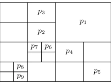
of a simple version of the Barnes-Hutn-body algorithm[7], which is a representative of an important class of parallel algorithms covering applications like simulation and radiocity compu-tations. These algorithms consist of two main steps: first, the data is clustered in a hierarchical tree structure; then, the data is traversed according to the hi-erarchical structure computed in the first step. In general, we have the situation that the computations that have to be applied to data on the same level of the tree can be executed in parallel. Let us first have a look at the Barnes-Hut al-gorithm and the data structures that are required, before we discuss the actual implementation in parallel Haskell.

Ann-body algorithm determines the interaction between a set of particles by computing the forces which act between each pair of particles. A precise solution therefore requires the computations ofn2

forces, which is not feasible for large numbers of particles. The Barnes-Hut algorithm minimizes the number of force calculations by grouping particles hierarchically intocellsaccording to their spa-tial position. The hierarchy is represented by a tree. This allows approximating the accelerations induced by a group of particles on distant particles by using the centroid of that group’s cell. The algorithm has two phases: (1) The tree is constructed from a particle set, and (2) the acceleration for each particle is computed in a down-sweep over the tree. Each particle is represented by a value of typeMassPoint, a pair of position in the two dimensional space and mass:

type Vec = (Double, Double) type Area = (Vec, Vec) type Mass = Double type MassPoint = (Vec, Mass)

We represent the tree as a node which contains the centroid and a parallel array of subtrees:

data Tree = Node MassPoint [:Tree:]

Notice that aTreecontains a parallel array of Tree.

Each iteration ofbhTreetakes the current particle set and the area in which the particles are located as parameters. It first splits the area into four subareas

2

(32)

p6 p7

p4 p5 p2

p3

p8 p9

p1

Fig. 12.Hierarchical division of an area into subareas

subAsof equal size. It then subdivides the particles into four subsets according to the subarea they are located in. Then,bhTreeis called recursively for each subset and subarea. The resulting four trees are the subtrees of the tree representing the particles of the area, and the centroid of their roots is the centroid of the complete area. Once an area contains only one particle, the recursion terminates. Figure 12 shows such a decomposition of an area for a given set of particles, and Figure 13 displays the resulting tree structure.

bhTree :: [:MassPnt:] -> Area -> Tree bhTree p area = Node p [::]

bhTree ps area = let

subAs = splitArea area

pgs = splitParticles ps subAs

subts = [: bhTree pg a| pg <- pgs | a <- subAs :] cd = centroid [:mp | Node mp _ <- subts :] in Node cd subts

The tree computed by bhTreeis then used to compute the forces that act on each particle by a function accels. It first splits the set of particles into two subsets: fMps, which contains the particles far away (according to a given criteria), and cMps, which contains those close to the centroid stored in the root of the tree. For all particles in fMps, the acceleration is approximated by computing the interaction between the particle and the centroid. Then,accels is called recursively for with cMps and each of the subtrees. The computation terminates once there are no particles left in the set.

accels:: Tree -> [:MassPoint:] -> [:Vec:]

accels _ [::] = [::]

accels (Node cd subts) mps = let

(fMps, cMps) = splitMps mps

(33)

p6 p7 p8 p9

c4 c5 p2 p3 p4 p5

c1 c2 c3 p1

c0

Fig. 13.Example of a Barnes-Hut tree.

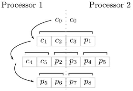
Processor 1 Processor 2

c0 c0 c1 c2 c3 p1 c4 c5 p2 p3 p4 p5

p5 p6 p7 p8

Fig. 14.Distribution of the values of the flattened tree

accel :: MassPoint -> MassPoint -> Vec

-- Given two particles, the function accel computes the -- acceleration that one particle exerts on the other

The tree is both built and traversed level by level, i.e., all nodes in one level of the tree are processed in a single parallel step, one level after the other. This information is important for the compiler to achieve good data locality and load balance, because it implies that each processor should have approximately the same number of masspoints of each level. We can see the tree as having a se-quential dimension to it, its depth, and a parallel dimension, the breadth, neither of which can be predicted statically. The programmer conveys this information to the compiler by the choice the data structure: By putting all subtrees into a parallel array in the type definition, the compiler assumes that all subtrees are going to be processed in parallel. The depth of the tree is modeled by the recursion in the type, which is inherently sequential.

6.8 A performance model

(34)

First, we must make explicit something we have glossed over thus far: data-parallel arrays are strict. More precisely, if any element of a data-parallel array di-verges, then all elements diverge3

. This makes sense, because if we demand any element of a parallel array then we must compute them all in data parallel; and if that computation diverges we are justified in not returning any of them. The same constraint means that we can represent parallel arrays very efficiently. For example, an array of floats, [:Float:], is represented by a contiguous array of unboxed floating-point numbers. There are no pointers, and iterating over the array has excellent spatial locality.

In reasoning about performance, Blelloch [9] characterizes theworkanddepth

of the program:

– Thework,W, of the program is the time it would take to execute on a single processor.

– The depth, D, of the program is the time it would take to execute on an

infinite number processors, under the assumption that the additional pro-cessors leap into action when (but only when) amapP, or other data-parallel primitive, is executed.

If you think of the unrolled data-flow diagram for the program, the work is the number of nodes in the data-flow diagram, while the depth is the longest path from input to output.

Of course, we do not have an infinite number of processors. Suppose instead that we have P processors. Then if everything worked perfectly, the work be precisely evenly balanced across the processors and the execution timeT would beW/P. That will not happen if the depthDis very large. So in fact, we have

W/P ≤T ≤W/P+L∗D

where L is a constant that grows with the latency of communication in the machine. Even this is a wild approximation, because it takes no account of bandwidth limitations. For example, between each of the recursive calls in the Quicksort example there must be some data movement to bring together the elements less than, equal to, and greater than the pivot. Nevertheless, if the net-work bandwidth of the parallel machine is high (and on serious multiprocessors it usually is) the model gives a reasonable approximation.

How can we compute work and depth? It is much easier to reason about the work of a program in a strict setting than in a lazy one, because all sub-expressions are evaluated. This is why the performance model of the data-parallel part of DPH is more tractable than for Haskell itself.

The computation of depth is where we take account of data parallelism. Figure 15 shows the equations for calculating the depth of a closed expression

e, where D[[e]] means “the depth of e”. These equations embody the following ideas:

– By default execution is sequential. Hence, the depth of an addition is the sum of the depths of its arguments.

3

(35)

D[[k]] = 0 wherekis a constant

D[[x]] = 0 wherexis a variable

D[[e1+e2]] = 1 +D[[e1]] +D[[e2]]

D[[ife1 thene2 elsee3]] =D[[e1]] +D[[e2]] ife1=True

=D[[e1]] +D[[e3]] ife1=False D[[letx=einb]] =D[[b[e/x]]]

D[[e1 +:+e2]] = 1 +D[[e1]] +D[[e2]] D[[concatPe]] = 1 +D[[e]]

D[[mapPf e]] = 1 +D[[e]] +maxx∈e D[[f x]]

D[[filterPf e]] = 1 +D[[e]] +D[[f]]

D[[sumPe]] = 1 +D[[e]] +log(length(e))

Fig. 15.Depth model for closed expressions

– The parallel primitive mapP, and its relatives such as filterP, can take advantage of parallelism, so the depth is the worst depth encountered for any element.

– The parallel reduction primitivesumP, and its relatives, take time logarithmic in the length of the array.

The rule for mapP dirctly embodies the idea that nested data parallelism is flattened. For example, suppose e :: [:[:Float:]:]. Then, applying the rules we see that

D[[mapPf (concatPe]] = 1 +D[[concatPe]] +_x∈concatPmax _eD[[f x]]

= 1 + 1 +D[[e]] +_x∈concatPmax _eD[[f x]]

= 2 +D[[e]] +max_xs∈e maxx∈xsD[[f x]] D[[mapP(mapPf)e]] = 1 +D[[e]] +maxxs∈eD[[mapPf xs]]

= 1 +D[[e]] + 1 +max_xs∈e maxx∈xsD[[f x]]

= 2 +D[[e]] +max_xs∈e maxx∈xsD[[f x]]

Notice that although the second case is a nested data-parallel computation, it has the same depth expression as the first: the data-parallel nesting is flattened. These calculations are obviously very approximate, certainly so far as con-stant factors are concerned. For example, in the inequality for execution time,

W/P ≤T ≤W/P+L∗D

(36)

A program has the Asymptotic Scalability property ifD grows asymp-totically more slowly thanW, as the size of the problem increases.

If this is so then, for a sufficiently large problem and assuming sufficient network bandwidth, performance should scale linearly with the number of processors.

For example, the functionssumSqandsearchboth have constant depth, so both have the AS property, and (assuming sufficient bandwidth) performance should scale linearly with the number of processors after some fairly low thresh-old.

For Quicksort, an inductive argument shows that the depth is logarithmic in the size of the array, assuming the pivot is not badly chosen. SoW =O(nlogn) andD=O(logn), and Quicksort has the AS property.

For computing primes, the depth is smaller:D=O(loglogn). Why? Because at every step we take the square root ofn, so that at depthdwe haven= 22d

. Almost all the work is done at the top level. The work at each level involves comparing all the numbers between√nandnwith each prime smaller than√n. There are approximately√n/lognprimes smaller than√n, so the total work is roughly W =O(n3/2

/logn). So again we have the AS property. Leshchinskiyet al [10] give further details of the cost model.

6.9 How it works

NESL’s key insight is that it is possible to transform a program that usesnested

data-parallelism into one that uses only flat data parallelism. While this little miracle happens behind the scenes, it is instructive to have some idea how it works, just as a car driver may find some knowledge of internal combustion engines even if he is not a skilled mechanic. The description here is necessarily brief, but the reader may find a slightly more detailed overview in [11], and in the papers cited there.

We call the nested-to-flat transformation thevectorizationtransform. It has two parts:

– Transform the data so that all parallel arrays contain only primitive, flat data, such asInt,Float,Double.

– Transform thecode to manipulate this flat data.

To begin with, let us focus on the first of these topics. We may consider it as the driving force, because nesting of data-parallel operations is often driven by nested data structures.

Transforming the data As we have already discussed, a parallel array of Floatis represented by a contiguous array of honest-to-goodness IEEE floating point numbers; and similarly forIntandDouble. It is as if we could define the parallel-array type by cases, thus:

(37)

In each case the Intfield is the size of the array. These data declarations are unusual because they arenon-parametric: the representation of an array depends on the type of the elements4

.

Matters become even more interesting when we want to represent a parallel array of pairs. We must not represent it as a vector of pointers to heap-allocated pairs, scattered randomly around the address space. We get much better locality if we instead represent it as apair of arrays thus:

data instance [: (a,b) :] = PP [:a:] [:b:]

Note that elements of vectors are hyperstrict. What about a parallel array of parallel arrays? Again, we must avoid a vector of pointers. Instead, the natural representation is obtained by literally concatenating the (representation of) the sub-vectors into one giant vector, together with a vector of indices to indicate where each of the sub-vectors begins.

data instance [: [:a:] :] = PA [:Int:] [:a:]

By way of example, recall the data types for sparse matrices: type SparseMatrix = [: SparseVector :]

type SparseVector = [: (Int, Float) :]

Now consider this tiny matrix, consisting of two short documents: m :: SparseMatrix

m = [: [:(1,2.0), (7,1.9):], [:(3,3.0):] :]

This would be represented as follows: PA [:0,2:] (PP [:1, 7, 3 :]

[:1.0, 1.9, 3.0:])

The array (just like the leaves) are themselves represented as byte arrays: PA (PI 2 #<0x0,0x2>)

(PP (PI 3 #<0x1, 0x7, 0x3>) (PF 3 #<0x9383, 0x92818, 0x91813>))

Here we have invented a fanciful notation for literalByteArrays (not supported by GHC, let alone Haskell) to stress the fact that in the end everything boils down to literal bytes. (The hexadecimal encodings of floating point numbers are also made up because the real ones have many digits!)

We have not discussed how to represent arrays of sum types (such asBool, Maybe, or lists), nor of function types — see [14] and [8] respectively.

4

None of this is visible to the programmer, but the data instance notation is in fact available to the programmer in recent versions of GHC [12, 13]. Why? Because GHC has a typed intermediate language so we needed to figure out how to give a