www.hydrol-earth-syst-sci.net/11/1309/2007/ © Author(s) 2007. This work is licensed under a Creative Commons License.
Earth System
Sciences
Exploratory data analysis and clustering of multivariate spatial
hydrogeological data by means of GEO3DSOM, a variant of
Kohonen’s Self-Organizing Map
L. Peeters1, F. Bac¸˜ao2, V. Lobo2,3, and A. Dassargues1,4 1Applied Geology and Mineralogy, KULeuven, Belgium
2Instituto Superior de Estat´ıstica e Gest˜ao de Informac¸˜ao, Universidade Nova de Lisboa, Campus de Campolide, Lisboa,
Portugal
3Portuguese Naval Academy, Almada, Portugal
4Hydrogeology & Environmental Geology, ArGEnCo, University of Liege, Belgium
Received: 17 May 2006 – Published in Hydrol. Earth Syst. Sci. Discuss.: 11 July 2006 Revised: 16 March 2007 – Accepted: 24 April 2007 – Published: 11 May 2007
Abstract. The use of unsupervised artificial neural network techniques like the self-organizing map (SOM) algorithm has proven to be a useful tool in exploratory data analysis and clustering of multivariate data sets. In this study a vari-ant of the SOM-algorithm is proposed, the GEO3DSOM, capable of explicitly incorporating three-dimensional spa-tial knowledge into the algorithm. The performance of the GEO3DSOM is compared to the performance of the stan-dard SOM in analyzing an artificial data set and a hydro-chemical data set. The hydrohydro-chemical data set consists of 131 groundwater samples collected in two detritic, phreatic, Cenozoic aquifers in Central Belgium. Both techniques suc-ceed very well in providing more insight in the groundwater quality data set, visualizing the relationships between vari-ables, highlighting the main differences between groups of samples and pointing out anomalous wells and well screens. The GEO3DSOM however has the advantage to provide an increased resolution while still maintaining a good general-ization of the data set.
1 Introduction
Regional monitoring of groundwater quality often yields large multidimensional data sets in which each sampling lo-cation is characterized by its geographic coordinates, longi-tude, latitude and height. Exploratory data analysis (EDA) and clustering can help in summarizing available data, ex-tracting useful information and formulating hypothesis for further research.
Correspondence to:L. Peeters ([email protected])
Traditionally multivariate techniques like principal com-ponent analysis (PCA) and factor analysis (FA) are used in the process of exploratory data analysis and clustering (e.g. G¨uler et al., 2002; Lambrakis et al., 2004; Love et al., 2004). Both PCA and FA are based on linear combinations of the original variables in order to reduce the dimensionality of the data set (Davis, 1986).
Recently, artificial neural network techniques, such as Ko-honen’s Self-Organizing Map (SOM), have also been used in EDA. The Self-Organizing Map may be used to project mul-tidimensional data onto a two dimensional grid in a topology preserving way, capturing complex, non-linear relationships between variables (Kohonen, 1995).
Besides applications of the algorithm in financial, medical, chemical and biological research (an overview is presented in Kaski, 1997), SOM’s are also used in remote sensing (Richardson et al., 2003; Mercier et al., 2006), geophysics (Poulton et al., 1992; Ozerdem et al., 2006), geochemistry (Lacassie et al., 2004; Penn, 2005) and reservoir charac-terization (Chang et al., 2002). Applications of the SOM-algorithm in hydrogeological research can be found in Hong and Rosen (2001) where technique is applied to diagnose the effect of storm water infiltration on groundwater quality vari-ables and to capture the complex nonlinear relationships be-tween groundwater quality variables. Sanchez-Martos et al. (2002) used SOM in the classification of a hydrochemical data set from a detritic aquifer in a semi-arid region, into distinct classes of different chemical composition. Lischeid (2003) applied the self-organizing map algorithm to an inten-sively monitored watershed to investigate spatial and tempo-ral trends in water quality data.
clustering of geospatial data and numerous applications of the technique in geospatial data analysis have proven to be successful (Takatsuka, 2001; Skupin and Hagelman, 2003; Koua et al., 2006). However, the inclusion of spatial or-dering in the clustering or classification algorithm remains an important issue, especially in hydrogeochemical research. The chemical composition of groundwater at a certain lo-cation can be thought of as the result of geochemical pro-cesses combined with groundwater flow related phenomena as mixing, advection and diffusion. In aquifers these pro-cesses seldom result in abrupt changes in hydrochemistry, but rather show a gradual change. Based on the premise that samples located close together are more likely to be related to each other than samples with a large distance between them, the incorporation of geographical coordinates in the EDA-algorithm provides a way of accounting for the spa-tial correlation in the exploratory data analysis. Bac¸˜ao et al. (2005a) discusses this topic in relation to the SOM-algorithm and compares the standard SOM-analysis in which the geo-graphic coordinates are considered as any other variable to the GEOSOM, a modified version of the SOM, designed to explicitly incorporate spatial information. Application of the GEOSOM on two artificial data sets and a real-world demo-graphic data set revealed the ability of the GEOSOM to in-crease the spatial resolution of the clustering.
The GEO-SOM as presented by Bac¸˜ao et al. (2005a) is limited to two-dimensional geo-referenced data. In this study, the GEOSOM is extended to incorporate three-dimensional geo-referenced data, hence the name GEO3DSOM. The objective of the GEO3DSOM algorithm is to extent the exploratory data analysis capabilities of the standard SOM to incorporate the geographic location of the samples in three dimensions, based on the premise that sam-ples located in each others vicinity are likely to be related to each other. A thorough discussion on the algorithms pro-posed is presented in the next section. Comparison between the standard SOM and the GEO3DSOM is carried out by applying both techniques to a theoretical data set and a hy-drochemical data set from two phreatic, sandy aquifers in Central Belgium.
2 Methods
2.1 Standard SOM
Artificial Neural Networks (ANN) are computer algorithms, inspired by the functioning of the nervous system of the hu-man brain, capable of learning from data and generalizing. This learning process can be described as supervised or un-supervised learning. In the un-supervised learning process, the ANN is shown several input-output patterns during training to enable the trained ANN to make generalizations based on the training data and to correctly produce output patterns based on new input (Jain et al., 1996). Neural networks are
widely applied in hydrologic research (e.g. ASCE, 2000), es-pecially in time-series prediction (e.g. Coppola et al., 2003; Alvisi et al., 2006)
The SOM-algorithm is based on unsupervised learning, which means that the desired output is not known a priori. The goal of the learning process is not to make predictions, but to classify data according to their similarity. In the early 1980s Kohonen proposed a neural network architecture in which the classification is done by plotting the data in n-dimensions onto a, usually, two-dimensional grid of units in a topology-preserving manner (Kohonen, 1995). The for-mer means that similar observations are plotted in each others neighborhood on the 2-D-grid. The network architecture and the learning algorithm are illustrated in Fig. 1.
The neural network consists of an input layer and a layer of neurons. The neurons or units are arranged on a rectangu-lar or hexagonal grid and are fully interconnected. Each of the input vectors is also connected to each of the units. The learning algorithm applied to the network can be divided into six steps (Kohonen, 1995; Kaski, 1997):
1. Anm×nmatrix is created from the data set withmrows of samples andncolumns of variables. The matrix thus consists ofminput vectors of lengthn. The classifica-tion of the input vectors is based on a similarity mea-surement, for instance Euclidean distance. In order to avoid bias in classification due to differences in mea-suring unit or range of the variables, a normalization is carried out. This can be done by setting mean equal to zero and variance equal to 1 or by rescaling the range of each variable in the[0,1]interval.
2. Each unit is randomly assigned an initial weight or ref-erence vector with a length equal to the length of the input vectors (n).
3. An input vector is shown to the network; the Euclidean distances between the considered input vectorXand all of the reference vectorsMi are calculated according to: X=(x1, x2, . . . , xn)∈Rn
M=(m1, m2, . . . , mn)∈Rn
kX−Mk = v u u t
n X
i=1
(xi −mi)2 (1)
4. The best matching unit Mc, the unit with the greatest similarity with the considered input vector, is chosen according to:
kX−Mck =min
i {kX−Mik} (2)
5. The weights of the best matching unit and the unit within its neighborhood N (t ) are adapted so that the new reference vectors lie henceforth closer to the input vector. The factorα(t )controls the rate of change of the reference vectors and is called the learning rate.
Mi(t+1)=
Mi(t )+α(t )[X(t )−Mi(t )] ∀∈N (t )
Mi(t ) ∀∈/N (t ) (3)
This is illustrated in Fig. 1c where the weights of the upper left unit and the units within the neighborhood N (t ) with radius r, indicated by the dashed line, are adapted. The rate of adaptation of the units is controlled by the neighborhood functionh, which decreases from one at the winning unit to zero at units located farther away than radiusr. The most common used functions are bell-shaped (Gaussian) or square (bubble).
6. Steps 3 until 5 are repeated until a predefined maximum number of iterations is reached. During these iterations bothαandN (t )decrease, forcing the network to con-verge.
After training, each of the input vectors is assigned to its best matching unit and the grids can be visualized. There are two types of grids commonly used to visualize and ana-lyze the result of the SOM procedure: component planes and U-matrix (Vesanto et al., 1999). The U-matrix or distance matrix shows the Euclidean distance between neighboring units by means of a grey scale. Typically darker colors rep-resent great distances and lighter shades reprep-resent small dis-tances. In this visualization method clusters are represented by a light area with darker borders, meaning that the refer-ence vectors in a cluster and the input vectors assigned to them are more similar to each other than to reference vec-tors outside the cluster. Additionally the labels of the input vectors can be plotted onto the U-matrix to identify the input vectors forming a cluster.
The component planes are the second visualization tech-nique. In these maps the component values of the weight vectors are represented by a color code. Each of the compo-nent planes visualizes the distribution of one variable in the data set (Ultsch and Herrmann, 2005). By visually compar-ing those maps, variables with similar distributions can be detected and it helps in visually finding correlations between variables.
The Self-Organizing Map algorithm is closely related to K-means clustering. A SOM with a number of units equal to the number of clusters in the data set and a neighborhood equal to zero will act as a traditional clustering technique (Kaski, 1997). A SOM may, however, be used in two very distinct ways: a large SOM, also known as emergent SOM, with many units, used for exploratory data analysis and clus-ter detection (Ultsch and Herrmann, 2005), and a small SOM for cluster centroid determination (Bac¸˜ao et al., 2005b). In
(0;0;0)
(0;0.5;0)
(0;1;0)
(0.5;0;0)
(0.5;0.5; 0.5)
(0.5;1; 0.5)
(1;0;0)
(1;0.5;1)
(1;1;1)
a
b
c
inputv
ector
inputv
ector
inputv
ector
(0;0.1;0.02)
0.102
0.400
0.900
0.510
0.800
1.136
1.001
1.456
1.664
Nor
malisation
(0;0.1; 0.05)
(0;0.25; 0)
(0;1;0)
(0.25;0; 0)
(0.4;0.4; 0.4)
(0.5;1; 0.5)
(1;0;0)
(1;0.5;1)
(1;1;1)
Nor
malisation
Nor
malisation
N(t)
Fig. 1.SOM-algorithm
(a)Initialization reference vectors of the units
(b)Calculation of Euclidean distance between input vector and
ref-erence vectors of the units
(c)Assignment of input vector to its BMU and update of reference
X
Y
Z
1
0.1 1
0.1 1
D=1
D=0
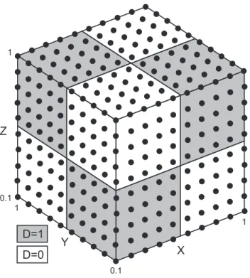
Fig. 2.Theoretical dataset.
this study, both SOM and GEO3DSOM are used for ex-ploratory detection of clusters. When using K-means and fuzzy C-means-clustering, cluster centroids will always be detected based on the objective criterium of sum-of-squared distances. In emergent SOM’s on the other hand, clearly sep-arated groups of units may or may not be detected. Small SOM’s used for centroid determination will act as a robust K-means initialization in the first training iterations and due to the decrease of learning radius and neighborhood during training, the SOM will perform exactly as a K-means clus-tering in the final steps of the learning process (Bac¸˜ao et al., 2005b). Compared to K-means clustering and fuzzy c-means clustering, SOM has, in addition to the ability of SOM to di-rectly visualize the results of the clusters in terms of the orig-inal variables, the advantage that the number of clusters does not need to be specified a priori. The advantage of K-means clustering and fuzzy c-means clustering on the other hand, is the ease of implementation since there are less parame-ters to be chosen. On the performance of clustering of SOM compared to other techniques a debate still exists in literature (overviews can be found in Bac¸˜ao et al., 2005b, and Mingoti and Lima, 2006). Provided the SOM is parameterized cor-rectly, SOM will outperform K-means clustering since SOM is less sensitive to local optima compared to K-means Bac¸˜ao et al. (2005b).
2.2 GEOSOM & GEO3DSOM
In the standard SOM-algorithm, geographic coordinates in-cluded in the data set are considered as any other variable.
The importance of the spatial variables during training of the map can be adjusted by assigning a weighting factor to these variables during the preprocessing stage. This procedure can be used to incorporate spatial information in the algorithm, although it has to be noted that samples located far from the center of the data set are ill represented in the SOM. In order to overcome this problem, Bac¸˜ao et al. (2005a) proposed the GEOSOM.
In the GEOSOM the spatial information of the data sam-ples is explicitly included in the algorithm by altering the selection of the best-matching unit during the training into a two-step process. Firstly the unit is selected which lies ge-ographically closest to the input vector. This means that the best-matching unit is searched based only on the geographic variables.
Secondly the unit with the smallest Euclidian distance, based on the complete input vector, within a predefined neighborhood of the geographically closest unit is chosen as best-matching unit. Subsequently the weight vectorMc of the best-matching unit and the weight vectorsMi within the neighborhoodN (t )are updated.
The size of the neighborhood to choose the best-matching unit from the units surrounding the geographically closest unit is determined by the variablek, the geographical toler-ance. Ifkequals zero, the best-matching unit is the geograph-ically closest unit. Settingkgreater than zero, results in the search of the best-matching unit among the units within a ra-diuskin output space of the geographically closest unit. Ifk approaches the size of the map, the result is equal to that of the standard SOM-algorithm.
The GEOSOM is only capable of including two ge-ographic coordinates in the selection of the geographi-cally closest unit, namely the X and Y coordinate. The GEO3DSOM is an extended version of the GEOSOM, capa-ble of incorporating the third dimension, Z, in the selection of the geographically closest unit.
In order to give each geographic coordinate equal weight in the training process, each of the coordinate variables is rescaled so that their ranges are comparable, e.g. between
[0,1].
The GEO3DSOM-algorithm is implemented in Matlab® compatible with the SOM-toolbox (Vesanto et al., 1999).
3 Results
In the following section the standard SOM and the GEO3DSOM are applied to a theoretical data set and a real world hydrochemical data set.
3.1 Theoretical data set
X Y
Z D
Fig. 3.U-matrix (left) and component planes (right) of the standard SOM-analysis of the theoretical data set.
X Y
Z D
Fig. 4.U-matrix (left) and component planes (right) of the standard GEO3DSOM-analysis of the theoretical data set.
distribution of variable D is shown in Fig. 2. This distribution results in 8 pre-defined groups (Table 1).
This data set is analyzed with both the standard SOM and the GEO3DSOM. The parameters used in the analysis are summarized in Table 2.
Table 1. Pre-defined groups in the theoretical data set.
X Y Z D Pre-defined groups
0.1–0.55 0.1–0.55 0.1–0.55 1 1
0.55–1 0.1–0.55 0.1–0.55 0 2
0.1–0.55 0.55–1 0.1–0.55 0 3
0.55–1 0.55–1 0.1–0.55 1 4
0.1–0.55 0.1–0.55 0.55–1 0 5
0.55–1 0.1–0.55 0.55–1 1 6
0.1–0.55 0.55–1 0.55–1 1 7
0.55–1 0.55–1 0.55–1 0 8
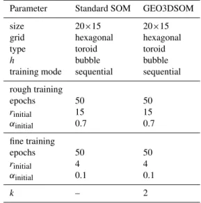
Table 2.Parameters of SOM and GEO3DSOM-analysis.
Parameter Standard SOM GEO3DSOM
size 20×15 20×15
grid hexagonal hexagonal
type toroid toroid
h bubble bubble
training mode sequential sequential
rough training
epochs 50 50
rinitial 15 15
αinitial 0.7 0.7
fine training
epochs 50 50
rinitial 4 4
αinitial 0.1 0.1
k – 2
Figures 3 and 4 show respectively the results of the stan-dard SOM-analysis and the GEO3DSOM-analysis. The U-matrices show the Euclidean distances between the ref-erence vectors of the units by means of a gray scale (black: large distance, white: small distance). The units of the U-matrices are labeled with the cluster number of the sample assigned to the unit, according to Table 1.
Visual inspection of the U-matrices shows that both SOM-analysis are able to extract the clusters from the data. In the U-matrix of standard SOM-analysis a clear separation between groups is only visible between the clusters with D=1 and the clusters withD=0. Although the samples are grouped according to the pre-defined groups, no distinct bor-ders between these groups are present. The U-matrix of the GEO3DSOM-analysis on the other hand, clearly shows that each cluster is separated from another one by a zone of high Euclidian distance between reference vectors.
The accompanying component planes can be used to ex-plore the differences between the clusters. From both Figs. 3 and 4 it can be seen that the area with the samples of cluster 4
Table 3.Quality measures for the theoretical data set.
Quality measure standard SOM GEO3DSOM
qe 0.115 0.145
te 0.128 0.070
ge 0.100 0.097
assigned to it, is characterized byX>0.55,Y >0.55,Z<0.55 andD=1.
In order to asses the quality of the SOM-analysis in repre-senting the data set, three quality measures can be computed; the quantization error (qe), the topographic error (t e) and the geographic error (ge). The quantization error measures the resolution of the SOM and is calculated as the average Eu-clidian distance between an input vector and the reference vector of its best matching unit (Kohonen, 1995). The to-pographic error quantifies the preservation of the topology of the data by calculating the proportion of all data vectors for which first and second best matching unit are not adja-cent units (Kohonen, 1995). Finally, the geographic error is a measure for the ability of the SOM to represent the geo-graphic distribution of the data samples. It is calculated as the geographic distance, the Euclidean distance calculated based on theX,Y andZcoordinates, between an input vector and its best matching unit. Table 3 summarizes the quality mea-sures for the standard SOM-analysis and the GEO3DSOM-analysis.
The quantization error for the standard SOM is lower than for the GEO3DSOM, meaning that the representation of samples is better in the standard SOM. The GEO3DSOM, on the other hand, scores better in terms of topographic and geo-graphic error. The representation of data by the GEO3DSOM is thus better capable of capturing the topology of the data and the geographic information included in the data. 3.2 Hydrochemical data set
The hydrochemical data set is obtained from a monitoring network of the Flemish Government in two regional, sandy, phreatic aquifers, made available through Databank Onder-grond Vlaanderen (DOV, 2006). The data set consists of 47 observation wells, each equipped with three well screens at different depths, resulting in a data set of 131 samples. Fa-cilities in the monitoring well are designed to allow indepen-dent sampling of discrete depth intervals without mixing of groundwater of different depths.
<
Pliocene Miocene (Diest) Early Miocene
Oligocene
Early Oligocene (St. Huijbrechts Hern)
Late Eocene
Middle Eocene (Brussels) Early Eocene
Paleocene
Cretaceous Observation well
0 10 20 30
Belgium
Fig. 5.Study area (after DOV, 2006).
Locally the Brussels sands are overlain by the younger sandy formations of Lede (Middle Eocene) and St. Huibrechts Hern (Early Oligocene). Both aquifers are covered with Quater-nary eolian deposits consisting mainly of sands in the north and loam in the south.
Figure 5 shows the geological map of the study area and location of piezometers used in this study.
A sampling campaign was carried out in the spring of 2005 and from the 20 measured variables, a subset of 12 variables are considered in this analysis. Geographic coordinates, X, Y and the Z position above sealevel of the filter of each sample are included in the data set.
Histograms of the variables (Fig. 6) show that most of the variables are not normally distributed, but rather have a bi-modal (Ca2+ , pH and HCO−3), skewed (e.g. K+, Mg2+, O2and NO−3) or even a lognormal distribution (Fe2+/3+and
Mn2+). In order to avoid bias in the normalization or to make assumptions regarding the distribution of the variables, all parameters, including X, Y, Z are rescaled to a[0,1] inter-val, according to:
xnew=
xold−min(X)
max(X)−min(X) (4)
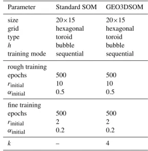
A standard SOM analysis and a GEO3DSOM-analysis are carried out on the normalized data set. The parameters used in both analysis are summarized in Table 4.
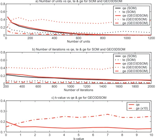
The number of units, the number of iterations and the k-value are determined based on a sensitivity analysis. The re-sults of this sensitivity analysis are rendered in Fig. 7. In the sensitivity analysis only the value of the variable under study is changed, while the other variables are set to the values given in Table 4. The number of grid nodes to be used in a SOM-analysis can be considered as a trade-off between rep-resentation accuracy and generalization accuracy. A small
Table 4.Parameters of SOM and GEO3DSOM-analysis.
Parameter Standard SOM GEO3DSOM
size 20×15 20×15
grid hexagonal hexagonal
type toroid toroid
h bubble bubble
training mode sequential sequential
rough training
epochs 500 500
rinitial 10 10
αinitial 0.5 0.5
fine training
epochs 500 500
rinitial 2 2
αinitial 0.2 0.2
k – 4
0 10 20 0
20 40 60
20 30 40
4 6 8
0 10
2(mg/l) (mg/l)
pH
NO
3
-(mg/l) O
0 50
0 10 20 30
Na+
0 50 100
0 5 10 15 20
K+(mg/l)
0 20 40
0 10 20 30
Mg2+(mg/l)
0 100 200
0 10 20 30
Ca2+(mg/l)
0 50 100
0 50 100 150
Fe2+/3+(mg/l)
0 1 2
0 20 40 60
Mn2+(mg/l)
0 50 100
0 10 20 30
Cl-(mg/l)
0 100 200
0 10 20 30
SO
4
2-(mg/l)
0 500 1000
0 10 20 30 40
HCO
3
-(mg/l)
0 100 200
0 20 40 60 25
Fig. 6.Histograms of the hydrochemical data set.
Table 5.Quality measures for the hydrochemical data set.
Quality measure standard SOM GEO3DSOM
qe 0.127 0.139
te 0.076 0.160
ge 0.028 0.024
and quantization error was found for the 20 by 15 nodes con-figuration (300 nodes). Figure 7b shows the influence of the number of iterations on the quantization, topologic and ge-ographic error. The number of iterations shown are the to-tal number of iterations after rough and fine training. After 1000 iterations (500 rough training and 500 fine training) the topologic and geographic error are stabilized, while the quan-tization error only decreases slightly. The sensitivity analysis with regards to the k-value (Fig. 7c) reveals that with increas-ing k-value, the geographic error increases rapidly and the quantization error decreases. Once again a compromise has to be found between the weight given to the geographic co-ordinates and the overall quantization. After visual examina-tion of the ability of the different maps to represent the data, a k-value of 4 produced the best results both with respect to low quantization and geographic error and with respect to vi-sualizing and grouping of the data. The choice of 4 for the geographic tolerancekimplies that the search of the BMU
is restricted to the units lying within a radius of 4 units sur-rounding the geographically closest unit.
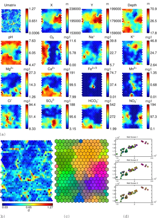
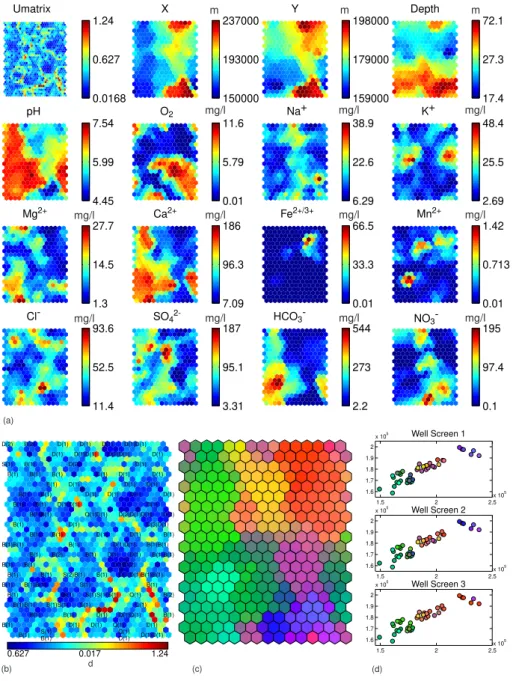
The results of both analysis are depicted in Fig. 8 (stan-dard SOM) and Fig. 9 (GEO3DSOM). The visualized results are (a) component planes, (b) U-matrix labeled with geol-ogy (B: Brussel sands, S: St. Huybrechts Hern sands, D: Di-est sands, Q: Quaternary deposits), (c) false coloring of the SOM based on the U-matrix and finally (d) spatial distribu-tion well screens, colored using the false coloring. The spa-tial distribution of the groups is organized per well screen, with screen 1 being the shallowest screen and screen 3 the deepest. The false coloring of the units of the self-organizing map is carried out in such a way that units with similar weight vectors have similar colors, using a naive contraction model based on the U-matrix according to the algorithm proposed by Himberg (2000). The resulting color coding is then ap-plied to the representation of the well screens. In this way a fuzzy ordering of the well screens is carried out, linking them through the false colored SOM with the component planes, without having to manually delineate groups.
0 200 400 600 800 1000 1200 0
0.2 0.4 0.6 0.8
qe (SOM) te (SOM) qe (GEO3DSOM) te (GEO3DSOM) ge (GEO3DSOM)
200 400 600 800 1000 1200 1400 1600 1800 2000 0
0.2 0.4 0.6 0.8
Number of iterations
qe (SOM) te (SOM) qe (GEO3DSOM) te (GEO3DSOM) ge (GEO3DSOM)
0 1 2 3 4 5 6 7 8 9 10
0.1 0.2 0.3 0.4
c) k-value vs qe & ge for GEO3DSOM
k-value
qe ge (x10) a) Number of units vs qe, te & ge for SOM and GEO3DSOM
Number of units
b) Number of iterations vs qe, te & ge for SOM and GEO3DSOM
Fig. 7. Results of the sensitivity analysis with respect to(a)the number of units,(b)the number of iterations and(c)the value of the
geographical tolerancekfor SOM and GEO3DSOM.
noticeable on the component planes (Fig. 8a and Fig. 9a), where distributions of the variables on the component planes of the standard SOM are rather smooth compared to those of the GEO3DSOM. This is mainly due to the better topological representation of the standard SOM.
The geographic error of the GEO3DSOM, however, is 15% smaller than in the standard SOM, implying that the geographic representation of the GEO3DSOM resembles the data set more closely.
On the U-matrices (Figs. 8b and 9b), it is also noticeable that the U-matrix of the GEO3DSOM divides the SOM in a large number of well separated groups, while the number of groups in the standard SOM is smaller and the borders between groups are less distinct. The more distinct borders between groups in the GEO3DSOM U-matrix results in a higher resolution for the false coloring compared to the stan-dard SOM coloring (Figs. 8c and 9c).
Both SOM-variants succeed in distinguishing between samples originating from the Diest and the Brussels aquifers, as can be deduced from the geology-labeled U-matrices (Figs. 8b and 9b). The component planes reveal that pH and concentrations of calcium and bicarbonate are relatively high in the Brussels aquifer. This difference is due to the presence of calcite in the Brussels sands, while calcite is almost absent
in the Diest sands (Laga et al., 2001; Lagrou et al., 2004). In the false coloring of the GEO3DSOM this geology related subdivision is clearly visible through a distinct difference in coloring. In the coloring of the SOM however the distinc-tion between Diest and Brussels samples is, if present, only noticeable through subtle color differences.
The Quaternary samples can also be differentiated from the rest, albeit less clear, since the Quaternary samples are characterized by an overall very low mineralization, with the exception of nitrate and chloride which can be locally very high. Since these well screens are rather shallow and the Quaternary deposits consist of sands and gravels, the com-position of groundwater is very close to the comcom-position of rain water, hence the low pH, and very susceptible to an-thropogenic influences like chlorine and nitrate contamina-tion. In both SOM variants the region with Quaternary sam-ples is apparent from the false coloring. A smaller varia-tion in groundwater chemistry can be detected in the Brus-sels aquifer, where the most northern and the north eastern samples are characterized by lower Mg2+concentrations. In the coloring of the SOMs this is noticeable through subtle difference in shades of green.
(a)
(b) (c) (d)
1.5 2 2.5
x 105 1.6
1.7 1.8 1.9 2
x 105 Well Screen 1
1.5 2 2.5
x 105 1.6
1.7 1.8 1.9 2
x 105 Well Screen 2
1.5 2 2.5
x 105 1.6
1.7 1.8 1.9 2
x 105 Well Screen 3 0.0306 0.651 1.27 Umatrix 153000 195000 238000 X 159000 179000 199000 Y 17.8 26.5 70.9 Depth 4.47 6.05 7.63 pH 0.00 5.78 11.6 O2 5.7 22.7 39.8 Na+ 2.64 24.7 46.8 K+ 1.26 14.3 27.3 Mg2+ 7.99 99.5 191 Ca2+ 0.01 37.4 74.7 Fe2+/3 0.01 0.68 1.35 Mn2+ 8.33 51.4 94.4 Cl-3.15 95.6 188 SO4 2-1.99 272 542 HCO3 -0.1 97.3 194 NO3-
mg/l mg/l mg/l
mg/l mg/l mg/l
mg/l mg/l mg/l
mg/l mg/l
m m m
0.03 0.65 1.27 D(2) D(1) Q(1) D(1) S(1) B(1) B(1) B(2) B(1) B(2) D(1) D(1) D(1) D(1) B(1) B(1) B(1) B(1) D(1) D(1) S(1) S(1) B(1) B(1) B(1) B(2) B(1) D(1) D(1) D(1) B(1) B(1) S(1) B(1) D(1) D(1) D(1) S(1) B(1) S(1) B(1) S(1) S(1) D(1) D(1) D(1) B(1) S(1) B(1) S(2) D(1) D(2) B(1) B(1) B(1) B(1) D(1) D(2) D(1) D(1) D(1) B(1) B(1) D(3) D(2) D(2) D(1) B(1) B(1) B(1) B(1) B(1) D(1) D(1) D(1) D(1) Q(1) B(1) B(1) D(1) D(2) D(3) B(1) B(1) B(2) Q(2) D(1) D(1) D(1) B(1) B(1) B(1) B(1) D(1) D(2) D(1) B(1) B(1) D(2) Q(2) D(1) D(1) B(1) B(2) B(2) D(1) Q(1) D(1) D(2) d
Fig. 8.Results of the SOM-analysis of the hydrochemical data
set.
(a)U-matrix and component planes
(b)labeled U-matrix
(c)false coloring of U-matrix
(d)spatial distribution of well screens, using false coloring.
both aquifers there are zones with low oxygen concentra-tions and elevated iron and manganese. These groups consist of the deeper samples (Figs. 8d and 9d) and nitrate concen-trations are on average lower in these groups. Due to the ubiquitous presence of iron and manganese bearing minerals like glauconite and iron-oxides in the Diest aquifer (Lagrou et al., 2004), the iron concentrations are rather high in the
Diest aquifer when oxygen concentrations are low. This sub-division of the data is determining the color coding of the standard SOM, while in the GEO3DSOM this feature is sub-ordinate to the coloring based on pH, Ca2+and HCO−3.
0.0168 0.627 1.24 Umatrix 150000 193000 237000 X 159000 179000 198000 Y 17.4 27.3 72.1 Depth 4.45 5.99 7.54 pH 0.01 5.79 11.6 O2 6.29 22.6 38.9 Na+ 2.69 25.5 48.4 K+ 1.3 14.5 27.7 Mg2+ 7.09 96.3 186 Ca2+ 0.01 33.3 66.5 Fe2+/3+ 0.01 0.713 1.42 Mn2+ 11.4 52.5 93.6 Cl-3.31 95.1 187 SO4 2-2.2 273 544 HCO3 -0.1 97.4 195 NO3
-mg/l mg/l mg/l
mg/l mg/l mg/l
mg/l mg/l mg/l
mg/l mg/l
m m m
0.017 0.627 1.24 D(2) S(1) B(1) B(1) B(1) B(1) B(1) B(1) B(1) B(1) B(1) B(1) B(1) B(1) B(1) B(2) B(1) B(1) B(1) B(1) B(1) B(1) B(1) B(1) B(1) B(1) B(1) B(1) B(1) B(1) S(1) B(1) D(1) B(1) B(1) B(1) B(2) B(1) D(1) D(1) S(2) S(1) S(1) B(1) D(1) D(2) D(1) D(1) D(1) B(1) B(1) D(1) D(1) D(1) D(1) Q(1) B(1) S(1) S(1) S(1) D(1) D(1) D(1) B(1) S(1) D(1) D(1) D(1) D(2) D(1) D(1) S(1) D(1) D(1) D(2) D(1) D(1) D(1) Q(1) Q(1) Q(1) D(1) D(1) D(1) D(1) D(1) D(1) D(1) D(1) D(2) D(1) Q(1) Q(1) D(1) D(1) D(1) B(1) Q(1) D(1) D(1) D(1) D(1) D(1) D(3) B(1) B(1) B(1) B(1) D(1) D(1) D(1) D(3) D(1) B(1) B(1) B(1) B(2) B(1) d (a) (b)
1.5 2 2.5
x 105 1.6
1.7 1.8 1.9 2
x 105 Well Screen 1
1.5 2 2.5
x 105 1.6
1.7 1.8 1.9 2
x 105 Well Screen 2
1.5 2 2.5
x 105 1.6
1.7 1.8 1.9 2
x 105 Well Screen 3
(c) (d)
Fig. 9.Results of the GEO3DSOM-analysis of the hydrochemical data set.
(a)U-matrix and component planes
(b)labeled U-matrix
(c)false coloring of U-matrix
(d)spatial distribution of well screens, using false coloring.
Both SOM-variants succeed in isolating and identifying these outlying values.
4 Conclusions
The self-organizing map algorithm has proved to be a very valuable tool in the visualization and interpretation of large, multivariate data sets.
To incorporate spatial information in a self-organizing map analysis, GEO3DSOM is developed and its performance in clustering of both an artificial and a real life data set is compared to the standard SOM.
exploratory data analysis in order to capture relationships be-tween variables and the structure of data.
The GEO3DSOM on the other hand outperforms the stan-dard SOM in providing a grouping of the data in a spatially coherent way. Analysis of both the artificial and the real life data sets showed that the GEO3DSOM is capable of a more detailed grouping of both regularly and irregularly dis-tributed spatial data, compared to the standard SOM with geographical coordinates included in the data set. As is to be expected, the information about the data set at hand obtained through the component planes and the U-matrices by both versions of the SOM is very similar. The pseudo-coloring applied to both variants of the SOM-algorithm how-ever shows some clear differences between both techniques. The explicit incorporation of the geographic coordinates in the GEO3DSOM algorithm results in greater differences between groups in the U-matrix. This results in an in-creased resolution in the pseudo-coloring of the units. In the GEO3DSOM both the geology related subdivision and the vertical subdivision is apparent from the coloring, while in the standard SOM the coloring is dominated only by the vertical subdivision based on oxygen, iron and manganese. Within the samples having elevated oxygen and nitrate con-centrations, a subtle differentiation between Brussels and Di-est samples can be seen, while this differentiation is com-pletely absent in the group of samples with low oxygen and nitrate concentrations. Both coloring schemes do however identify the presence of outliers in the Brussels sands aquifer. In conclusion it can be stated that both techniques succeed very well in providing more insight in the quality data set, highlighting the main differences and pointing out anoma-lous wells. Incorporation the spatial correlation through in-cluding the geographic coordinates in the BMU-selection procedure of GEO3DSOM, however, provides the advantage of an increased resolution, while still maintaining a general-ization of the data set.
Acknowledgements. The authors wish to thank AMINAL for providing data through their website (DOV, 2006).
Edited by: D. Solomatine
References
Alvisi, S., Mascellani, G., Franchini, M., and Bardossy, A.: Water level forecasting through fuzzy logic and artificial neural network approaches, Hydrol. Earth Syst. Sci. 10, 1–17, 2006.
ASCE Task Committee on Application of Artificial Neural Net-works in Hydrology: Artificial neural netNet-works in hydrology. II: Hydrologic applications, J. Hydrol. Eng., 5(2), 124–137, 2000. Bac¸˜ao, F., Lobo, V., and Painho, M.: The self-organizing map, the
Geo-SOM, and relevant variants for geosciences, Computers and Geosciences, 31(2), 155–163, 2005a.
Bac¸˜ao, F., Lobo, V., and Painho, M.: Self-organizing maps as sub-stitute for K-means clustering, in: International conference on
computational science, edited by: Sunderarm, V. S., van Al-bada, G., Sloot, P., and Dongarra, J. J., International conference on computational science 2005, Lecture Notes in Computer Sci-ence, Springer-Verlag Berlin, Berlin, 3516, 476–483, 2005b. Chang, H. C., Kopaska-Merkel, D. C., and Chen H. C.:
Identifica-tion of lithofacies using Kohonen self-organizing maps, Comput-ers and Geosciences, 28(2), 223–229, 2002.
Coppola, E., Szidarovsky, F., Poulton, M., and Charles, E.: Artifi-cial neural network approach for predicting transient water lev-els in a multilayered groundwater system under variable state, pumping and climate conditions, J. Hydrol. Eng., 8(6), 348–360. 2003.
Davis, J. C.: Statistics and data analysis in geology, John Wiley & Sons, Inc, New York, 1986.
Databank Ondergrond Vlaanderen: http://dov.vlaanderen.be, 2006. G¨uler, C., Thyne, G. D., and McCray, J. E.: Evaluation of graphi-cal and multivariate statistigraphi-cal methods for classification of water chemistry data, Hydrogeology J., 10(4), 455–474, 2002. Himberg, J.: A SOM Based Cluster Visualization and Its
Applica-tion for False Coloring, Proceedings of InternaApplica-tional Joint Con-ference on Neural Networks (IJCNN2000), 3, 587–592, 2000. Hong, Y. S. and Rosen, M. R.: Intelligent characterisation and
di-agnosis of the groundwater quality in an urban fractured-rock aquifer using an artificial neural network, Urban Water, 3(3), 193–204, 2001.
Jain, A. K., Mao, J., and Mohiuddin, K.: Artificial Neural Net-works: a tutorial, IEEE Computer, 26(3), 31–44, 1996.
Kaski, S.: Data exploration using Self-Organizing Maps, Acta Poly-technica Scandinavica: Mathematics, computing and manage-ment in engineering, Series No 82, 57, 1997.
Kohonen, T.: Self-organizing maps. Springer, Berlin, 1995. Koua, E. L., Maceachren, A., and Kraak, M.-J.: Evaluating the
us-ability of visualization methods in an exploratory geovisualiza-tion environment, Int. J. Geographical Informageovisualiza-tion Sci., 20(4), 425-448, 2006.
Lacassie, J. P., Roser, B., Ruiz del Solar, J., and Herve, F.: Dis-covering geochemical patterns using self-organizing neural net-works: a new perspective for sedimentary provenance analysis, Sedimentary Geology, 165(1–2), 175–191, 2004.
Laga, P., Louwye, S., and Geets, S.: Paleogene and Neogene lithos-tratigraphic units (Belgium), Geologica Belgica, 4(1–2), 135– 152, 2001.
Lagrou, D., Dreesen, R., and Broothaers, L.: Comparative quanti-tative petrographical analysis of Cenozoic aquifer sands in Flan-ders (N Belgium): overall trends and quality assessment, Mate-rials Characterization, 53, 317–326, 2004.
Lambrakis, N., Antonakos, A., and Panagopoulos, G.: The use of multicomponent statistical analysis in hydrogeological environ-mental research, Water Res., 38(7), 1862–1872, 2004.
Lischeid, G.: Taming awfully large data sets: using self- organizing maps for analyzing spatial and temporal trends of water quality data, Geophys. Res. Abstr., 5, 01879, 2003.
Love, D., Hallbauer, D., Amos, A., and Hranova, R.: Factor anal-ysis as a tool in groundwater quality management: two southern African case studies, Phys. Chem. Earth, 29(15–18), 1135–1143, 2004.
348–354, 2005.
Mingoti, S. A. and Lima, J. O.: Comparing SOM neural network with Fuzzy c-means, K-means and traditional hierarchical clus-tering algorithms, European J. Operational Res., 174, 1742– 1759, 2006.
Ozerdem, M. S., Ustundag, B., and Demirer, R. M.: Self-organized maps based neural networks for detection of possible earthquake precursory electric field patterns, Advances in Engineering Soft-ware, 37(4), 207–217, 2006.
Openshaw, S. and Turton, I.: A parallel Kohonen algorithm for the classification of large spatial datasets, Computers and Geo-sciences, 22(9), 1019–1026, 1996.
Penn, B. S.: Using self-organizing maps to visualize
high-dimensional data, Computers and Geosciences, 31(5), 531–544, 2005.
Poulton, M. M., Sternberg, B. K., and Glass, C. E.: Location of sub-surface targets in geophysical data using neural networks, Geo-phys., 57(12), (1534–1544), 1992.
Richardson, A. J., Risien, C., and Shillington, F. A.: Using self-organizing maps to identify patterns in satellite imagery, Progress in Oceanography, 59(2-3), 223–239, 2003.
Sanchez-Martos, F., Aguilera, P. A., Garrido-Frenich, A., Torres, J. A., and Pulido-Bosch, A.: Assessment of groundwater quality by means of self-organizing maps: application in a semi-arid area, Environ. Manage., 30(5), 716–726, 2002.
Skupin, A. and Hagelman, R.: Attribute space visualization of demographic change, Eleventh ACM international symposium on Advances in geographic information systems, New Orleans, Louisiana, USA, 2003.
Takatsuka, M.: An application of the self-organizing map and inter-active 3-D visualisation to geospatial data, GeoComputation’01 (6th International Conference on GeoComputation, Brisbane, Australia, 2001.
Ultsch, A. and Herrmann, L.: The architecture of emergent self-organizing maps to reduce projection errors, in: ESANN2005 13th European Symposium on Artificial Neural Networks, Bruges, Belgium, 1–6, 2005.