Núcleo de Investigação em Microeconomia Aplicada
Universidade do Minho
An experimental analysis of
grandfathering vs dynamic
auctioning in the EU ETS
Anabela Botelho
Eduarda Fernandes
Lígia Pinto
October2010
Working Paper Series
No. 39/2010
An experimental analysis of grandfathering vs dynamic auctioning in the EU ETS by
Anabela Botelho, Eduarda Fernandes, Lígia Costa Pinto* October 2010
Abstract
This study constitutes a first attempt to experimentally test the performance of a 100% auction versus a 100% free allocation of CO2 permits under the rules and parameters that mimic the EU ETS (imperfect competition, uncertainty in emissions’ control, and allowing banking). It also incorporates a first attempt to include in the analysis measures of the risk preferences of subjects participating in emission permits experiments. Another distinctive feature of this study is the implementation of a theoretically appropriate auction format for the primary allocation of emission permits. Our experimental results indicate that the EU ETS has the potential to reduce CO2 emissions, achieving targets considerably more restrictive than the current ones at high efficiency levels, both with auctioned and free emission permits. Auctioning, however, reveals a clear potential to do better than grandfathering the initial allocation of permits. In addition, the results reveal that concerns about undue scarcity, and corresponding high prices, in secondary markets generated by a primary auction market are not warranted under the proposed dynamic auction format.
Keywords:
EU ETS, auctioning, grandfathering, banking, Ausubel auctionJEL Classification: Q54, C9
*Department of Economics, University of Minho and NIMA (Botelho and Pinto), and ESTG, Polytechnic Institute of Leiria (Fernandes). We thank the Fundação para a Ciência e Tecnologia for research support under grant POCTI/ECO/45435/02. Corresponding author: Anabela Botelho, Departamento de Economia, Escola de Economia e Gestão, Universidade do Minho, Campus de Gualtar, 4710-057 Braga, Portugal. Tel. +351-253-604538. Fax: +351-253-601380. E-mail: [email protected]
1
1. Introduction
The use of auctions as a rule for the initial allocation of CO2 emission permits in the next stages of the EU ETS (European Union Emissions Trading Scheme) is a subject that the European Commission and its Member-States are currently discussing and evaluating. This paper is the first to experimentally test the Ausubel (2004) auction for the case of CO2 emission permits in the EU ETS.
The European Union has stepped forward in its commitment for GHG (greenhouse gases) emissions’ reduction by defining on its Climate Policy the goal to reduce GHG at least 20% by 2020 compared with 1990 levels. The EU ETS is therefore a major policy initiative to achieve CO2 emissions’ reductions. This political choice to fight a global negative externality is on the same line as the Kyoto Protocol flexible mechanisms, which included an international market for GHG transaction, as well as the more recent RGGI – Regional Greenhouse Gas Initiative, for ten states of the US.1
Emission permit markets have been used for local pollutants like SO2 (sulphur dioxide) since the 80s and 90s, mainly in the US and Canada, but its application for a global pollutant, like CO2, has an innovative character. It is for this reason, and because the EU ETS dimension and complexity is considerably different from previous markets (due to its multi-jurisdictional political structure, connection between differing domestic emissions permits programs, etc.), that we focus on this specific application of emission permits markets (EPM).
Several studies exist about the EU ETS and a consensual point is usually highlighted: the importance of the institutional rules adopted for its performance, as for any other EPM. Particularly, the initial allocation rule decided under the 2003/87/EC Directive (grandfathering) recurrently appears as one of the least positive aspects of the institution chosen to implement the EU ETS. In fact, auctioning instead of grandfathering is presently recommended inside the EU for the third phase of the market (starting 2013), as we can find in the COM(2008) 16 final from 23.1.2008, pp.7:
“Auctioning best ensures efficiency of the ETS, transparency and simplicity of the system and avoids undesirable distributional effects. Auctioning also
1 Connecticut, Delaware, Maine, Maryland, Massachusetts, New Hampshire, New Jersey, New York,
2
best complies with the polluter-pays principle and rewards early action to reduce emissions. For these reasons auctioning should be the basic principle for allocation.”
Neuhoff and Matthes (2008) summarize the main reasons why auctioning should be adopted for the initial allocation of CO2 emission permits in the EU ETS as follows:
i) it eliminates uncertainties about future changes in the allocation schemes, favoring
investment decisions and innovation from firms included in the 2003/87/EC Directive;
ii) it allows governments to receive the necessary revenue to encourage innovation, to
reduce taxes, or to compensate the poorest families from increases in energy prices as a consequence of the environmental policies; iii) it is a simple and fair scheme to allocate emission permits, which guarantees a higher public support. In fact, as we read in the Commission Recommendation above, instead of the Coasian “right to pollute” it is the Pigouvian “polluter-pays” principle that is applied with auctioning, which might bring a higher consensus around the more restrictive environmental policies the EU is about to impose in the next years.
Our study contributes to the ongoing debate concerning the use of auctions as a rule for the initial allocation of CO2 emission permits in the next stages of the EU ETS. Under Dales (1968) and Montgomery (1972) original models for EPM, the initial allocation rule does not affect the efficiency of the policy instrument (it matters only on equity terms). Our investigation examines whether this is the case for the EU ETS. We therefore experimentally investigate the performance of an EPM similar to the EU ETS under alternative allocation rules: grandfathering and auctioning.
The experimental methodology has been widely used in studies examining emission permit markets in the US and Canada with purposes similar to ours: works by Godby et al. (1997), Cronshaw and Brown-Kruse (1999), Franciosi et al. (1999), Cason
et al. (1999), Mestelman et al. (1999) and Gangadharan et al. (2005) are just a few.
Surprisingly, this is not the case for the EU ETS. To our knowledge, this is the first experimental study to include both the rules and the parameters that parallels the EU
3
ETS structure.2 Our experimental market is characterized by imperfect competition (few agents with different dimensions, different marginal abatement costs and different environmental targets) under a cap-and-trade system, with banking allowed, a secondary market represented by a double auction with discriminative prices and a penalty structure for noncompliance similar to the 2003/87/EC Directive.
Another novel feature of our experimental design is the implementation of the Ausubel (2004) auction as the rule for the initial allocation of CO2 emission permits. Although several types of auctions have already been experimentally tested for the initial allocation of emission permits, the present study is the first to implement a dynamic auction for the multi-unit demands that characterize this market, and that, theoretically, yields the same results as the Vickrey auction, its static counterpart.
In addition, we included the elicitation of subjects’ risk preferences in our experimental design. This is, therefore, the first study on EPM that explicitly classifies participants in the experiment with respect to their attitudes towards risk, allowing us to test the hypothesis raised in the literature concerning the relationship between subjects’ banking behavior and their attitudes towards risk.
Below we develop our experimental design, and subsequently we discuss the structural features (parameters) implemented in our experiments. Then we detail experimental procedures, and in section 5 present our working hypotheses. Results are reported in section 6, and the last section concludes.
2. Experimental design
Our experimental variable is the rule for the initial allocation of CO2 emission permits in the EU ETS. Hence, two experimental treatments were conducted differing only with respect to the initial allocation rule: grandfathering vs. auctioning.
2 For example, Benz and Ehrhart (2007) experimental study on the initial allocation of CO
2 allowances in
the EU ETS is far from implementing its institutional features and therefore does not constitute a testbed for this market.
4
All our experimental sessions were computerized (using the zTree software from Fischbacher (2007)) and had three parts: 1) A standard socio-demographic questionnaire; 2) The implementation of a Multiple Price List (MPL) for the elicitation of subjects’ risk attitudes; and, 3) An Emission Permits Market (EPM). The first two parts were included for control purposes, and the last and central part of the experimental sessions implements the market for CO2 emission permits under the features of the EU ETS. Each of these parts was initiated only when all participants finished all the tasks in the previous part.
A. Elicitation of risk attitudes
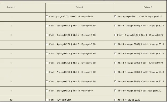
Elicitation of subjects’ risk attitudes was carried out using the instrument developed by Holt and Laury (2002). This instrument, a Multiple Price List (MPL), entails presenting subjects a set of ordered binary lotteries to choose all together. In our implementation of the MPL design, subjects were required to make a series of 10 choices between two payment options (or lotteries), A or B. Each of these payment options comprised a high prize and a low prize. The high prize for payment option A was €2.00 and the low prize €1.60; the high and low prizes for payment option B were €3.85 and €0.10, respectively. Each subject received the high or the low prize of the chosen payment option according to the number of a ball randomly extracted from a bag containing 10 balls individually numbered from 1 to 10.
Figure 1 shows the MPL presented to subjects in each of our experimental sessions (translated from Portuguese). The first row in this table reveals that the probability of getting the high prize in each of the payment options is 1/10 so that only extremely risk loving subjects are expected to pick payment option B in the first decision. The probabilities associated with the high prize in each option increase by 10 percentage points as subjects proceed down the table, and the last row pays the high prize in each option for sure. The expected values associated with each decision and payment option indicate that a risk-neutral subject is expected to choose option A in the first four decisions, and switch to option B thereafter. Only highly risk averse subjects are expected to choose option A in the second last row, but even those are expected to switch to option B in the last decision.
5
Following Holt and Laury (2002), subjects were free to choose between these two payment options but in our experiments we imposed the consistency restriction that after choosing option B at any one decision row subjects were not allowed to switch back to option A, thereby avoiding the erratic choices problem and consequent difficulties associated with its analysis. Subjects were also informed that earnings from this part of the experiment were to be determined at the end of the session using the following procedure: each subject extracts one ball from the bag with 10 balls to determine which of the 10 decisions is to be used for payout for that subject, and another random draw determines whether the subject receives the high or low prize according to the chosen payment option in that decision. This random lottery incentive procedure is commonly applied with the MPL instrument, and its properties are thoroughly discussed by Harrison and Rutström (2008).
The data collected from this part of the experiment allow us to classify subjects as risk averse, risk neutral or risk loving in order to verify whether their banking behavior in the third part of the experiment can be explained in terms of subjects’ risk attitudes.
6
B. Market Institution
A sequence of 10 market periods constituted the third part of every experimental session. The implemented market institution resembles as close as possible the rules predicted on the 2003/87/EC Directive for the EU ETS. To examine the effects of the rule for the initial allocation of CO2 emission permits in the EU ETS, two treatments were implemented: one treatment with grandfathering as in the 2003/87/EC Directive, and another treatment with auctioning of all the available emission permits, following the recommendations in COM(2008) 16 final from 23.1.2008. All language in the experimental instructions was context-free. Emission permits, environmental goals or policy instruments for regulation were never mentioned. Subjects were told they were placed in a market where each firm (subject) must surrender a certain number of units of an abstract good in each period. Each unit had a certain cost known only to the subject, and earnings could be realized through trading in the market under pre-specified rules.
In the grandfathering treatment, participants knew how many units they would be given in the session (emission permits): a fixed amount, equal in every period. In the example shown in Figure 2, the subject must a priori surrender 6 (activity) units in every period, each at the indicated cost in experimental points, and the units given are marked with a “Yes” (ie, the subject does not bear the costs of the units that are given), amounting four given units in each period for a total of 40 given units in the session. The subjects’ first decision in each period was either to use all the allocated permits for the period or to save some of them for the future, ie, a banking decision. This feature of the design means that, concerning the intertemporal validity of emission permits, we allowed banking but not borrowing, as established in the 2003/87/EC Directive: non-used permits are still valuable for the following periods but market participants are not allowed to use in the current period emission permits they know will be given to them in the next periods.3 Subjects entered their decisions in the spaces provided under “Planned Use”. Thus, if the subject in the first period decided to save one permit for use in the second period, he would enter a “3” in the provided space for the first period and
3 Borrowing is not explicitly allowed in the EU ETS. However, because of the gap between the delivery
date of emission permits from one year (30th April of the following year) and the allocation of emission permits for the next one, firms might in fact borrow emission permits.
7
a “5” in the provided space for the second period. Subjects were free to use all the allocated permits in the current period or to save some or all of them for use in future periods as long as the planned use in each period did not exceed the total number of units the subject must surrender in each period, and the planned use over the 10 periods is equal to the total number of allocated permits in the session (restrictions and appropriate error messages were programmed in the zTree software to ensure compliance with these rules).
Figure 2 – zTree screen for banking decision
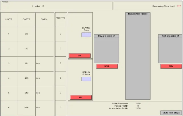
Once all subjects were done with their banking decision, a new zTree screen opened the market for emission permits transactions. For this (secondary) market, a double auction with discriminative prices was implemented. Figure 3 illustrates the zTree screen for one subject during this stage. The number of units the subject must surrender in the period, their respective costs, and the number of permits he is using in the current period (according to the banking decision in the previous stage) is shown in
8
the table at the left hand side of the screen. Subjects make profits by buying non-given units at a price lower than their cost, and by selling given units at a price higher than their cost.
Subjects submit bids in the space provided under “Buying Price”, and offers in the space provided under “Selling Price”. They were free to change their bids and offers at any time under the constraints that only improving bids and offers were allowed. In addition to obey the improvement rule while making their bids/asks, only profitable transactions were allowed in this market. Moreover, no re-sale was possible in the market (once bought, emission permits had to be used to avoid abatement costs). Standing bids were shown in the box under “Buy at a price of” and any seller could accept a standing bid at any time by clicking the button “Sell”. Standing offers were shown in the box under “Sell at a price of” and any buyer could accept a standing offer at any time by clicking the button “Buy”. Once a unit was bought or sold, it appeared appropriately marked as such under the column “Given” and the associated profits under the column “Profits”.
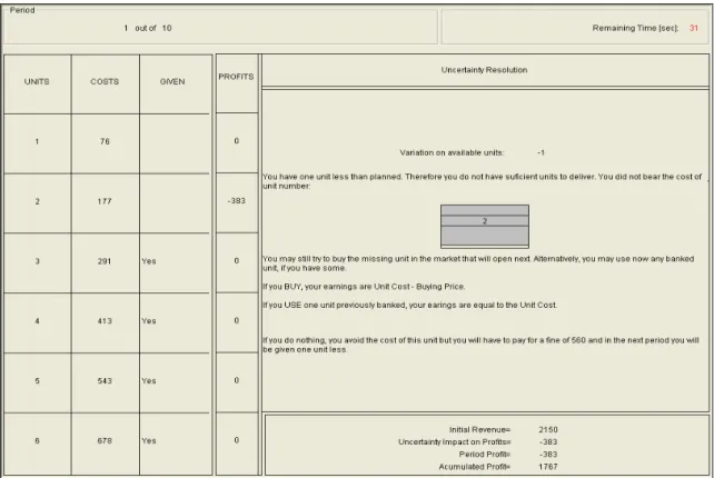
Subjects knew only their own marginal abatement costs and maximum permits needed, but each transaction made in the market was publicly known (although the seller/buyer identification was not available) as shown in the box under “Transaction Prices”. This market closed when time limit was reached (3 minutes) or all participants pressed the “OK to next stage” button on the zTree screen. After that, subjects were prompted to an “uncertainty resolution” screen as illustrated in Figure 4.
9
Figure 3 – zTree screen for the initial market
Uncertainty in the control of emissions was introduced in the experiment following the procedure devised by Godby et al. (1997), ie, a random variation on emissions was drawn from a uniform distribution over the values (-1, 0, +1) where a “-1” means the subject had to surrender one more unit than initially predicted, a “+“-1” means the subject supported the cost of one more unit than necessary, and a “0” means that the number of units the subject had to surrender was exactly the initially predicted number.
To ensure comparability of results, we used the same distribution for the different experimental sessions. Subjects with a unit deficit or surplus were reminded of the possible courses of action and their consequences in each and every period, as Figure 4 illustrates. Subjects with a unit surplus could save it for future use, or could try to sell it in a reconciliation market. Subjects with a unit deficit could use any previously saved unit (in the banking phase) to clear it at this moment, or could try to buy one more unit in the reconciliation market. In case the subject did not opt for any of these options, he would have to pay a fine for noncompliance about four times the emission permits equilibrium price, and, in addition, surrender one more emission permit in the next
10
market period. These rules for noncompliance mimic those included in article 16º of the 2003/87/EC Directive.
Figure 4 – zTree screen for uncertainty resolution
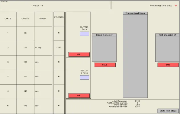
This screen was opened for 40 seconds each period to avoid subjects just bypassing the information. At the end of this time, the screen for the reconciliation market opened for subjects with unit deficit or surplus. Figure 5 illustrates the screen for this market. The rules for this market were similar to the initial market. However, less time was given for the transactions to be concluded (1.5 minutes), only the deficit/ surplus unit could be traded, and non-profitable transactions were allowed.
11
Figure 5 – zTree screen for the reconciliation market
The auctioning treatment was equal to the grandfathering treatment in every respect except that instead of being given for free, emission permits had to be bought in an initial auction where all subjects participated as buyers. Given that auctioning as a rule for initial allocation of permits is not yet a reality for the EU ETS, we first had to decide which auction format to implement. Sealed-bid uniform price auctions are well known by utilities regulated in the EU ETS, have been used in Ireland, Hungary and Lithuania in the first phase of the EU ETS, and Holt et al. (2007) recommend it to auction CO2 under the RGGI – Regional Greenhouse Gas Initiative. However, the literature has shown that this auction format results in allocative inefficiency (Ausubel and Cramton (1998) or Holt (2006), for example) in multi-unit contexts as the one considered here. The second-price sealed bid auction format – the Vickrey auction - is theoretically recognized as the most efficient for multiple-unit auctions. Despite its superiority, this auction format is not usually implemented in practice due to its complexity, and the consequent cognitive difficulties it entails. We therefore decided to implement the ascending-bid auction proposed by Ausubel (2004), a dynamic counterpart to the Vickrey auction that theoretically yields the same results but has the
12
advantages of maintaining the privacy of bidders’ valuations, and is much simpler for them to understand.
Although a number of experimental studies have already examined the performance properties of the Ausubel (2004) dynamic auction (eg. Kagel and Levin (2001), Engelmann and Grimm (2004), and Manelli et al. (2006)), this is, to our knowledge, the first experimental study implementing this auction for the initial allocation of CO2 emission permits within a market characterized by uncertainty, banking, a secondary market and a reconciliation market.
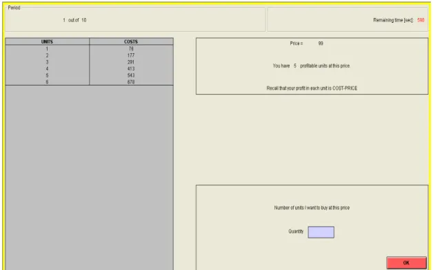
Figure 6 illustrates the zTree screen subjects saw in the auction for the initial allocation of permits. Following the rules proposed by Ausubel (2004), the auctioneer calls a price, and each subject responds with quantities. In the example below, the auctioneer is calling a price of 99 experimental points, and the subject is informed of how many units are profitable at that price, and reminded that earnings in this auction equal the difference between the cost of each unit and the price paid for its acquisition. The subject is then free to respond any number of units, as long as it does not exceed a maximum number of units determined for each subject according to a budget constraint (for each subject, this is the number of activity units times the equilibrium market price divided by the auctioneer’s initial calling price). This process iterates with increasing prices called by the auctioneer until demand is equal or less than total supply, and the auction closes at this point.
It is important to note that the subject’s payment is not equal to the quantity bought in the auction times the closing price. In fact, for each bidder and at each called price, the auctioneer determines whether total demand by the other bidders is less than total supply. If that is the case, then the difference is considered “clinched”, and the newly clinched units are sold to the bidder at the called price; the price paid is therefore the opportunity cost of awarding the unit to the winning bidder. A private value, incomplete information version of the Ausubel (2004) auction was implemented. This means subjects knew only their own marginal abatement costs and while the auction was open, they did not know anything about others demand nor the result from their own proposals at each price. As long as the price in the auction increased, subjects could conclude only that the demand for permits was still higher than supply. When the
13
auction closed, each subject was informed of how many units he was awarded and their respective prices. At this point, the auctioning treatment proceed in the same manner as the grandfathering treatment, with “Given” units now designated “Acquired” units, corresponding to those bought by the subject in this auction.
Figure 6 – zTree screen for the Ausubel auction
A summary of all the sequential phases or stages that constituted each market period in the third part of the experimental sessions is presented in Table 1.
14
Table 1 – Summary of the different stages from the 3rd part of the experimental design Stage 0: Initial Auction for acquisition of emission permits
Possibility of making bids (quantities) at each price proposed by the auctioneer. This stage does not exist in the grandfathering treatment.
Stage 1: Banking decision
Subjects decide whether or not to use all the permits in the current period– i.e., decide to bank or not all or some of their permits for future use.
Stage 2: Permit market
Possibility of buying from or selling permits to other subjects. Emission permits for the current period, not banked on the previous stage, can be sold at a price higher than the marginal abatement cost, and permits may be bought to cover units to abate, at a cost inferior to its marginal abatement cost.
Stage 3: Information about random shock At this stage no decision has to be made.
Participants are informed about non-predicted fluctuations on their emissions. It is announced the (-1, 0 ou +1) random fluctuation for the period and its impact on subjects’ earnings. Information is given about available possibilities to reduce the negative impacts on earnings (or even make further profits).
Stage 4: Reconciliation market
Only participants with a “ +1” or “-1” at the previous stage can participate in this market to buy/sell the unit correspondent to the random fluctuation.
No restrictions are imposed on transaction prices, meaning that transactions at a loss are possible on this market.
Stage 5: Re-banking decision
Participants with a surplus permit, not sold at the reconciliation market, are given a chance, on this stage, to save it for future use.
Participants with permit deficit that were not able to buy it at the previous stage are given a chance to use an emission permit previously banked. Obviously, this stage only opens if participants had previously banked at least one permit.
3. Experimental parameters
Two considerations guided the determination of the total, and individual, environmental target implemented in the laboratory. First, and following the EU ETS, we implemented a cap-and-trade system in our experimental design. However, we included a more restrictive environmental target than that established in the second phase of the EU ETS in order to avoid the lack of liquidity on the market under that target. In addition, the number of emission permits each participant in the experiment received under the grandfathering treatment was proportional to the Burden Sharing Agreement (BSA), which consisted on dividing the burden of the EU commitment under the Kyoto
15
Protocol unequally amongst member states (due to their different economic realities concerning the composition of energy production, the relative importance of energy intensive industries on each countries' exports, etc.).
Parameters must also be chosen carefully to ensure the highest possible parallelism of our laboratorial EPM to the EU ETS structure. Thus, for the abatement cost structure of each participant, we considered the estimated coefficients of the marginal abatement cost functions of 14 countries of the EU-15 as reported by Eyckmans et al. (2000). Out of these, we selected eight of the highest polluter countries: Belgium, Spain, Germany, Greece, France, Italy, U.K. and Netherlands.4 Hence, each of our sessions had 8 participants, and each participant represented each of these countries. As such, the chosen dimension for each subject was proportional to the countries’ projected total emissions of CO2 in 2010, with the highest value of 827.5 million tons of CO2 for Germany and the lowest value of 109.4 million tons of CO2 for Greece. We made the latter correspond to 5 units in our experimental design, and applying a direct proportional rule to every other country, Germany’s dimension was 38 units.5 Table 2 presents the number of units, and the corresponding abatement costs (experimental points) attributed to each subject in our sessions. Mimicking the structure of the chosen EU-15 member-states, we have an imperfect competitive structure, with few participants having heterogeneous dimensions, marginal abatement costs and emission targets.
As noted above, uncertainty in the control of emissions was introduced in the experiment following the procedure devised by Godby et al. (1997). In our specific application, the sum of the 80 randomly generated values was -10; thus, in each entire session, total emission abatement was 10 units less than the expected imposed limit, and 10 less permits were available over the entire session (a table in the appendix presents the uncertainty matrix implemented in each session).
4 We selected only 8 countries due to budget constraints, and also to ensure the best control during the
experimental sessions given the length and complexity of the experiment.
5 For programming reasons, and to ease the cognitive burden on the subject representing Germany, we cut
by 10 units the number of units attributed to this subject. This simplification does not interfere with market equilibrium, and therefore has no effect on the results.
16
Table 2 – Marginal abatement costs
Units Belgium (S1) Spain (S2) Germany (S3) Greece (S4) France (S5) Italy (S6) U.K. (S7) Netherlands (S8) 1 76 37 4 59 21 17 6 32 2 177 90 11 149 56 42 15 76 3 291 152 18 255 100 72 25 127 4 413 220 27 374 151 105 37 182 5 543 294 36 503 208 140 50 241 6 678 372 46 270 177 63 304 7 454 56 337 216 77 369 8 539 67 408 257 92 436 9 627 79 483 300 107 506 10 719 91 561 344 123 11 813 103 643 389 140 12 909 115 729 436 157 13 1008 128 817 484 174 14 142 908 533 192 15 155 1002 583 210 16 169 1099 634 228 17 184 1199 686 247 18 198 1301 739 266 19 213 792 286 20 228 847 306 21 243 326 22 259 346 23 274 367 24 290 388 25 307 409 26 323 431 27 340 28 356
Note: Units covered by grandfathered emission permits are signaled in bold – correspond to avoided abatement costs before banking or going to the market. It sums 88 units, and corresponds to (fixed) supply of permits in each period.
17
Finally, the supply of emission permits in the auctioning treatment was 88 units in each period, corresponding to the total number of emission permits given under the grandfathering treatment. The auctioneer initial calling price was set at 99 experimental points (below the equilibrium benchmarks), increasing in 20 points each round, and the final non-biding price (corresponding to the ultimate round after which the auction ends exogenously) was set at 1319 points, ie, strictly above the highest marginal valuation amongst all bidders.
4. Experimental procedures
We report the results of seven experimental sessions that were conducted at the Experimental Economics Laboratory of the University of Minho, Portugal (this is a computerized laboratory with personal cubicle style working stations to ensure subjects’ privacy). Four of these sessions implemented the grandfathering treatment in November 2008, and the other three sessions implemented the auctioning treatment in May 2009.6 Fifty six subjects took part in these experiments: eight different individuals participated in each of those sessions (inexperienced subjects), the majority being Management (full time) students with an average age of 21 years. Students were recruited in classes, where a €5 participation fee was announced. Depending upon the treatment we were recruiting for, a 2h30m and a 3h00m (for the grandfathering and auctioning treatment, respectively) expected duration of the session was also announced at the recruitment moment. Average expected earnings, also made public at the recruitment moment, were about €20, comfortably in excess of their likely opportunity cost for the time involved (considering the minimum hourly wage was about €3 in Portugal in 2009).
Our experimental sessions lasted about the time we predicted, and subjects earned on average €15.83 and €22.17 in the grandfathering and auctioning treatments, respectively. Subjects were paid individually, and privately, at the end of each session.
6 Two pilot sessions were also conducted in March 2008 for the grandfathering treatment, and in March
2009 for the auctioning treatment. Participants were very heterogeneous on these sessions: undergraduate students from different scientific areas, PhD students from Minho University, professionals from different sectors, with and without a college degree. The objective was to test whether the instructions were clear, and to ensure the code had no bugs. These pilot sessions originated some modifications to original instructions, and played a crucial role on the subsequent success of our sessions.
18
In each session, only when all eight subjects arrived were they allowed to enter the lab and were free to sit in any of the signaled places/stations. Thus, subjects were given a different role in the market randomly, and upon arrival they signed an informed consent form. As noted before, all the instructions were written using a neutral language and therefore subjects did not know they were playing the role of countries in the experiment.
Subjects were informed upfront that there would be three parts in the session, and only after completing the first two parts were they prompted to the instructions for the third part of the experiment. After going through the instructions for the third part of the experiment, subjects participated in a three period training market using the experimental software. During these periods, all participants saw the same screens while the experimenters were reading the instructions for these periods and going through pre-programmed examples common to all subjects (the parameter values used were different from the ones used in the real periods, ie, the 10 periods that counted for subjects’ earnings). After that, subjects were prompted to two more training periods, without the experimenters’ guidance and clarifications, where they interacted with each other in the market under the rules of the market and facing the parameter values implemented in the real periods.
Due to the random fluctuation on emission abatement, subjects in the experiment could experience negative earnings. In order to prevent such losses, subjects were given an initial endowment in experimental points. As in Cronshaw and Kruse (1999), and because of the existent great gap between subjects’ potential earnings (according to the role played), we set different initial endowments for the different subjects to balance these earnings. In the grandfathering treatment, experimental points earned during the third part of the experiment were converted to euro at the publicly announced conversion rate 100 points=1 Euro. To balance subjects’ potential earnings in the auctioning treatment, a different conversion rate was given to each participant as in Godby (1996) or Carlén (2003), for example.
19
5. Hypotheses
Drawing upon previous theoretical and empirical results, we formulate five hypotheses against which the observed laboratory behavior can be judged. Benchmark values for equilibrium prices, quantities and abatement costs were computed assuming a maximizing behavior from participants in our laboratory market. Given the implemented uncertainty in the control of emissions, however, subjects’ optimizing behavior depends upon their risk preferences. Following Godby et al. (1997), we expect risk neutral and risk averse profit maximizers to save (bank) one unit over the course of the session as a precaution against the possibility of a bad draw in the uncertainty resolution stage. Since the worst possible outcome in each period is to own one less unit than expected, banking exactly one unit provides risk averse subjects with complete insurance.7 Risk loving subjects, on the contrary, are expected to use all the permits they have on the current period to maximize their earnings. Thus, we state the following first hypothesis:
Hypothesis 1: Risk neutral and risk averse subjects bank one permit during the course
of the session; Risk loving subjects do not bank permits.
Secondly, we ask whether an imperfectly competitive market similar to the one operating under the EU ETS converges to the competitive equilibrium so that the environmental target established by the regulator is achieved at the lowest possible cost.8 We therefore state our second hypothesis as follows:
7
Although the expected value of the uncertainty distribution is 0 (no unit deficit nor surplus), risk neutral subjects are also expected to bank one permit because expected earnings from no banking at all are negative due to the substantial penalty costs associated with a unit deficit.
8
Notice that we cannot exclude market power issues given the implemented parameter set. Two of the subjects, S3 and S7 (representing Germany and UK, respectively), control about 45% of the permits and both have similar and relatively low abatement costs. Although no communication is allowed between the subjects, and all bids, offers, transactions, etc, are anonymous (a factor that hinders tacit conduct), their repeated interaction and the similitude of their cost structures (quite low compared to all others) facilitates the development of tacit coordination (eg. the identification of a “focal” point in terms of prices) between these two subjects. The profits from such a “collusive” path are potentially quite large (ie, the profit loss for a deviating subject is significant) to sustain tacit conduct: for example, and considering the extremes,
20
Hypothesis 2: Total abatement cost minimization is possible in the market under the
EU ETS having grandfathering as the initial allocation rule.
We also ask whether the environmental target established by the regulator would be achieved at the lowest possible cost in the EU ETS market if the initial allocation of permits proceeded through a 100% auctioning rather than grandfathering, giving rise to our third hypothesis:9
Hypothesis 3: Total abatement cost minimization is possible in the market under the
EU ETS having a 100% auctioning as the initial allocation rule.
In addition, we test whether these different initial allocation rules have no effect on the resulting level of abatement cost, and state our fourth hypothesis as:
Hypothesis 4: Total abatement cost within our EPM is equal in the grandfathering and
auctioning treatments.
if these two subjects coordinated at the monopoly price, equilibrium price predictions for the grandfathering treatment under a system benchmark would, all else the same, range from 140 up to 216 points (and quantities from as low as 3 units up to 7 units) considering all trading periods, whereas the competitive counterpart yields equilibrium prices ranging in the interval 128-152 points (and quantities in the interval 5-10 units). In this study, we are interested in testing experimentally whether the implemented institutional features prevents subjects from exercising market power, allowing the emergence of the competitive outcome even in the presence of high market concentration and the potential for tacit conduct that characterize the market operating under the EU ETS.
9
Theoretically, under the features of the implemented auction format (namely “privacy preservation” and the independence of players’ payments from their own bids), subjects have no incentives to misrepresent their true values for the units. It is, however, an open empirical question whether these features do impair any subjects’ attempts/ability to manipulate prices (creating or maintaining market power) under the conditions of the implemented market.
21
In analyzing the results of our experiments, two different benchmarks need to be considered depending upon subjects’ risk attitudes and banking behavior. Adopting Godby’s terminology, we computed a Market Equilibrium Benchmark assuming subjects bank one permit during the session, and a System Equilibrium Benchmark assuming subjects use all the available permits in each period. In either case, equilibrium transaction prices in the secondary market are expected to be higher, and equilibrium quantities lower, in the auctioning treatment than in the grandfathering treatment.10 In fact, under conditions of certainty in emissions’ control, we would expect no transactions whatsoever to occur in the secondary market in the auctioning treatment given an efficient allocation of permits during the initial Ausubel auction. However, due to the uncertainty in emissions’ control implemented in our treatments, along with the banking possibility, some transactions are necessary in the secondary market to guarantee the minimization of abatement costs even if the Ausubel initial auction allocates permits efficiently. Because the uncertainty matrix and the rules of the reconciliation market are the same in both treatments, we have no reasons to expect differences in transaction prices and traded volumes between the treatments in this market. These considerations give rise to our fifth hypothesis:
Hypothesis 5: Transaction prices in the secondary market are higher, and traded
volumes lower, in the auctioning treatment than in the grandfathering treatment. Transaction prices and traded volumes in the reconciliation market are the same in both treatments.
10
Note that the lowest profitable selling prices (and the highest profitable buying prices) in the secondary market are lower (higher) in the grandfathering treatment than in the auctioning treatment following an efficient allocation of permits during the initial Ausubel auction. Considering only the first period, for example, the lowest profitable selling prices belong to subjects S3 (79) and S7 (92) in the grandfathering treatment (Table 2); from the predicted allocations in the Ausubel auction (table in the appendix), the lowest profitable selling prices belong to subjects S6 and S7 (140).
22
6. Results
A. Risk attitudes and banking behavior
Following Holt and Laury (2002), we classified subjects’ risk preferences according to the number of safe choices they made in the MPL. Out of the 56 subjects that participated in our sessions, only 5.36% of them made fewer than 4 safe choices, and were accordingly classified as risk lovers; another 5.36% made exactly 4 safe choices and were classified as risk neutral, and the reminder 89.29% were classified as risk averse (although the proportion of risk-averse subjects was marginally lower in the grandfathering treatment than in the auctioning treatment, the difference is far from achieving statistical significance). These results are consistent with Harrison and Rutström (2008)’s finding, in their extensive review of experimental evidence on risk preferences that, in general, subjects behave as if they are risk averse in laboratory experiments.
Looking at subjects’ banking behavior, we found that 8.93% of them did not bank any permits during the course of the whole session, and that only 1.79% of the subjects banked an average of 1 permit, as predicted for risk-neutral/risk-averse subjects. The percentage of subjects that banked a positive amount, but lower than 1 on average is 78.57%, and the percentage of subjects that banked more than 1 permit on average is 10.71%. Again, no statistically significant difference was found in subjects’ banking behavior between the treatments. Using Holt and Laury (2002)’s classification, however, we find no association between subjects’ risk preferences and their banking behavior. For example, all the subjects that did not bank any permits during the whole session are classified as risk averse. In addition, the fraction of banking decisions in which zero permits are banked does not vary with subjects’ risk preferences, as shown in Table 3. This table collates the raw frequency for banking levels (0, 1, and greater than 1), pooling over treatments and periods, and we do not reject the null hypothesis of no association between risk preferences and banking level using a Pearson χ2 test (p-value=0.837).
23
Table 3 – Raw tabulation of banking results
No. banked permits Frequency Column percentages
Risk neutral and Risk Averse Risk Loving Risk neutral and Risk Averse Risk Loving Total 0 266 15 55.77 55.56 55.75 1 160 10 33.54 37.04 33.73 >1 51 2 10.69 7.41 10.52 Total 477 27 100.00 100.00 100.00
Note: Pooling over treatments, the total number of banking decisions is 504 = 56subjects×9decision
periods.
On average, risk-loving subjects banked 0.52 permits each period. Risk-neutral and risk-averse subjects, on the other hand, banked an average of 0.63 permits per period. This difference is not statistically significant, which is not surprising given the few number of subjects classified as risk loving. One-sample binomial tests also reject the null hypothesis that the fraction of banking decisions in which risk-loving (risk neutral/averse) subjects bank zero permits approaches 1 (0). In any case, these results do not corroborate our hypothesis 1 as stated.
We summarize these findings in the following result.
Result 1: Risk neutral/risk averse subjects bank less permits, and risk loving subjects bank more permits than theoretical predictions.
To complement the analysis of subjects’ banking behavior, we use conditional statistical procedures that make use of the panel structure of our data, while accounting for the “spike” at zero banked permits in the data as shown in Table 3. In particular, we estimate a hurdle model (or two-part Poisson model) to capture the idea that the process by which subjects decide to bank zero permits is different from the process by which subjects decide to bank some positive number of permits. Subjects in our experiments have to decide whether to bank any permits at all, and only then does the process determining the positive number of banked permits apply. Thus, banking zero permits is the “hurdle” that must be passed before reaching positive counts.
24
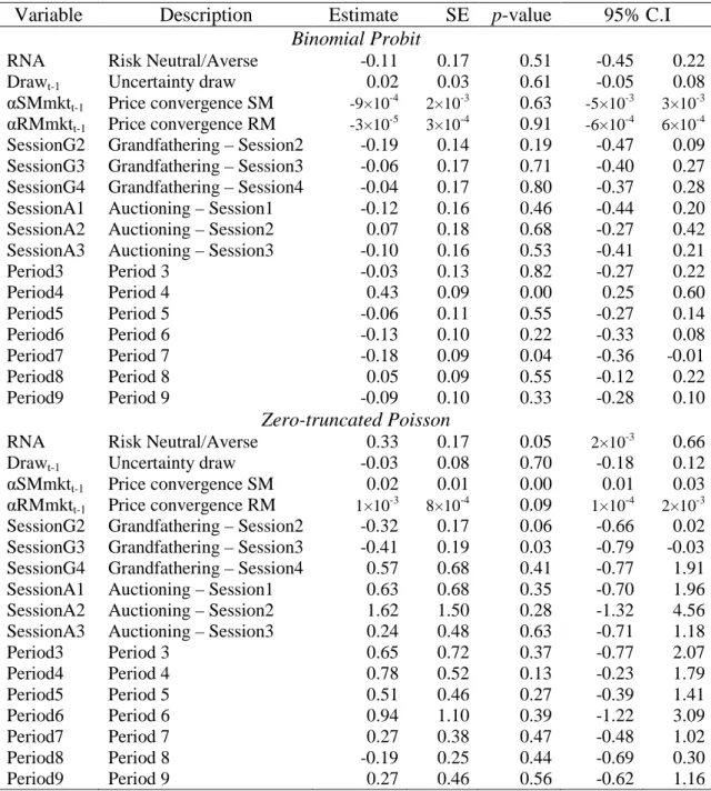
The overall likelihood function for the hurdle model is the product of two likelihoods, where the first likelihood corresponds to the probability that a subject banks a positive number of permits, and the second likelihood corresponds to the probability model for the distribution of nonzero counts only (Mullahy (1986)). Specifying the appropriate probability distributions for each part of the model allows us to obtain consistent and efficient estimates of the parameter vectors by separately maximizing each likelihood (McDowell (2003)). The dependent variable in the first part of the model is dichotomous in nature (either an individual banks permits or not), and a probit specification is used to estimate the parameters of this part. The dependent variable in the second part of the model consists of nonzero counts, and a zero-truncated Poisson specification is used to estimate the parameters of the second part. Due to the panel nature of our data, we use a “clustering” specification that controls for intra-subject correlation.
Independent variables include subjects’ risk preferences, session effects, performance measures of previous period markets, and the emissions’ fluctuation in the previous period. Subjects’ risk preferences are measured using a dummy variable taking the unit value if the subject is classified as risk neutral or risk averse based on the number of safe MPL choices (RNA). The effect of the uncertainty matrix implemented in the experiment is measured using the draw the subject faced in the previous round of the uncertainty resolution stage (Drawt-1), and the performance of previous period markets is measured using the root mean squared deviation of transacted from equilibrium prices in the secondary market (αSMmktt-1) and in the reconciliation market (αRMmktt-1).11 Finally, dummy variables for the sequence of periods within the treatments are also included to capture any adjustment patterns over time while remaining agnostic about appropriate learning models.
Table 4 provides maximum likelihood estimates of the hurdle model for these data. The top panel in the Table reports the estimates of the marginal effects of each explanatory variable on the dependent variable of the binomial probability model, and the panel at the bottom reports the estimates of the marginal effects of each explanatory
11
These variables are further explained in the subsections below. We report the results using convergence measures to Market price benchmarks, but all the econometric results are robust with respect to the use of the alternative System price benchmarks.
25
variable on the dependent variable of the truncated Poisson model. The focus variable is the RNA binary dummy since it measures the marginal effect of subjects’ risk preferences on banking behavior. It clearly has a statistically significant effect on the number of banked permits conditional on making any, and no effect at all on the decision to bank some permits or none. The latter result supports the non-parametric findings: risk loving and risk neutral/averse subjects choose to bank zero permits at similar rates (marginally higher for risk neutral/averse subjects, but far from achieving statistical significance). The two groups of subjects, however, differ on the amount of banked permits, conditional on there being any, as evidenced by the significant and positive marginal effect of RNA in the truncated Poisson equation. This is evidence that subjects’ risk preferences influence their banking behavior, and that the direction of the change in behavior is consistent with risk aversion being more conducive to higher levels of banked permits when someone does bank some permits.
One could hypothesize that an unexpected unit deficit in the previous uncertainty resolution round would impact positively the propensity to bank permits in the current period, but the results show no effect of the uncertainty draw on either the propensity to bank some permits or on the conditional amounts banked. Similarly, there is no clear adjustment pattern over time in either case, and behavior in the auctioning sessions does not differ from that observed in the omitted grandfathering session. Although previous measures of performance in trading markets have no effect on the current propensity to bank some permits, they do show an impact on the conditional amount of banked permits. The results suggest that slower contract price convergence in the main permit market (our secondary market - αSMmktt-1) positively impacts the amount of banked permits conditional on some banking. Albeit at a much smaller rate (almost negligible), and just on the boundary of statistical significance, slower contract price convergence in the reconciliation market (αRMmktt-1) also has a positive impact on conditional banking behavior. To a degree, these results provide empirical support to the argument that market participants base their current banking decisions on previous market permit prices (eg. Newell et al. (2005)).
26
Table 4 – Maximum likelihood estimates of the hurdle model of banking decisions
Variable Description Estimate SE p-value 95% C.I
Binomial Probit
RNA Risk Neutral/Averse -0.11 0.17 0.51 -0.45 0.22
Drawt-1 Uncertainty draw 0.02 0.03 0.61 -0.05 0.08
αSMmktt-1 Price convergence SM -9×10⁻⁴ 2×10⁻³ 0.63 -5×10⁻³ 3×10⁻³
αRMmktt-1 Price convergence RM -3×10⁻⁵ 3×10⁻⁴ 0.91 -6×10⁻⁴ 6×10⁻⁴
SessionG2 Grandfathering – Session2 -0.19 0.14 0.19 -0.47 0.09 SessionG3 Grandfathering – Session3 -0.06 0.17 0.71 -0.40 0.27 SessionG4 Grandfathering – Session4 -0.04 0.17 0.80 -0.37 0.28 SessionA1 Auctioning – Session1 -0.12 0.16 0.46 -0.44 0.20 SessionA2 Auctioning – Session2 0.07 0.18 0.68 -0.27 0.42 SessionA3 Auctioning – Session3 -0.10 0.16 0.53 -0.41 0.21
Period3 Period 3 -0.03 0.13 0.82 -0.27 0.22 Period4 Period 4 0.43 0.09 0.00 0.25 0.60 Period5 Period 5 -0.06 0.11 0.55 -0.27 0.14 Period6 Period 6 -0.13 0.10 0.22 -0.33 0.08 Period7 Period 7 -0.18 0.09 0.04 -0.36 -0.01 Period8 Period 8 0.05 0.09 0.55 -0.12 0.22 Period9 Period 9 -0.09 0.10 0.33 -0.28 0.10 Zero-truncated Poisson
RNA Risk Neutral/Averse 0.33 0.17 0.05 2×10⁻³ 0.66
Drawt-1 Uncertainty draw -0.03 0.08 0.70 -0.18 0.12
αSMmktt-1 Price convergence SM 0.02 0.01 0.00 0.01 0.03
αRMmktt-1 Price convergence RM 1×10⁻³ 8×10⁻⁴ 0.09 1×10⁻⁴ 2×10⁻³
SessionG2 Grandfathering – Session2 -0.32 0.17 0.06 -0.66 0.02 SessionG3 Grandfathering – Session3 -0.41 0.19 0.03 -0.79 -0.03 SessionG4 Grandfathering – Session4 0.57 0.68 0.41 -0.77 1.91 SessionA1 Auctioning – Session1 0.63 0.68 0.35 -0.70 1.96 SessionA2 Auctioning – Session2 1.62 1.50 0.28 -1.32 4.56 SessionA3 Auctioning – Session3 0.24 0.48 0.63 -0.71 1.18
Period3 Period 3 0.65 0.72 0.37 -0.77 2.07 Period4 Period 4 0.78 0.52 0.13 -0.23 1.79 Period5 Period 5 0.51 0.46 0.27 -0.39 1.41 Period6 Period 6 0.94 1.10 0.39 -1.22 3.09 Period7 Period 7 0.27 0.38 0.47 -0.48 1.02 Period8 Period 8 -0.19 0.25 0.44 -0.69 0.30 Period9 Period 9 0.27 0.46 0.56 -0.62 1.16
Notes: Because the variables Drawt-1, αSMmktt-1,and αRMmktt-1 have no antecedent for period 1, we lose
all first period observations. Thus, adjustment over time is normalized on period 2. Log-pseudolikelihood value for the binomial Probit (truncated Poisson) is -209.55 (-106.08); Wald test for the null hypothesis that all coefficients are zero in the binomial Probit (truncated Poisson) has a χ2 value of 68.28 (58.28) with 17 df, implying a p-value less than 0.001.
27
B. Market Performance
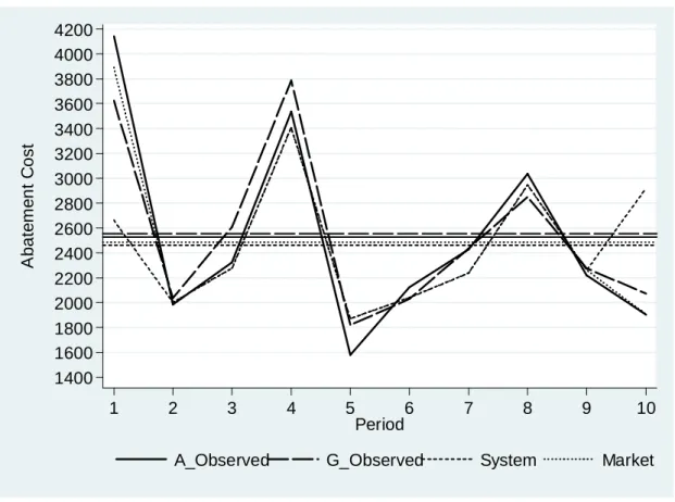
Figure 7 summarizes the main results (also shown in Table 5) from our sessions with respect to abatement costs. The horizontal lines show mean abatement costs pooled over the 10 trading periods for the auctioning treatment (A_Observed), and the grandfathering treatment (G_Observed). Also represented with horizontal lines are the mean minimum abatement costs pooled over the 10 periods for the computed benchmarks (System and Market). For both treatments, the overall observed means are closer to the Market benchmark than to the System benchmark. This result is to be expected given subjects’ banking behaviour. Although subjects’ banking behaviour did not conform to either of the System or Market specifications in none of the treatments, their behavior was on average closer to the latter.
It is clear from the Figure that, on average, observed behaviour in both treatments follows closely the theoretical optimum. As the Figure suggests, per period mean abatement costs in the grandfathering treatment are not statistically different from either the System or the Market optimums (based on the nonparametric Mann-Whitney test applied to per period means, for conventional significance levels). Thus, our second result is:
Result 2: Total abatement cost minimization is possible in the market under the EU ETS, having grandfathering as the initial allocation rule.
28 1400 1600 1800 2000 2200 2400 2600 2800 3000 3200 3400 3600 3800 4000 4200 A b a te m e n t C o s t 1 2 3 4 5 6 7 8 9 10 Period
A_Observed G_Observed System Market
Figure 7 – Abatement Costs
The same finding applies if we consider behaviour under the auctioning treatment compared to both benchmark values, and our third result is:
Result 3: Total abatement cost minimization is possible in the market under the EU ETS, having a 100% dynamic auction as the initial allocation rule.
Table 5 – Abatement cost benchmarks and observed values
Abatement Cost Benchmarks Observed Abatement Cost
BTU CCU Grandfathering Auctioning
Period System Market System Market
1 2663 3892 3236 4937 3623.25 4140.33 2 2002 2002 3057 3057 2038.00 1985.67 3 2277 2277 3308 3308 2608.00 2324.67 4 3408 3408 5019 5019 3785.75 3536.00 5 1871 1871 2895 2895 1817.75 1581.33 6 2040 2040 2876 2876 2029.75 2122.67 7 2237 2237 3082 3082 2435.25 2429.00 8 2947 2947 4156 4156 2852.00 3035.00 9 2261 2261 3116 3116 2274.75 2220.00 10 2918 1907 3804 3076 2073.25 1904.00
29
A commonly used performance/efficiency index (eg. Cronshaw and Brown-Kruse (1999), Godby et al. (1997)) rating the performance of observed behaviour against the optimal benchmarks is defined as:
) ( ) ( BTU CCU AbatCost CCU I − − =
where CCU stands for the command and control abatement costs (whereby subjects simply use their permits as allocated without engaging in banking nor trading permits) under uncertainty; BTU stands for the minimum abatement costs predicted with banking, trading, and uncertainty; and, AbatCost stands for the observed abatement costs.
This performance index is therefore a Cost Reduction index in that it measures the fraction of the maximum cost savings that could be achievable. Considering the data from the grandfathering treatment, the pooled (over the sessions and periods) cost reduction index is 90.8% and 93.5% for the BTU System and Market benchmarks, respectively. Considering the data from the auctioning treatment, the pooled cost reduction index is 93.4% and 95.7% for the BTU System and Market benchmarks, respectively. As implied from the discussion above, there are no statistically significant differences amongst these percentages, and they are all considerably high. These considerations allow us to state the following result:
Result 4: Total abatement cost within our EPM is equal in the grandfathering and auctioning treatments.
30
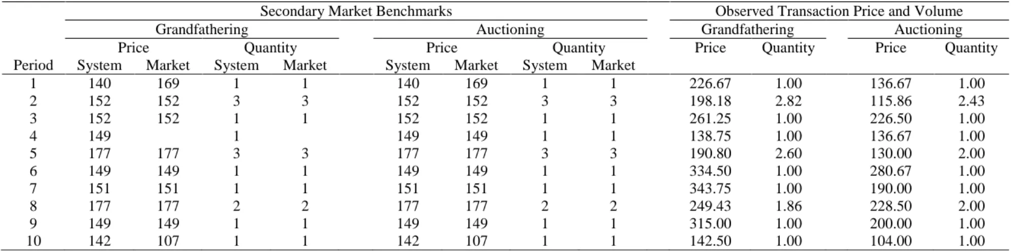
Table 6 – Secondary market benchmarks and observed transaction price and traded volume in the secondary market
Secondary Market Benchmarks Observed Transaction Price and Volume
Grandfathering Auctioning Grandfathering Auctioning
Price Quantity Price Quantity Price Quantity Price Quantity
Period System Market System Market System Market System Market
1 134 167 8 10 167 0 2 186.14 5.50 193.63 2.67 2 125 125 8 7 0 0 144.86 5.50 99.86 2.33 3 145 145 9 8 159 159 2 2 152.18 6.75 156.20 5.00 4 146 146 10 9 147 147 3 3 161.55 7.25 160.00 3.33 5 117 117 5 4 0 0 132.00 4.00 97.00 3.33 6 140 140 9 8 161 161 1 1 150.97 7.75 136.50 2.67 7 147 147 10 9 151 151 3 3 168.94 8.25 157.85 4.33 8 147 147 8 8 164 164 2 2 159.47 7.50 155.45 3.67 9 140 140 9 8 161 161 1 1 150.61 7.75 140.33 3.00 10 145 104 9 5 146 104 2 1 138.41 6.75 138.88 2.67
Note: Observed values in the cells are per period means over the sessions. Reported price benchmarks are midpoints of price tunnels encountered in some periods.
Table 7 – Reconciliation market benchmarks and observed transaction price and traded volume in the reconciliation market
Secondary Market Benchmarks Observed Transaction Price and Volume
Grandfathering Auctioning Grandfathering Auctioning
Price Quantity Price Quantity Price Quantity Price Quantity
Period System Market System Market System Market System Market
1 140 169 1 1 140 169 1 1 226.67 1.00 136.67 1.00 2 152 152 3 3 152 152 3 3 198.18 2.82 115.86 2.43 3 152 152 1 1 152 152 1 1 261.25 1.00 226.50 1.00 4 149 1 149 149 1 1 138.75 1.00 136.67 1.00 5 177 177 3 3 177 177 3 3 190.80 2.60 130.00 2.00 6 149 149 1 1 149 149 1 1 334.50 1.00 280.67 1.00 7 151 151 1 1 151 151 1 1 343.75 1.00 190.00 1.00 8 177 177 2 2 177 177 2 2 249.43 1.86 228.50 2.00 9 149 149 1 1 149 149 1 1 315.00 1.00 200.00 1.00 10 142 107 1 1 142 107 1 1 142.50 1.00 104.00 1.00
31
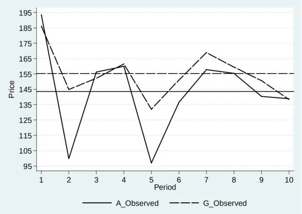
Figure 8 (and the summary statistics presented in Table 6) reveals that transaction prices in the secondary market for the grandfathering treatment are higher than those registered for the auctioning treatment. This result does not accord with prior expectations conditioned on an efficient performance of the initial auction format chosen to allocate permits. Despite these apparent differences, a two-sided Mann-Whitney test applied to per period means yields a p-value of 0.45, thereby failing to reject the null hypothesis that the two sets of independent values are from populations with the same distribution. Trading volumes, on the other hand, are statistically significantly different between the treatments (p-value=0.0003). In fact, Figure 9 shows that traded volumes in the secondary market of the auctioning treatment fall below those observed in the grandfathering treatment in each and every trading period, as predicted based on an efficient allocation of permits achieved by the considered dynamic auction for the initial permit allocation. This evidence is, therefore, mixed concerning the statement in our last hypothesis referring to behavior in the secondary market. The summary statistics reported in Table 7 reveal that transaction prices in the reconciliation market for the grandfathering treatment are higher than those registered for the auctioning treatment (a statistically significant difference; p-value=0.0342), and that traded volumes do not differ between the treatments (p-value=0.89). Given these observations, we state our fifth result as:
Result 5: Traded volumes (transaction prices) are lower, but transaction prices (traded volumes) are not different, in the secondary (reconciliation) market of the auctioning treatment compared with the grandfathering treatment.
32 95 105 115 125 135 145 155 165 175 185 195 P ri c e 1 2 3 4 5 6 7 8 9 10 Period A_Observed G_Observed
Figure 8 – Transaction Prices in the Secondary Market
0 1 2 3 4 5 6 7 8 9 Q u a n ti ty 1 2 3 4 5 6 7 8 9 10 Period A_Observed G_Observed
33
To complement the analysis of pricing behavior, we investigate whether the pattern of temporal play differs across the treatments. A common measure of pricing behavior (eg. Smith and Williams (1983)) is the root mean square difference between equilibrium and contract prices during each trading period, α. If there are nt transactions in period t, then αt is defined as:
∑
= − = nt i e i t t P P n 1 2 ) ( 1 αwhere Pe stands for the theoretical equilibrium price and Pi for the observed transaction prices in period t. Hence, α provides a measure of contract price convergence to the equilibrium prediction, and takes the 0 value when all contracts are made at the predicted equilibrium price (note that α is unbounded from above, with higher values indicating weaker convergence).
The analysis of the effect of time on the observed convergence measure is accomplished econometrically using the natural logarithm of α for each trading period in each session as the dependent variable in a linear regression model. Because we are modeling a dynamic adjustment process, we allow for heteroskedasticity across sections within the treatments, and also allow for the presence of first-order autocorrelation (specific to each session) in our estimation procedure. Explanatory variables include treatment effects, time effects, price convergence in the reconciliation market of the previous period, and their interactions. Treatment effects are measured using a binary variable taking the unit value for the auctioning treatment (Auctioning). Because behavior in the later part of the sessions (after some initial learning takes place) may better reflect any differences in the adjustment patterns between the treatments, time effects are measured using a binary variable taking the unit value for the last six trading periods within each session (Period>4). The variable αRMmktt-1 is the root mean squared deviation of transacted from equilibrium prices in the previous period of the reconciliation market, and purports to control for the influence of the reconciliation market outcomes on the subsequent main permit market.
34
Table 8 provides feasible generalized least squares (FGLS) estimates of the panel-data linear model for these data.12 The regression results show that both the differential intercept for the earlier periods and the differential intercept for the six later periods of the auctioning treatment are statistically significant at less than the bilateral 10% significance level, indicating better overall price convergence in the secondary market of the auctioning treatment compared with the grandfathering treatment. Following the adjustment procedure suggested by Halvorsen and Palmquist (1980), we compute price convergence to occur at a 60% ([exp(-0.92)-1]×100) faster rate in the first four periods of the auctioning treatment compared with the same first four periods in the grandfathering treatment. This difference in price convergence between the treatments is, ceteribus paribus, smaller in the final six periods, amounting to 34% ([exp(-0.92+0.59)-1]×100) faster in the auctioning treatment (bilateral p-value based on the Wald test for the appropriate composite linear hypothesis is 0.09).
The results also show that the pattern of price convergence differs between the final and the earlier trading periods in the grandfathering treatment. In this case, the differential intercept is given by the coefficient of the Period variable, indicating that, ceteribus paribus, price convergence occurs at a 34% ([exp(-0.41)-1]×100) faster rate in the six final periods of the grandfathering treatment, as one would expect if subjects adjusted their pricing behavior after some learning took place in the first rounds of the treatment. Interestingly, however, we do not observe the same effect occurring in the auctioning treatment. Given the adopted specification, such an effect is, all else the same, given by the sum of the coefficients on the Period and AuctPer variables, amounting to a statistically insignificant effect of a 20% slower convergence rate in the final rounds (bilateral p-value based on the Wald test for the appropriate composite linear hypothesis is 0.60, thereby failing to reject the null hypothesis of a null effect).
Turning to the effects of reconciliation market outcomes on the subsequent main permit market, the results indicate that weaker convergence in the former increases price convergence in the latter at a marginally significant (both in magnitude, and in
12
We report the results using convergence measures to Market price benchmarks, but the results are robust with respect to the use of the alternative System price benchmarks. The results are also robust to the use of the “panel corrected standard errors” (PCSEs) as an alternative to the FGLS estimation procedure (see Beck and Katz (1995) for a discussion).