IDENTIFICATION OF NAVEL ORANGE LESIONS BY NONLINEAR DEEP LEARNING ALGORITHM Guoliang Yang1 , Nan Xu2 , Zhiyang Hong

ISSN: 1809-4430 (on-line) www.engenhariaagricola.org.br

1 _{Jiangxi University of Science and Technology/ Ganzhou City, Jiangxi Province, China.} Received in: 4-18-2018

Doi: http://dx.doi.org/10.1590/1809-4430-Eng.Agric.v38n5p783-796/2018

IDENTIFICATION OF NAVEL ORANGE LESIONS BY NONLINEAR DEEP LEARNING

ALGORITHM

Guoliang Yang

1

_{, Nan Xu}

2*

_{, Zhiyang Hong}

1

2*_{Corresponding author. Jiangxi University of Science and Technology/ Ganzhou City, Jiangxi Province, China.}

E-mail: [email protected]

KEYWORDS

neural networks,

activation function,

plant image

classification, lesion

detection.

ABSTRACT

It is difficult for humans to recognize recessive diseases in navel oranges. Therefore, deep

neural networks are applied to plant disease identification. To improve the feature

extraction ability of convolutional neural networks, the Parameter Exponential Nonlinear

Activation Unit (PENLU) is proposed to replace the activated function of the neural

network. This function not only adds multiple parameters but also brings better

generalization ability to the neural network. In addition, the proposed function parameters

can be updated by the inverse Stochastic Gradient Descent (SGD) algorithm, which has

unparalleled advantages over the existing activated functions. The Residual Network

(ResNet), improved by PENLU, is applied to navel orange lesion recognition and

achieves the most advanced accuracy compared with traditional lesion recognition

methods. It is worth mentioning that the data set of navel orange leaf images proposed in

this paper will provide samples for subsequent research. The code and model are available

at the website https://github.com/xncaffe/caffe_penlu.

INTRODUCTION

It is well known that the navel orange originated in Brazil. Currently, they are planted in Brazil, Egypt (Abobatta, 2018), the United States and China (largest planting area) (Qiu et al., 2014). Its impact on the world agricultural economy is important. However, frequent citrus diseases have a great impact on the industry. For example, due to Huanglong disease in Xunwu County, China, from 2012 to 2015, the planted area of navel oranges was reduced from 400 km2 _{to 267 km}2 _{(Luo et al.,}

2017).In fact, in the early days, it was difficult to detect some hidden diseases with the naked eye. Professional testing equipment is difficult to popularize because of high prices and inconvenient use. These causes make it impossible to recover from losses after the discovery of disease. Therefore, a convenient and low-cost detection system to predict potential diseases in navel oranges is necessary that can be used to identify abnormalities when they cannot be distinguished by the naked eye. Currently,

artificial experience observation and field pathology detection are still the main means of prevention. However, the progress of computer vision provides new methods for plant disease recognition and extends the computer vision application market in agriculture. Many means for identifying and classifying plant disease, such as Threshold Processing (Barbedo, 2013), image classification (Pu, 2015), and semantic segmentation (Long et al., 2017), exist in the market. Digital image processing technology has shown great potential in the field of disease identification. The combination of digital image processing technology and other techniques can benefit feature extraction.

rather than hand-crafted features. Objects can be identified or detected through these features. LeNet (Lecun et al., 1998), which appeared in 1998, was considered to be the beginning of modern deep learning. By 2012, the deep convolutional neural network AlexNet (Krizhevsky et al., 2012) was proposed for the first time.The latest method of preventing overfitting "dropout" (Hinton et al., 2012) has been proposed and applied to neural network architecture to realize multi-GPU (Chen & Hang, 2008) parallel training. This is a significant innovation. The remarkable achievements in image processing have also spawned an increase in deep learning research. In addition, the continuous progress of modern computer hardware and large databases has provided great support for the development of deep learning.

In addition, as an important part of the deep neural network, the role of the activation function cannot be ignored. To solve the problem of the inadequate expression of the linear model, the activation function is added as a nonlinear factor in the neural network. By this function, the feature is preserved, the redundancy (useless or redundant features) in some data is removed and finally mapped out. From the early linear function and the threshold function to the subsequent Sigmoid Function, THINC (tanh), and ReLU (Rectified Linear Units) (Glorot et al., 2011), which are commonly used, the activation function of the neural network applies certain mathematical principles to achieve its effect. Two types of activation functions—_{the rectifier unit and the exponential}

unit have been directly invoked in the latest deep learning framework and have achieved the recognized effect. However, there is a gap between the exponential unit and the rectifier unit, resulting in nonuniformity between them. The rectifier unit can only express the linear function clusters well, and the exponential unit can only express the nonlinear exponential function cluster, which may destroy the representative capabilities of those architectures that use a particular activation function to some extent. According to the advantages and disadvantages previously discussed and based on the Parametric Rectified Linear Units (PReLU) (He et al., 2015) and the Exponential Linear Unit (ELU) (Clevert et al., 2015), the Parametric Exponential Nonlinear Unit (PENLU) is proposed as a new activation unit. This new function has more parameters than other activation functions and can cover the rectifier unit and the exponential unit so that it can convert between them. In addition, to achieving the goal of increasing the convergence speed with almost no effect on accuracy, it changes the linear state of the positive part of the function to nonlinearity. It is important that PENLU does not suppress the other part of the function with Batch Normalization (BN) (Ioffe & Szegedy, 2015).

One of the focuses of this paper is the new activation function—Parametric Exponential Nonlinear Function—which is used to improve the deep neural network, modify and alleviate the defects of the neural network activation layer, and improve the optimization

function of the activation function. Another focus is to classify and identify navel orange foliage by using a new method for improving deep neural networks to improve the defects of traditional plant disease identification methods. The structure of this paper is as follows: In the second chapter, a detailed introduction is given to works related to plant disease identification and activation function development. The method will be described in detail in the third chapter, including the improvement of the activation layer of the deep neural network and the principle of the deep convolution neural network for the recognition of navel orange leaves. In addition, it describes the specific experimental steps and the analysis of the experimental results in the fourth chapter. These experiments include the validation of the proposed activation function using the public database Cifar-10/100 and the use of improved deep convolution neural networks to identify navel orange diseases. Finally, the conclusions will be presented in the fifth chapter.

RELATED WORKS

As described in the previous chapter, the identification of navel orange lesions and the activation of the deep neural network used to identify the lesion are the focal points.

Identification of plant lesions in navel oranges

In the field of plant disease identification, scholars around the world have conducted considerable research. Pu (2015) used image segmentation to extract the tobacco leaf disease area, combined with the Double Coding Genetic Algorithm and Support Vector Machine (SVM), to identify the disease, which achieved a better result. Li et al. (2014) used red-edge near-infrared spectroscopy to establish a fruit leaf disease classification model. The classification accuracy was 90%. Similarly, Ma et al.

All samples were derived from web searches, and these categories were visually distinguishable and lacked credibility. Its architecture was very confusing and cannot be compared with the new architecture of PENLU in this paper.

Activation functions

The history of the activation function used by the artificial neural network is more than deep learning, but it has not been formally defined until recently (Gulcehre et al., 2016). The biggest influence of the activation function on the neural network is the ReLU (Glorot et al., 2011). The deep neural network has reached a higher level due to the extensive application of ReLU. ReLU is a piecewise linear function that keeps the negative input positive, and the output is zero. Because of this form, ReLU can reduce the problem of gradient disappearance and is suitable for deep neural network training. However, it has a potential drawback that once the gradient reaches zero, the neurons will never be activated. Maas et al. (2013) proposed the Leaky Rectified Linear Function (LReLU) for this defect, replacing the negative region of ReLU with a nonzero linear function. Subsequently, He et al. (2015) continued to extend LReLU (Maas et al., 2013) to PReLU, further changing the slope of the negative part to α and updating the value of α by the back-propagation of the neural network. This idea was a breakthrough that changed the nature of the previous activation function being unable to update parameters. The practice also shows that PReLU can lead to higher classification accuracy and rarely causes the risk of overfitting due to the introduction of parameters. In addition, Jin et al. (2015) proposed the S-shaped Leaky Rectified Linear Unit (SReLU) to study convex and nonconvex functions, which are inspired by the Weber-Fechner law (Weber, 1851) and Steven's law (Stevens, 1961). Subsequently, Clevert et al. (2015) proposed the Exponential Linear Unit (ELU), which uses an exponential function to modify the linear negative to nonlinear and then gives the negative part a soft saturation characteristic that results in more in-depth learning and better generalization performance. However, many studies (Clevert et al., 2015; Li et al., 2018) have shown that the use of ELU and BN (Ioffe & Szegedy, 2015) may impair classification accuracy. However, the very deep use of BN in the network is one of the main means for eliminating the risk of fitting, and the parameters of ELU cannot be updated in the reverse direction. In addition to the above deterministic activation function, there is a random version. Recently, Xu et al. (2015) proposed the Random-leakage Rectifier Linear Unit (RReLU). Although RReLU also has negative values and helps to avoid zero gradients, the difference is that the slopes of RReLU are not fixed or learned but random. Through this strategy, RReLU can reduce the overfitting risk to a certain extent.

MATERIAL AND METHODS

Deep learning methods are lacking in plant pathology identification. This chapter focuses on the principles of convolutional neural networks and the proposed activation functions. In addition, experimental planning and required materials are described.

Convolution neural network (CNN) implementation The advanced nature of CNNs refers to their ability to learn the advanced features of the image rather than the artificially extracted low-level features used in other image classification methods (Hinton et al., 2012). In a CNN, the convolution kernel in the hidden layer divides the image into feature maps. Through continuous segmentation and calculation of shared weights and offsets, we can learn useful information about the image. The feature maps are searched for the same characteristics of neurons, which are independently connected to different neurons in the lower layer. Basically, these feature maps are the result of applying convolution to the image, and the feature information is used to update the weights. Equation (1) and Equation (2) describe the construction formulas of the most important convolution and pooling layers in the CNN.

1 1

( 1) 0 0

( , ) tan (

i i

( , )

(

,

))

ij

R C

ij ij ijk i k

k K r c

o x y

h b

 

w r c o



x r y c

  











₍₁₎

where,

ij

o

_{- the}

j

_th feature map of the

i

th layer;

( , )

ij

o x y

_{- the element in}

o

ij;

tan ()

h

_{- the hyperbolic tangent function,}

ij

b

_{- the offset of the feature map}

o

ij.

In addition,

ij

K

_{- the feature set of the upper layer that}

connects

o

ij;

ijk

w

_{- represents the convolution kernel of}

o

ij

and

o

( 1)i j;

i

R - represents the row number of the convolution

kernel,

i

C _{- the number of the convolution kernel of this}

layer.

1 1

( 1) 0 0

( , ) tan (

N Ni i

(

,

))

ij ij ij i j i i

r c

o x y

h b g

 

o



xN r yN c

 











₍₂₎

Here,

1 2

l l



_{- the sampling area size;}

ij

The training process of the CNN can be divided into forward propagation and backward propagation. While the forward propagation is responsible for information transmission, the backward propagation is responsible for parameter updating. Equation (3), Equation (4) and Equation (5) indicate the basic principles of forward and backward propagation.

(1) (1) (2) (2) ( ) ( ) 1 2 1

( (

( (

)

) )

n n

)

i n n i

O F F





L

F F Xw b w b





L

w b



(3)

In which,

( )n

w

- the weight of the

n

th layer;

( )n

b

- represents the bias of the layer,

()

n

F

- the activation function of the

n

th layer.

2

1

₍

₎

2

i k ik ik

E





o



T

(4)

i

ik ik

ik

E

_o

_T

o









(5)

where,

i

E

- the error of the

i

th sample;

ik

o

- the actual output of the

k

th neuron of the

i

th

sample output,

ik

T

- the expected output of the

k

th neuron of the th

i

sample output.

Parametric exponential nonlinear unit

The PENLU is essentially the generalization of the ELU, which comes from the ELU and has all the advantages of the ELU but is different from the ELU. For the negative part, to bridge the differences between ELU and PReLU, additional parameter β can be added on the basis of ELU to control the shape change of ELU. However, the parameters of ELU can only be adjusted manually without the ability to update automatically, but PENLU can solve the deficiency of this part. For the positive part, the parameter η is added so that the linear part of the function is transformed into an exponential form. Unlike the Sigmoid and tanh functions, in which the gradient may disappear, PENLU does not exhibit this phenomenon because it does not have a right saturation property, and its derivative does not approach 0. By using the backward transfer SGD (Kaleem et al., 2015) algorithm, the parameters such as β and α are optimized so that they can be switched between the exponential unit and the rectifier unit at random, and the linear and nonlinear adjustment between them is possible. This design of PENLU is more flexible than ReLU, PReLU and ELU, and the latter can be regarded as a special case of PENLU. Thus, by constantly updating α, β and η, the space of the

negative part, including both linear and nonlinear, can be covered in a single active function module. Similarly, the positive part of the function can also adjust the coverage, while the other activation functions do not have this attribute.

Equation (6), Equation (7) and Equation (8) are the formula expressions for ReLU, PReLU and ELU, respectively.

( ) max(0, )

f x



x

₍₆₎

0

( )

0

x

x

f x

x

x







 

_



(7)

0

( )

(

x

1)

0

x

x

f x

e

x







 

_

_



(8)

From [eq. (6)], we can see that ReLU remains hard saturated at x < 0, so the negative part of the function has sparse properties. When x > 0, the derivative of the function is always 1 to ensure that ReLU prevents the gradient from decaying when the image information is positive, thereby alleviating the problem of gradient disappearance. While PReLU introduces the slope of the negative part of the learning parameter α adjustment function, α is updated by the reverse momentum method (He et al., 2015), and the channel sharing strategy is used to solve the overfitting risk caused by the increase of the parameter. The ELU summarizes the advantages and disadvantages of the rectifier unit and proposes that the negative part is modified to an exponential function with the left soft saturation characteristic; its total output mean is close to zero, so the convergence rate is faster.

The above three activation methods have a large impact on the development of neural networks. However, as mentioned above, after careful analysis, it is found that there is a commonality between the exponential unit and the rectifier unit, while there is a lack of unity in the theoretical unity. Therefore, we proposed that the Parametric Exponential Nonlinear Unit is used to achieve their unity goal, and the function belongs to the exponential unit of the full coverage of the rectifier unit in the form. The shape of the negative part of the ELU is adjusted on the basis of the ELU by introducing β, and then the values of α and β are adjusted to achieve the purpose of being freely convertible at the PReLU, ReLU and ELU. Equation (9) shows the result.

0 ( )

( x 1) 0

x x

f x

e x



 

  _{ }

 (9)

with the continuous deepening of training. In the case of need, the coverage of the PENLU can be expanded by adjusting the nonlinearity of the positive part to linear by adjusting η. Finally, the basic formula of the Parametric Exponential Nonlinear Unit is obtained, as shown in [eq. (10)]. Significantly, η should theoreticallyincrease the convergence speed properly when the initial value is adjusted within the range of 0 to 1 but is closer to 1, which would not affect the training accuracy. If it exceeds 1, the gradient rises and thus may lead to training divergence. In contrast, if it is far from 1 and closing to 0, it will lead to a large part of the feature information being filtered and lost, causing the rapid decline of the training accuracy and ultimately leading to the phenomenon of overfitting in the case of a larger learning rate. Similarly, because the negative part of PENLU does not have the same sparse property as ReLU, changing the initial value of α and β

will result in a change in the range of the function, which may cause the data to diverge to a certain extent. Theoretically, the negative result of the above possible situation is not caused by the increasing parameters because the results can be solved by adjusting the parameters. The correctness of the above theory will be demonstrated in subsequent experiments.

0, 0

1

( )

0

(

x

1)

x

x

f x

x

e

 







 



 

_





(10)

It can be seen from [eq. (10)] that when η = 1, the positive part of PENLU degrades to linear and denoted by

x. When β = 1, the negative part of PENLU degrades to ELU. In addition, the negative part of the function is approximately PReLU when β is very small. If the negative part of the function must be equivalent to ReLU, then α must equal 0.

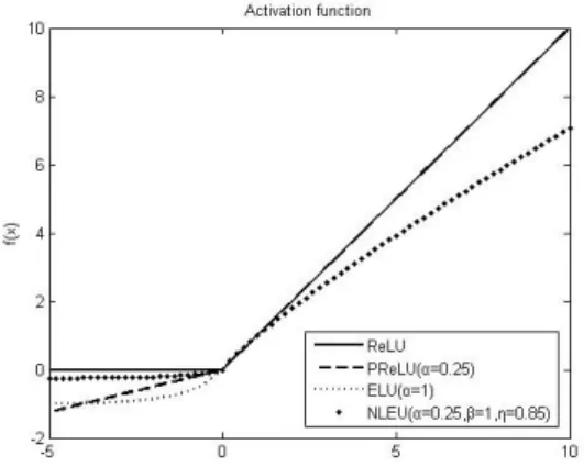
FIGURE 1. Graphics of activation functions.

Figure 1 shows the partial curves of the above four activation functions. For PENLU, the parameters α, β and

η are updated similarly to the convolution weight. As PENLU can be differentiated everywhere, the deep network using PENLU can engage end-to-end training. As shown in Eq. (11), the PENLU parameter updating rule is explained, in which the derivative is the gradient of the corresponding parameter.

( )

0

0

( )

1

0

0

0

( )

+

0

(ln )

0, 0

1

( )

0

0

(

) /

0, 0

1

( )

(

)

0

x

top

f x

x

f x

e

x

x

f x

x top

x

x top

x

f x

x

top x

x

f x

top

x

x





























 

_

_



_







 

_



_



 





 

_



_



 





 

_

_



_

g

（

）

₍₁₁₎

For parameter updating, the initial value of the parameter is not very important, but the effect of parameter initialization on the training results cannot be ignored. According to the theoretical basis of the former (He et al., 2015; Clevert et al., 2015), α generally uses the initial value of 0.25, 1 or 2 to set the experiment; β is set to 1 to initialize; η starts at 1 and gradually decreases by 0.05 each time. In the experiment, the effect of different initial values of each parameter on the result will be analyzed. In addition, this article emphasizes the importance of weight decay when the parameters of the active layer are updated. Unlike the rectifier unit, the effect of weight decay on the exponential unit cannot be ignored. In the case of nonlinearity, the exponential unit can alleviate the change range of the function by each reverse update by adding a weight attenuation theory and achieve the optimal fitting effect through gradual updating. However, this is not a necessary result because there are many factors that affect the results. We only emphasize that the weight decay of the parameters of the active layer has an effect on the outcome and that the effect may be negative or positive. The experiment will prove that PENLU is sensitive to weight decay.

In addition, inspired by the phenomenon that ELU cannot use BN, PENLU is theoretically able to use BN, which also greatly improves the optimization capabilities of the PENLU in a deeper network. The PENLU can be inherently divided into a structure as shown in Eq. (12) without regard to the positive partial nonlinearity. The data information flows out of the BN after flowing into the PReLU form, and the PReLU is effective for the BN, which can significantly improve the activation performance. This reflects the good fusion performance of PENLU. On the basis of Eq. (12), the nonlinear control of the positive part is introduced to represent the function completely.

(12)

we adopt a method that is similar to PReLU and a multi-parameter shared channel strategy for training. In each PENLU layer, the initialization increment of the parameter is up to twice the weight increment. For the number of weights of the many networks, the added parameters have little effect on the overall weight after sharing with the weight channel. If PENLU is used in training hundreds of thousands of big data, the likelihood of overfitting will be lower.

Datasets and implementation Datasets

Two public datasets and collected datasets on navel orange leaf images were used in this study. They are Cifar-10 and Cifar-100.The Cifar-10 database consists of 50,000 image training samples with 32×32 pixels and 10,000 image validating samples of the same size, which can be divided into 10 categories. These categories include airplanes, cars, birds, cats, deer, dogs, frogs, horses, boats and trucks. The number of pictures in Cifar-100 and the pixel size of each picture is the same as Cifar-10, but Cifar-100 contains a total of 100 categories.

Then, the collected navel orange leaf images were used to estimate the ability of the proposed method to identify navel orange lesions. The data were collected from middle-aged navel orange trees in Ganzhou, China. After an in-depth investigation of the navel orange garden, the navel orange leaves were photographed with a

13-megapixel mobile phone camera, and the model number of the mobile phone was the Xiaomi Redmi 3S. Then, these images were used as an experimental sample. To avoid the impact of the surrounding environment and improve the classification effect, the shooting process kept the shooting background uniform and made the focal length as even as possible. This ensured that the leaves occupied the central location of the picture and occupied more than 50% of the area of the entire image. The shooting process was all on the backside of the leaf, and the angle was vertical to verify the classification performance of the system in the case of insufficient illumination. Then, after removing the unqualified picture samples, leaves with yellowing disease, leaves lacking prime yellowing and normal fresh, 960 pieces were selected. Finally, all valid pictures of the training set and the validation set were scaled to a uniform pixel size of 256 × 256.

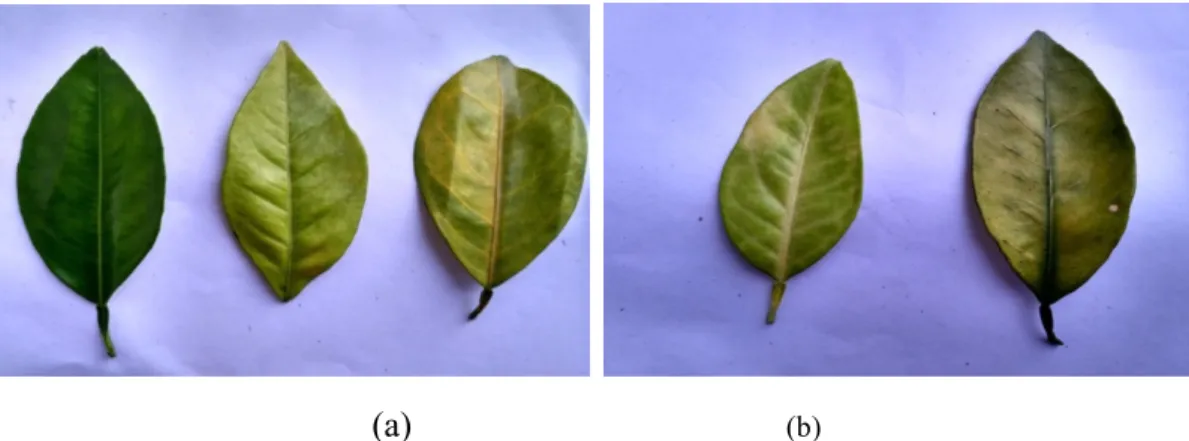
Images of navel orange leaves were collected in three categories (Figure 2(a)), and each category was divided into three parts: training (800 pieces), verification (150 pieces) and testing (10 pieces). In addition, 400 images of leaves of other plants (such as apples, pears, etc.) similar to navel orange leaves were collected. Similarly, these images were also divided into three parts: training (330 pieces), verification (60 pieces) and testing (10 pieces).

(a)

(b)

FIGURE 2. Leaves: (a) normal new leaves (left), lack of prime (middle), sick (right). (b): missing (left), sick (right).

Implementation

The experiment was divided into three parts. The first two sections verified the superiority of the proposed activation function on the Cifar-10/100. The last section shows the performance of the proposed method in the identification task of navel orange lesions.All experiments were conducted on the Caffe framework (Jia et al., 2014). In addition, all calculations were conducted on the

NVIDIA GeForce GTX 1080. The specific experiments

were conducted on the Cifar-10 and Cifar-100 datasets for different depths and types of architectures and different parameters of the same architecture. This paper

RESULTS AND DISCUSSION

Before the experiment of navel orange lesion identification, the actual effect of PENLU under different architectures and different databases should be verified first.

Verification of PENLU Experiments in Cifar-10

This experiment preliminarily verifies the effect of PENLU. Network in Network (NIN) (Lin et al., 2013) architecture and Dense convolutional Networks (DenseNet) (Huang et al., 2017) are used to classify training experiments in Cifar-10. The NIN architecture has nine convolution layers, including six convolutions with 1 × 1 kernel size and three Full Connection (FC) layers, which are easy to train and sufficient to comprehensively evaluate the effectiveness of the learning parameters. DenseNet is the latest CNN classification architecture, which can verify the effect of PENLU in advanced architecture.

The first step is the experiment on the NIN architecture. To ensure the effectiveness of the experiment, the rectifier unit ReLU, PReLU and exponential unit ELU are taken as the specific comparison object, and a comparative trial is carried out as the other parts of the network under the same conditions except for the activation layer. The weight of the architecture is initialized using the Gaussian (Yam et al., 2000) method, the corresponding standard deviation is 0.05, and the weighting of the parameters of the active layer does not use the decay strategy. Finally, 120,000 iterations were performed. The main variables of the experiment were the different initial values of the different parameters of PENLU. The learning rate’s attenuation methods needed to be adjusted according to the concrete conditions of the experiment, which can be set to step or multistep.The tests reproduced the NIN experiment in Cifar-10 without augmentation, and the accuracy of the result was 89.72% (ReLU results in Table 1), which is similar to the 89.59% of the original. Table 1 shows the specific experimental results.

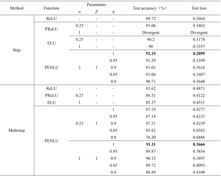
TABLE1. Experimental results on the Cifar-10 database

Method Function Parameters Test accuracy（%） Test loss

α β η

Step

ReLU - - - 89.72 0.3664

PReLU 0.25 - - 91.06 0.3462

1 - - Divergent Divergent

ELU 0.25 - - 90.2 0.3178

1 - - 90 0.3357

PENLU 2 1

1 92.15 0.2899

0.95 91.29 0.3399

0.9 91.01 0.3616

0.85 91.06 0.3487

0.8 90.71 0.3648

Multistep

ReLU - - - 83.62 0.4871

PReLU 0.25 - - 86.51 0.4122

ELU 1 - - 85.37 0.4511

PENLU

0.25 1

1 87.19 0.4277

0.95 87.14 0.4232

0.9 87.21 0.4239

0.85 85.82 0.8582

0.8 76.20 0.6886

1 1

1 91.11 0.3666

0.95 89.87 0.3854

0.9 90.15 0.3897

0.85 89.72 0.4093

It is worth mentioning that in the training of the PENLU architecture experiment, there were divergent situations that made it unable to train the results. This result appeared in the single step experiment; that is, we set the basic learning rate of 0.01 and decay once after 100,000 iterations. This phenomenon makes the PENLU architecture unable to continue training without iterating 100,000 times. The results of several experiments show that this phenomenon occurs at α = 0.25 or 1. Due to this situation, a set of comparative experiments was introduced, which was a multistep learning rate attenuation experiment. The focus of this additional experiment was to reduce the learning rate prior to the emergence of a phenomenon that could not be trained and then to decay once again after the 100,000 iterations. Through the analysis of the experimental observation, it was interesting that when η

decreases, the divergence phenomenon became more serious, which shortened the iteration number of divergence. If the initial value of α increased gradually, then the negative situation gradually decreased. When α

increased to 2, the situation was eliminated. The possible reasons for the emergence of this phenomenon are that reducing the area of the positive part will lead to the loss of positive information, thus accelerating the emergence of divergence. In contrast, if the area of the negative part increases, as much negative information as possible will be included to reduce the loss of information. These two aspects are considered from the overall output of the average close to zero, thus easing the emergence of divergence. However, when the negative region is larger, the result is better. When the α initial value is increased to 3, there is no significant difference from the result of α = 2. It shows that when the α initial value is increased to a certain condition, or when the negative part information is

contained as much as possible, the behavior of increasing the initial value of the parameters is invalid. The above analysis shows that the reason for the divergence is not due to the increased disadvantages of the parameters because such poor results can be solved by adjusting the parameters.

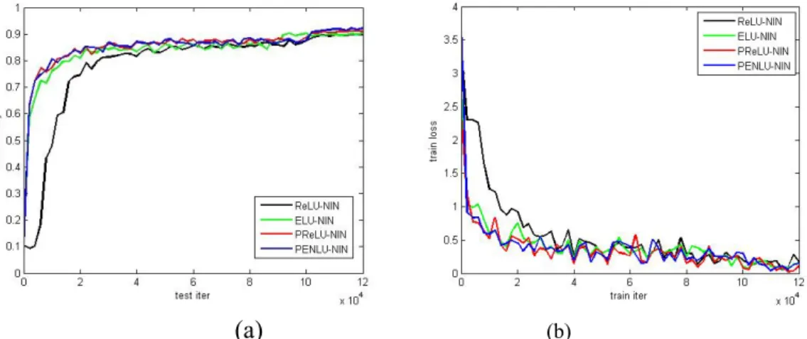
Analysis of the experimental results in Table 1 shows that PENLU presents an absolute advantage when the learning rate is decayed in advance, which proves that PENLU has the performance of high training accuracy in the case of a small learning rate. When α = 2 is used, PENLU has obvious advantages over ELU, ReLU and PReLU, and the final accuracy is significantly higher than the original architecture in Huang et al. (2017) and other activation architectures we built. All the analysis shows the benefits of increasing the parameters. In addition, a small decrease in η does not have a significant effect on accuracy and loss. In the case where the accuracy range is appropriate, the convergence rate can be increased by reducing η. The training log, which observes the different initial values of η, finds that when η = 1, the test accuracy increases to 0.9 after 102,000 iterations and η = 0.95 at 96,000iterations. When is further reduced to 0.85 at 76,000 iterations, at η = 0.8, 62,000 iterations are needed to improve the test accuracy to 0.9. This adjustment was not necessary for this experiment, but it cannot be ignored when training millions or even among hundreds of millions of data. It can also be found from Table 1 that the effect of changing the initial values of the ELU parameters on the results was almost negligible, whereas PENLU was the opposite. Figure 3 shows the test accuracy and training loss curves for the best results of ReLU, PReLU, ELU and PENLU.

(a)

(b)

FIGURE 3. The best results of NIN in Cifar-10 with different activation functions: test accuracy (a); training loss (b).

(a)

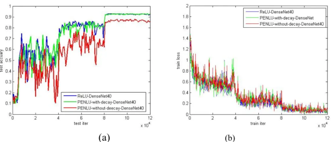
(b)

FIGURE 4. The change curve of the DenseNet architecture: test accuracy (a); training loss (b).

Then, the 40-layer DenseNet architecture was used for experimental verification. After using PENLU to improve the network, the accuracy of the test increased to 92.64%, which is higher than 92.26% of the reappearing experiment. This proves that PENLU can improve the network to a certain extent and achieve more advanced results. This also shows the excellent universality of PENLU, which still has the advantage of an advanced architecture. At the same time, it is worth noting that these experiments also indirectly prove that PENLU is effective for BN. Figure 4 shows the variation of training loss and test accuracy for DenseNet. This includes the original DenseNet and the structure after using PENLU to improve it.

As seen in Figure 4, when the parameters of the activation layer have weight decay, PENLU is slightly better than the original DenseNet. However, when the activation layer does not add the weight decay, the results obtained are much worse than the previous two, and this result is exactly the opposite of the phenomenon obtained in the later experiments (this can be seen in Table 2). The reason for this phenomenon may be related to the organization of the structure. Despite this result, PENLU remains competitive.

Experiments in Cifar-100

To observe the experimental results better, the NIN architecture was improved to achieve higher accuracy. First, a NIN unit was added to the original architecture,

and then the Full Connection layer that the original architecture does not have was increased to obtain a better classification accuracy. The first pooling layer of the architecture was changed to the average pool. In addition, the Dropout unit was added to solve the problem of increasing the loss caused by increasing the number of layers. Finally, we changed the weight initialization method to Xavier (Glorot & Bengio, 2010) to better match the activation function and optimize the convolution parameters through the experimental results. These improvements eventually brought the new architecture to 13 layers and were named MNIN. At the same time, we declared that all improvements were based on experimental results to verify PENLU from better results.

TABLE 2. Result of MNIN architecture on Cifar-100.

Function Parameters Weight decay

（Yes 1 or No 0）

MNIN

α β Test accuracy Test loss

ReLU - - - 67.04 1.3169

PReLU

0.25 - 0 68.27 1.4044

1 67.91 1.3846

1 - 0 Divergent Divergent

1 Divergent Divergent

ELU 0.25 - - 67.29 1.3684

1 - - 68 1.36

PENLU

0.25 1 0 67.99 1.386

1 67.29 1.3473

1 1 0 68.97 1.36

1 67.29 1.3392

2 1 0 69.48 1.3307

1 67.98 1.3052

* The parameter η in PENLU was fixed to 1 and was not learned, so it is not listed in the table.

(a)

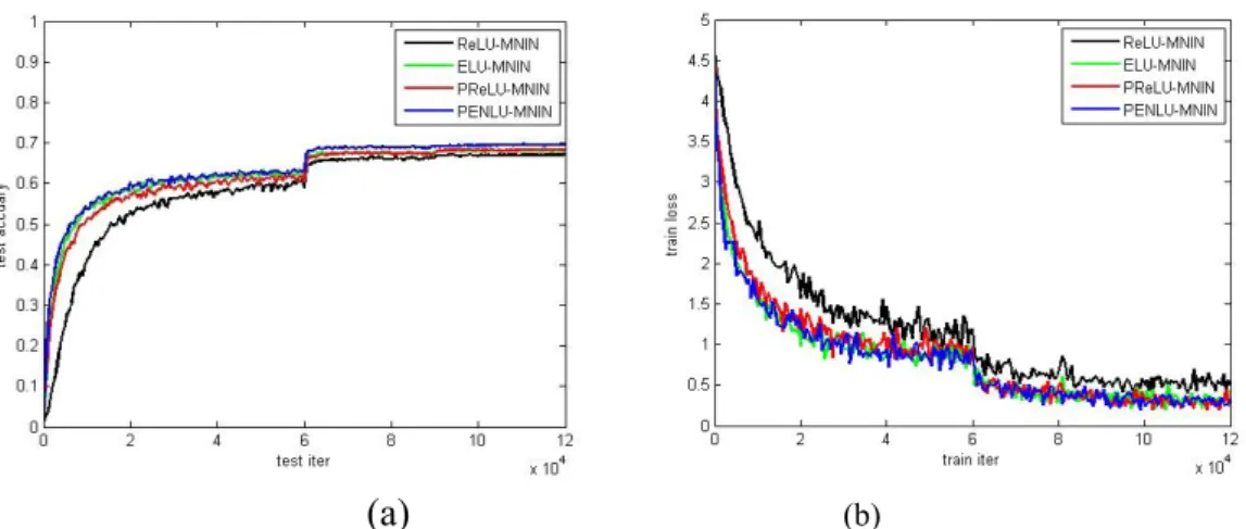
(b)

FIGURE 5. The change curve of MNIN architecture on Cifar-100 with different activation methods: test accuracy (a); training loss (b).

Table 2 shows that PENLU has the same superiority and that the decay of the parameter weight of the active layer will affect the final classification effect. Linking the results to Table 1 reveals that the effect of weight decay on the activation parameters can be positive for the accuracy of the classification. Although this effect performs very poorly in some cases, it can still be expressed. Figure 5

shows the optimal accuracy of the different activation methods in the MNIN architecture and the corresponding training loss curve. It can be seen in the figure that the training situation of PENLU is slightly better than ELU, which is obviously better than PReLU and ReLU.

FIGURE 6. A neural network architecture that identifies navel orange lesions.

To achieve better recognition, we used the 20-layer ResNet (He et al., 2016) non-bottleneck structure training model while adding the original architecture and the

corresponding PENLU architecture comparison

experiment. In the solver file, the batch size was set to 10, and the maximum number of iterations was set to 30,000. At the same time, the file specified that every traversal iteration operation was verified by a validation set once. In

the case of the output results, it was still specified in the file, including a training result after every 100 iterations, a test result after every 200 iterations, and an attenuation of the learning rate after every 10,000 iterations. The initial learning rate is 0.01, and the "multistep" approach was used in the strategy of learning rate decay. Table 3 shows the final training results.

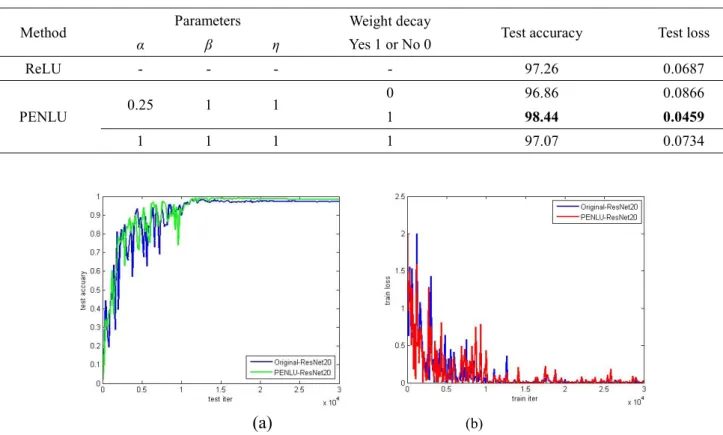
TABLE 3. The training result of using ResNet on the navel orange foliage image.

Method Parameters Weight decay

Yes 1 or No 0 Test accuracy Test loss

α β η

ReLU - - - - 97.26 0.0687

PENLU 0.25 1 1

0 96.86 0.0866

1 98.44 0.0459

1 1 1 1 97.07 0.0734

(a)

(b)

Table 3 shows that PENLU still has advantages. This advanced image recognition method has unparalleled superiority compared to traditional identification methods. Figure 7 shows the comparison results between the PENLU optimal and the original ResNet architecture for the test accuracy and training loss of navel orange foliage images.

To test the specific level of the practical application of the model, 40 test images were used to test the most

accurate model of the final improved ResNet training. The criteria for the evaluation were as follows. The picture was classified as the same category if the probability of testing was 80% or more. Therefore, it could perform a single or batch test after modifying and creating the relevant tools and code. After the model test, the final recognition rate reached 100%. No picture was discriminated incorrectly. To observe the update status of the model convergence, the weight diagrams are shown in Figure 8.

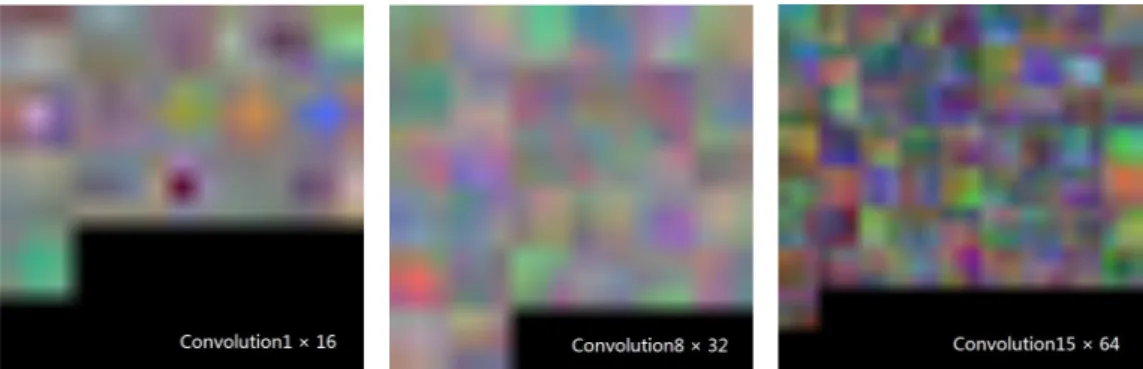
FIGURE 8. Visualization of weight in convolution layers.

The lower right corner of each graph in Figure 8 is marked by the weight view from which convolution layer is derived. It can be seen that the weight image aspect is very smooth and positively proves that the network convergence effect is very good.

FIGURE 9. Output feature maps of a leaf image after convolution layers.

Each of the small squares in Figure 9 shows the feature map of the corresponding filter. By observing each of these grayscale response feature maps, we can determine whether the structural design of the model (such as the number of channels per layer) is reasonable. If a large number of response feature maps are repeated or all close to 0, then the network efficiency can be increased by reducing the number of channels. From response feature maps, we can see that the model is very balanced, indicating that the number of filter channels is very reasonable.

CONCLUSIONS

Deep learning has great potential for agricultural computer identification and detection.

Our paper proposed improving the neural network architecture by the Parametric Exponential Nonlinear Unit. Using the deep learning framework as an experimental tool, we took local industrial navel orange lesion images as

As a continuation of this study, our team will continue to optimize the field of PENLU and plant disease identification. We strive to adjust the PENLU in the neural network to achieve the best results and focus the results of this study on practical applications.

ACKNOWLEDGMENTS

We would like to thank NVIDIA Corporation, Ningdu County government staff and the navel orange growers in Ganzhou of China for their support of this research. The study was supported by the National Natural Science Foundation of China (project number: 51365017) and the Jiangxi Polytechnic University Fund Project (project number: XS2017-S011).

REFERENCES

Abobatta W (2018) Improving Navel orange (Citrus sinensis L) productivity in Delta Region, Egypt. Journal of Microbiology Biotechnology & Food Sciences 1(1):36-38. DOI: https://doi.org/10.30881/aaeoa.00006

Alves WB, Rolim GDS, Aparecido LEDO (2017) Reference evapotranspiration forecasting by artificial neural networks. Engenharia Agrícola 37(6):1116-1125. DOI: https://doi.org/

10.1590/1809-4430-eng.agric.v37n6p1116-1125/2017 Barbedo JGA (2013) Digital image processing techniques for detecting, quantifying and classifying plant diseases. Springerplus2(1): 660. DOI:

http://doi.org/10.1186/2193-1801-2-660

Barbedo JGA (2016) A review on the main challenges in automatic plant disease identification based on visible range images. Biosystems Engineering 2016(144): 52-60. DOI: https://doi.org/10.1016/j.biosystemseng.2016.01.017 Chen WN, Hang HM (2008) H.264/AVC motion

estimation implmentation on Compute Unified Device Architecture (CUDA). In: International Conference on Multimedia and Expo. ICME. Hannover, IEEE, Proceedings…

Clevert DA, Unterthiner T, Hochreiter S (2015) Fast and accurate deep network learning by exponential linear units (elus). In: International Conference on Learning

Representations. San Juan, Neural Information Processing Systems Foundation, Proceedings…

Glorot X, Bordes A, Bengio Y (2011) Deep sparse rectifier neural networks.Jmlr W & Cp 15: 315-323. DOI:

https://doi.org/ 10.1.1.208.6449

Gulcehre C, Moczulski M, Denil M, Bengio Y (2016) Noisy activation functions. In: International Conference on Machine Learning. New York, IEEE, Proceedings… Glorot X, Bengio Y (2010) Understanding the difficulty of training deep feedforward neural networks. Journal of Machine Learning Research 9:249-256. DOI: https://doi.org/10.1.1.207.2059

Hinton GE, Srivastava N, Krizhevsky A, Sutskever I, Salakhutdinov RR (2012) Improving neural networks by preventing co-adaptation of feature detectors. In:

International Conference on Acoustics, Speech, and Signal Processing. Vancouver, IEEE, Proceedings…

He K, Zhang X, Ren S, Sun J (2015) Delving deep into rectifiers: surpassing human-level performance on imagenet classification. In: International Conference on Computer Vision and Pattern Recognition. Santiago, IEEE, Proceedings…

He K, Zhang X, Ren S, Sun J (2016) Deep Residual Learning for Image Recognition. In: International Conference on Computer Vision and Pattern Recognition. Las Vegas, IEEE, Proceedings…

Huang G, Liu Z, Weinberger KQ (2017) Densely Connected Convolutional Networks. In: International Conference on Computer Vision and Pattern Recognition. Hawaii, IEEE, Proceedings…

Ioffe S, Szegedy C (2015) Batch Normalization:

Accelerating Deep Network Training by Reducing Internal Covariate Shift.In: International Conference on Machine Learning. Lille, IEEE, Proceedings…

Jin X, Xu C, Feng J, Wei Y, Xiong J, Yan S (2015) Deep learning with s-shaped rectified linear activation units. In: Conference on Artificial Intelligence. Austin, AAAI, Proceedings…

Jia Y, Shelhamer E, Donahue J, Karayev S, Long J, Girshick R, Darrell T (2014) Caffe: Convolutional architecture for fast feature embedding. ACM 2014:675-678. DOI:

https://doi.org/10.1145/2647868.2654889

Krizhevsky A, Sutskever I, Hinton G E (2012) Imagenet classification with deep convolutional neural networks. Communications of the Acm 60(2):84-90. DOI: https://doi.org/10.1145/3065386

Kaleem R, Pai S, Pingali K (2015) Stochastic gradient descent on GPUs. ACM 2015:81-89. DOI:

https://doi.org/10.1145/2716282.2716289 Lecun Y, Bottou L, Bengio Y, Haffner P (1998)

Gradient-based learning applied to document recognition. Proceedings of the IEEE 86(11):2278-2324. DOI: http://doi.org/10.1109/5.726791

Li Y, Fan C, Wu Q, Ming Y (2018) Improving deep neural network with multiple parametric exponential linear units. Neurocomputing 301:11-24. DOI:

Lin M, Chen Q, Yan S (2013) Network in Network. In: arXiv. Available in: https://arxiv.org/pdf/1312.4400v3.pdf. Luo SL, Shen DC, Liu WJ, Xin KX (2017) Design of a Real Time Monitoring and Intelligent Diagnosis System of Huanglong Disease for Gannan Navel Orange.

Technological Development of Enterprise 36(7):16-17. DOI: https://doi.org/10.14165/j.cnki.hunansci.2017.07.005 Long J, Shelhamer E, Darrell T (2015) Fully convolutional networks for semantic segmentation. IEEE Conference on Computer Vision and Pattern Recognition 79:3431-3440. DOI: https://doi.org/10.1109/CVPR.2015.7298965 Ma H, Ji HY, Won SL (2014) Detection of Citrus Greening Based on Vis-NIR Spectroscopy and Spectral Feature Analysis. Spectroscopy and Spectral Analysis 34(10):2713-2718. DOI:

https://doi.org/10.3964/j.issn.1000-0593(2014)10-2713-06 Mei H, Deng X, Hong T, Luo X, Deng X (2014) Early detection and grading of citrus huanglongbing using hyperspectral imaging technique. Transactions of the Chinese Society of Agricultural Engineering 30(9): 140-147. DOI:

https://doi.org/10.3969/j.issn.1002-6819.2014.09.018 Maas L, Hannun Y, Ng Y (2013) Rectier Nonlinearities Improve Neural Network Acoustic Models. In:

International Conference on Machine Learning. Atlanta, IEEE, Proceedings…

Pu YX (2015) Image Searching Method of Tobacco Disease Based on Disease Spot Feature Fusion. Journal of Henan AgricuItural Sciences 44(2):71-76. DOI:

https//doi.org/10.15933/j.cnki.1004-3268.2015.02.015

Qiu JR, Fu YL, Liu QY, Li SY, Peng HJ, Pang ZH, Xu ZC (2014) Effects of Co-Substrates and Mixing Ratio on the Anaerobic Digestion of Navel Orange Waste. Advanced Materials Research 878:473-480. DOI:

https://doi.org/10.4028/www.scientific.net/AMR.878.473 Stevens SS (1961) To Honor Fechner and Repeal His Law. Science 133:80-86. DOI:

https://doi.org/10.1126/science.133.3446.80 Sladojevic S, Arsenovic M, Anderla A, Culibrk D, Stefanovic D (2016) Deep neural networks based recognition of plant diseases by leaf image classification. Computational Intelligence and

Neuroscience2016(6):1-11. DOI:

https://doi.org/10.1155/2016/3289801

Sindhuja S, Mari MJ, Sherrie B, Reza E (2013)

Huanglongbing (citrus greening) detection using visible, near infrared and thermal imaging techniques. Sensors 13(2):2117. DOI: https://doi.org/10.3390/s130202117 Weber EH (1851) Annotationes anatomicae et physiologicae: programmata collecta. Vol 6.

Xu B, Wang N, Chen T, Li M (2015) Empirical evaluation of rectified activations in convolutional network.In: arXiv. Available in: http://de.arxiv.org/pdf/1505.00853

Yang GL, Lu HR, Tang J, Wang YF (2016) Nonlocal image denoising with iterative log threshold weighted RPCA. Journal of Jiangxi University of Science and Technology 37(1):57-62. DOI:

https://doi.org/10.13265/j.cnki.jxlgdxxb.2016.01.011 Yam JYF, Chow TWS (2000) A weight initialization method for improving training speed in feedforward neural network. Neurocomputing 30(1):219-232. DOI: