The Analysis of Vibration Characteristics and Motion Stability of
the Tracked Ambulance Nonlinear Damping System
Meng Yang, Xinxi Xu, Chen Su
Institute of Medical Equipment, Academy of Military Medical Sciences,
Tianjin, China
Abstract
Considering the impact of the nonlinear stiffness, a 2 DOF dynamic nonlinear vibration model with cubic terms was established according to the structural feature and nonlinear behavior of the tracked ambulance. In the case of primary resonance and 1: 1 internal resonance, multiple scale method was used to obtain a first-order approximate solution for this model. Taking the parameters of the tracked ambulance for instance, the approximate solution was verified and the influence of the parameters on damping effect was investigated. Finally, the motion stability of the damping system was analyzed with singularity theory and the theoretical bases for improving efficiency of the damping system were provided. Keywords: Damping System; Cubic Nonlinearity, Multiple Scale Method; Internal Resonance; Stability
1. Introduction
The tracked ambulance can be delivered through a variety complex terrain and implement first aid to the sick and wounded. In order to achieve the safe transfer and implement first aid on the way, it is often necessary to demand the tracked ambulance has good mobility and meet the special needs of the sick and wounded of comfort. For the tracked ambulance is refitted by crawler chassis, he installation of the vehicle damping system becomes the main way to improve the ride comfort of the sick and wounded.
The tracked ambulance damping system is composed of the carriage, the stretcher base, the chassis and the nonlinear shock absorber. Hence, it can be easily converted into a multi-degree of freedom nonlinear vibration system. The use of the nonlinear vibration system presents various advantages, such as better
performance in the inhibition of broadband vibration, especially low-frequency vibration. However, complex mechanical properties usually exist in a nonlinear vibration system such as chaos and bifurcation, which makes it difficult to be analytic calculation and analysis, therefore approximate analytic algorithm widely used. Christopher Lee [4] investigated suspended,elastic cables driven by planar excitation with near commensurable natural frequencies in a 2:1 ratio. The first order analysis shows that there are saturation and jump phenomena and the first order analysis reveals that the cubic nonlinearities disrupt saturation. Li Jian et al [5] applied multiple scales method and Runge-Kutta to study the nonlinear vibration characteristics of the axial movement, multi-layered cylindrical shells made from composites. The results show some nonlinear properties of the system such as the phenomenon of internal resonance and indicate that excitation amplitude, damping and speed can affect the response amplitude, range of interval resonance and soft feature of the system. Zhang Xin et al [6] used average method to analyze piecewise nonlinear characteristics of the viscoelastic shocker absorber and the relationship of amplitude-frequency characteristics and system parameters. Li Xinye [7] used average method to study the possibility of delay feedback control over the gyroscope system under force. Tsuyoshi Inoue [8] investigates the vibration phenomena of the one-degree-of-freedom magnetically levitated system considering the effect of the nonlinearity of the electromagnet, using a shooting method.
scale method was used to obtain a first-order approximate solution of the differential equations. Taking the parameters of the tracked ambulance for instance, the accuracy of the approximate solution was established by compared to numerical results. The influence of the parameters on damping effect and motion stability was also investigated. Furthermore, the theoretical bases for improving efficiency of the damping system were put forward.
2. Damping System Physical Model
The tracked ambulance damping system is shown in Figure 1. Damping system is mainly composed of rubber damping shock absorber and zero stiffness damper. The linear model is used to describe the stiffness and damping of the rubber damping shock absorber. For zero stiffness damper, the damping is described by linear model and stiffness is described by positive and negative stiffness parallel model[9], shown in Figure 2.
Fig.1 Ambulance damping system
(1) Carriage(2)Stretcher base(3) Zero stiffness damper (4)Rubber
damping shock absorber(5) Coach chassis
Fig.2 Positive and negative stiffness parallel model
The stiffness, original length and initial deformation of horizontal spring, in Figure1, are defined as k, L and
. k0 Stands for the stiffness of vertical spring. Thevertical elastic restoring force of the model can be expressed in form
0
2
( ) [ ] (1)
1 ( / )
L x
f x k x k x
L x L
Using the Taylor series, I seek a second-order expansion in the form
2 4
2
1 1 13
1 ( ) ( ) (2)
2 24
1 ( / )
x x
L L
x L
Substitute the first two into the Eq.(1) result in
3
0 3
( ) ( ) (3)
2
k L k
f x k x x
L L
Hence, the restoring force of quasi-zero stiffness damper can be expressed in form
3
( ) s s (4)
f z K xK x
Where, s ( 0 )
k
K k
L
, 3
2 s
L k
K L
and is a small parameter.
According to the occupant of the vehicle ride(lying) comfort evaluation standards, occupant comfort is mainly affected by the vertical vibration acceleration. Ignoring the other two directions of vibration, the 2 DOF model of the tracked ambulance damping system is shown in Figure 3.
Fig.3 The 2 DOF damping system Including:
1
M —The quality of stretcher and decubital body;
2
M —The quality of carriage; s
K —The stiffness of quasi-zero stiffness damper;
1
C —The damping of zero stiffness damper;
2
K —The stiffness of rubber damping shock absorber;
2
C —The damping of rubber damping shock absorber; 1
The differential equations describing the motion of the damping system are
3
1 1 1(1 2) s( 1 2) s(1 2) 0 (5) M xC x x K x x K x x
3
2 2 1 1 2 1 2 1 2
2 2 3 2 2 3
( ) ( ) ( )
( ) ( ) 0 (6)
s s
M x C x x K x x K x x
C x x K x x
We rewrite the Eq.(5) and (6) as
2 3
1 1 1 1 2 1 1 1 2 1 1 2 2
2 2 2 2 1 3 2 2 1 3
2 1 2
2 2 ( ) (7)
cos 2 2
( ) (8)
x x l x u x u x b x x
x x f t u x u x l x
b x x
Where 2
1 Ks/M1
, l1Ks/M1 , 2u1C1/M1 ,
1 s/ 1
b K M , 2u2C1/M2 , 2
2 (K2 Ks) /M2
,
2 3 2 3
cos
f t K x C x ,2u3(C1C2) /M2,l2Ks/M2, 2 s/ 2
b K M .
3. Perturbation Analysis
Using multi-scale method, the dynamic response of damping system is solved. The new independent time scales
0,1, (9)
n n
T t n
are introduced where
represent a small positive parameter and Tn ,n0,1,are ‘slow’ time scaleswhich capture the response due to the nonlinearities, damping and external excitation. And we note that
0 1 2
2 2 2
0 0 1 1 0 2
2
(10)
2 ( 2 ) (11)
d
D D
dt
d
D D D D D D
dt
Where Dn / Tn,n0,1,. We expand the time-
dependent variable x1andx2 in powers of as
1 11( , )0 1 12( , )0 1 (12) x x T T x T T
2 21( , )0 1 22( , )0 1 (13) x x T T x T T
Then we substitute Eq.(10)-(13) into the Eq.(7) and (8), equate coefficients of like powers of
,and obtain the following:Order(0):
2 2
0 11 1 11
2 2
0 21 1 21 0
(14) 0
D x x
D x x
Order(1):
2 2
0 12 1 12 0 1 11 1 11 1 21
3 2 2 3
1 21 1 11 1 11 21 1 11 21 1 21
2 2
0 22 1 22 0 1 21 2 11 3 21
3 2 2 3
2 11 2 11 2 11 21 2 11 21 2 21 0
2 ( )
3 3
(15)
2 ( )
3 3
cos( )
D x x D D x u x u x l x b x b x x b x x b x D x x D D x u x u x
l x b x b x x b x x b x
f T
The solution of Eq. (14) can be expressed as
11 1 1 1 0 21 2 1 2 0 ( ) exp( )
(16) ( ) exp( )
x A T i T cc
x A T i T cc
To express 1:1 internal resonance and the nearness of the
excitation frequency to the first order natural frequency, we introduce two detuning parameter 1and 2defined by 2 1 1, 1 2.
Substitution of Eq.(16) and 2 11 , 1 2
into Eq.(15) leads to secular terms. Elimination of these secular terms leads to the two state equations
'
1 1 1 1 1 1 2 2 0
2 2
1 2 0 1 1 1 1 2 2 0 2
1 1 2 0 1 1 1 2 0 2
1 1 2 2 1 1 2 0 '
2 2 3 2 2 2 1 1 0
2 1 0 2
2 2 2 exp( )
exp( ) 3 3 exp( )
3 exp( ) 6 exp( )
6 3 exp(2 ) 0
2 2 2 exp( )
exp( ) 3
A i u A i u i A i T
l A i T b A A b A A i T
b A A i T b A A A i T
b A A A b A A i T
A i u A i u A i i T
l A i T b
2
1 1 0
2 2
2 2 2 2 1 2 0 2 1 1 2 2 1 2 2 0
2
2 1 2 0 2 1 1 1
(17) exp( )
3 3 exp( 2 )
6 6 exp( )
1
3 exp( ) exp( ) 0
2
A A i T
b A A b A A i T
b A A A b A A A i T
b A A i T f i T i T
Where An' D A1 n, 1.Introducing the polar form
1
exp( ) 2
n n n
A a i ,n1, 2
into Eq.(17) and separating the equation into real and imaginary parts results in the following four state equations,
' 3
1 1 1 1 1 1 2 2 1 2 1 2
2 2
1 1 2 1 1 2
1 3
cos sin sin
2 8
3 3
sin sin 2 0 (18)
8 8
a u a u a l a b a
b a a b a a
' 3 3
1 1 1 1 2 2 1 2 1 1 1 2
2 2 2
1 1 2 1 1 2 1 1 2
1 3 3
sin cos cos
2 8 8
9 3 3
cos cos 2 0 (19)
8 4 8
a u a l a b a b a
b a a b a a b a a
' 3
2 2 3 2 2 2 1 1 2 1 2 1
2 2
2 1 2 2 1 2
1 3
cos sin sin
2 8
3 3 1
sin 2 sin sin 0 (20)
8 8 2
a u a u a l a b a
b a a b a a f
' 3 2
2 2 2 2 1 1 2 1 2 1 2 1 2
2 2 3
2 1 2 2 1 2 2 2
1 3 3
sin cos cos
2 8 4
3 9 3 1
cos 2 cos cos
8 8 8 2
0 (21)
a u a l a b a b a a
b a a b a a b a f
where T021, 2 1T 1 1T2. At steady
state, ' ' 0 n n
a and the average Eq.(18)-(21) reduced to the form
2 2
1 1 1 1 2 2 1 1 2 1 1 2 3
1 2 1 2
3 3
cos sin 2 sin
8 8
3 1
sin sin 0 (22)
8 2
u a u a b a a b a a
b a l a
3 3 1 2 1 1 2 2 1 2 1 1 1 2
2 2 2
1 1 2 1 1 2 1 1 2
1 3 3
sin cos cos
2 8 8
9 3 3
cos cos 2 0 (23)
8 4 8
a u a l a b a b a
b a a b a a b a a
3 2
3 2 2 2 1 1 2 1 2 1 2 2
2 1 2 1 2
3 3
cos sin sin 2
8 8
1 3 1
sin sin sin 0 (24)
2 8 2
u a u a b a b a a
l a b a a f
3 2 2 2 1 2 1 1 2 1 2 1
3 2 2 2
2 2 2 1 2 2 1 2 2 1 2
1 3
( ) sin cos cos
2 8
3 3 3 9
cos 2 cos
8 8 4 8
1
cos 0 (25)
2
a u a l a b a
b a b a a b a a b a a
f
which provide the steady state amplitudes and phases.
4. Simulation Analysis
To establish the accuracy of the average equations and illustrate the relationship between the tracked ambulance parameters and damping effect, simulation analysis is performed for the parameters:M1180kg,M22000kg,
217582 / s
K N m , C14200N s m / , 0.1 ,
2 2200000 /
K N m,C219540N s m / , f 1500N .
For 1234.8rad s/ , the 1:1 resonance may occur.
In Figure 4, we show the comparison between numerical solutions, obtained by Runge-Kutta, and perturbation solutions.
Fig.4 Amplitude-frequency curve
In Figure 4, the trend and resonance position of perturbation and numerical solutions are the same. But the amplitudes are different. Because we only use the first-order approximation, which don’t affect our qualitative analysis of the behavior of the system dynamics. The damping system amplitude-frequency
diagram is similar to the linear system, where jump phenomenon does not occur.
Fig.5 The influence of excitation amplitude
Fig. 6 The influence of
1
Fig. 7 The influence of
2
C
Fig. 8 The influence of s
K
Fig. 9 The influence of 2
K
Figure 5-9 show the impact of the tracked ambulance parameters on the system vibration, where a1 and a2 represent the vibrating amplitudes of the carriage and the stretcher base. As can be seen from Figure 5, the amplitude of the excitation force has a great impact on
1
a and a2. Figure 6 and Figure 7 clearly demonstrate that he damping C1 has a great impact on the amplitude
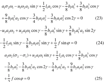
of a1, but little effect on the amplitude of a2 and damping C2 has a great impact on the amplitude of a1
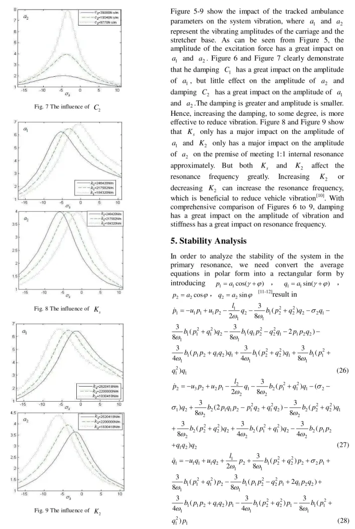
and a2.The damping is greater and amplitude is smaller. Hence, increasing the damping, to some degree, is more effective to reduce vibration. Figure 8 and Figure 9 show that Ks only has a major impact on the amplitude of
1
a and K2 only has a major impact on the amplitude of a2 on the premise of meeting 1:1 internal resonance approximately. But both Ks and K2 affect the
resonance frequency greatly. Increasing K2 or decreasing K2 can increase the resonance frequency,
which is beneficial to reduce vehicle vibration[10]. With comprehensive comparison of Figures 6 to 9, damping has a great impact on the amplitude of vibration and stiffness has a great impact on resonance frequency.
5. Stability Analysis
In order to analyze the stability of the system in the primary resonance, we need convert the average equations in polar form into a rectangular form by introducing p1a1cos( ) , q1a1sin( ) ,
2 2cos
p a ,q2a2sin [11-12]result in
2 2 1
1 1 1 1 2 2 1 2 2 2 2 1
1 1
2 2 2 2
1 1 1 2 1 1 2 2 1 1 2 2
1 1
2 2 2
1 1 2 1 2 1 1 2 2 1 1 1
1 1 1
2 1 1
2 2 2
2 3 2 2 1 1 2 1 1 1 2
2 2
1
3
( )
2 8
3 3
( ) ( 2 )
8 8
3 3 3
( ) ( ) (
4 4 8
) (26)
3
( ) (
2 8
)
l
p u p u p q b p q q q
b p q q b q p q q p p q
b p p q q q b p q q b p
q q
l
p u p u p q b p q q
q
2 2 2 2
2 2 1 1 2 1 2 1 2 2 2 2 1
2 2
2 2 2 2
2 2 2 2 2 1 1 2 2 1 2
2 2 2
1 2 2
2 2 1
1 1 1 1 2 2 1 2 2 2 2 1
1 1
2 2 2 2
1 1 1 2 1 1 2 2 1 1 2 2
1 1
3 3
(2 ) ( )
8 8
3 3 3
( ) ( ) (
8 4 4
) (27)
3
( )
2 8
3 3
( ) ( 2 )
8 8
3
b p q p p q q q b p q q
b p q q b p q q b p p
q q q
l
q u q u q p b p q p p
b p q p b p p q p q p q
2 2 2
1 1 2 1 2 1 1 2 2 1 1 1
1 1 1
2 1 1
3 3
( ) ( ) (
4 4 8
) (28)
b p p q q p b p q p b p
q p
2 2 2
2 3 2 2 1 1 2 1 1 1
2 2 2
2 3 2 2
2 1 1 1 1 1 2 2 2 2 1 2
2 2
2 2 2 2
1 2 2 2 2 2 2 1 1 2
2 2
2 1 2 1 2 2 2
3
( )
2 8 2
3 3
( 2 ) ( ) (
8 8
3 3
) ( ) ( )
8 4
3
( ) (29)
4
l f
q u q u q p b p q p
b p q q p q q b p q p
p b p q p b p q p
b p p q q p
Where the average equations become more complex and the exact analytical solution cannot be obtained. At steady state, p10,p2 0,q10 ,q20 and we use Newton Method to calculate the value of the equilibrium point of the average Eq.(26)-(29) by repeatedly changing the initial value of the equilibrium point. There are three sets of equilibrium points, as follows
1 { 3.9041, 1.2622, 2.0696,1.8797}
2 {12.1124, 7.7186, 13.7048, 10.4106}
3 { 10.9811, 6.7073,11.9741,8.9831}
The stability of the system at the equilibrium point is governed by the eigenvalue of the Jacobian matrix of Eq.(26)-(29) based on the singularity theory. The eigenvalues are obtained:
1 {-13.5988 +22.7426i, -13.5988 -22.7426i, -4.0362 + 5.5237i,-4.0362 - 5.5237i}
2 {-31.75 + 120.17i,30.18,-31.75 - 120.17i,-1.95}
3 {-28.95 + 103.88i,-1.70, -28.95 - 103.88i,24.33}
The Eq.(30) is the Jacobian matrix of the Eq.(26)-(29) at equilibrium point,where the expressions ofn iij( 14,
1 4)
j are given in appendix.
11 12 13 14 21 22 23 24 31 32 33 34 41 42 43 44
(30)
n n n n
n n n n
A
n n n n
n n n n
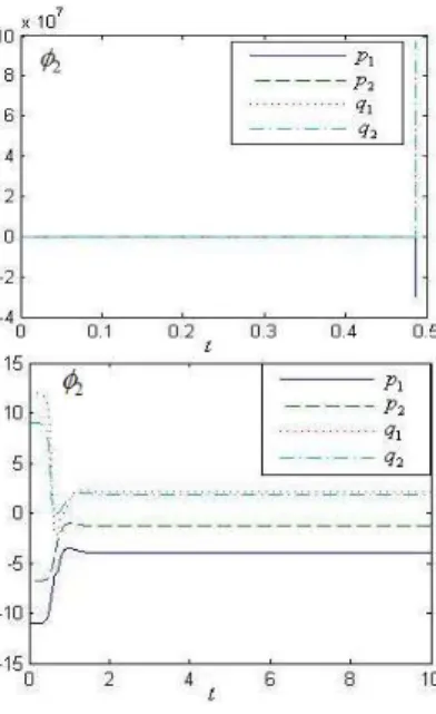
After singularity analysis, the system is only stable in the first equilibrium point. Since there is only one stable equilibrium point, the jump phenomenon does not occur. Use Runge-Kutta method to validate the singularity analysis. The Figure10 presents the final stable position of the Eq.(26)-(29) whose the initial values are the three equilibrium points.
Fig. 10 System stability location
Figure 10 clearly illustrates that the system is only stable in the first equilibrium point, which is in line with the actual system and diverges to infinity(Figure b) or converge to the stable equilibrium point(Figure c) at unstable equilibrium point. Therefore, the system is impossible to maintain a stable state in the unstable equilibrium point.
6. Conclusion
This paper established the dynamics model of a tracked ambulance damping system containing three nonlinear terms. We used Multiple Scales Method to investigate the dynamics model and obtain the average equations. The average equations were verified with the actual parameters. The influence of damping system parameters for the damping effect as well as the stability of the damping system were analyzed. The result explained the reasons that there is no jump phenomenon. This analysis method is suitable for multi-degree-of- freedom bearing motion system, particularly suitable for vehicle. The research results are valuable for the vehicle damping system design as well as forecast the damping system dynamic behavior.
Appendix:
1 2 1 1 2 2 1 1 2 1 1 1 11 1
1 1 1 1
3 3 3 3
4 4 4 4
b q p b q p b q p b q p
n u
1 2 2 1 1 2 1 2 1 1 1 1 1 2 12 1
1 1 1 1
3 3 (2 2 ) 3 3
4 8 4 2
b q p b q p p q b q p b q p n u
2 2
1 2 1 1 2 2 1 1 2 1 2
13 2
1 1 1
2 2 2 2 2 1 2 2 1 1 1 1 1
1 1 1
3 3 ( ) 3 ( )
2 8 4
3 ( ) 3 3 ( )
4 4 8
b q q b p q b p p q q n
b p q b q b p q
2 2 2 2 2 2
1 1 2 1 2 2 1 1 1 1 1 14
1 1 1 1 1
1 1 2 1 2 1 2 1
1 1
3 3 ( ) 3 ( ) 3
2 4 8 8 4
3 ( ) 3
4 2
l b q b p q b p q b q
n
b p p q q b q q
2 1 1 2 1 2 1 2 2 1 2 2 2 2 21 2
2 2 2 2
3 3 ( ) 3 3
4 4 2 4
b p q b q p p q b p q b p q
n u
2 1 1 2 2 1 2 2 2 2 1 2 22 3
2 2 2 2
3 3 3 3
4 4 4 4
b p q b p q b p q b p q
n u
2 2 2 2 2
2 2 1 2 1 1 2 2 2
23
2 2 2 2
2 2 1 2 2 1 2 1 2 2 2
2 2 2
3 3 ( ) 3 ( )
2 4 8 8
3 3 ( ) 3
2 4 4
l b q b p q b p q
n
b q q b p p q q b q
2 2 2
2 1 1 2 1 2 2 2
24 2 1
2 2 2
2 2 2 2
2 2 2 2 1 1 2 1 2 1 2
2 2 2
3 ( ) 3 3
8 2 4
3 ( ) 3 ( ) 3 ( )
8 4 4
b p q b q q b q
n
b p q b p q b p p q q
2 2
1 2 1 1 2 2 1 1 2 1 2
31 2
1 1 1
2 2 2 2 2
1 2 2 1 1 1 1 1
1 1 1
3 3 ( ) 3 ( )
2 8 4
3 ( ) 3 3 ( )
4 4 8
b p p b p q b p p q q n
b p q b p b p q
2 2 2 2 2 2
1 1 2 1 2 2 1 1 1 1 1 32
1 1 1 1 1
1 1 2 1 2 1 2 1
1 1
3 3 ( ) 3 ( ) 3
2 4 8 8 4
3 ( ) 3
8 2
l b p b p q b p q b p
n
b p p q q b p p
1 1 2 1 2 2 1 2 1 1 1 1 33 1
1 1 1 1
3 3 3 3
4 4 4 4
b q p b q p b q p b q p
n u
1 2 2 1 1 2 1 2 1 1 1 1 2 1 34 1
1 1 1 1
3 3 ( ) 3 3
4 4 4 2
b q p b q p p q b q p b q p
n u
2 2 2 2 2
2 2 1 2 1 1 2 2 2
41
2 2 2 2
2 2 1 2 1 2 2 1 2 2 2
2 2 2
3 3 ( ) 3 ( )
2 4 8 8
3 ( ) 3 3
4 2 4
l b p b p q b p q
n
b p p q q b p p b p
2 2 2
2 1 2 2 2 2 2 2
42 2 1
2 2 2
2 2
2 1 1 2 1 2 1 2
2 2
3 3 3 ( )
2 4 8
3 ( ) 3 ( )
4 4
b p p b p b p q
n
b p q b p p q q
2 2
2 1 1 2 1 1 1 2 2 1 2 43 2
2 2 2
2 2 2 2
3 3 ( 3 2 ) 3
4 8 2
3 4
b p q b p q p q b q p
n u
b p q
2 1 1 2 1 2 2 2 2 2 2 1 44 3
2 2 2 2
3 3 3 3
4 4 4 4
b p q b p q b p q b p q
n u
Acknowledgment
An acknowledgment should be shown to Dr. Weihua Su who helped us during the writing of this paper.
Reference
[1] Shafic S. Oueini, Char-ming Chin, Ali H. Nayfeh, "Dynamics of a Cubic Nonlinear Vibration
Absorber", Nonlinear Dynamics, 1999, Vol.20,No.3, pp.283-295.
[2] Shi Peiming, Liu Bin, Jiang Jinshui, "Stability and approximate solution of a relative-rotation nonlinear dynamical system with coupled terms",Acta Physical Sinica, 2009, Vol.58, No.4, pp.2147-2154. [3] Ali H. Nayfeh, Walter Lacarbonara, "On the
Discretization of Distributed-Parameter Systems with Quadratic and Cubic Nonlinearities", Non- linear Dynamics,1997,Vol.13,No.3, pp.203-220. [4] Christopher L.Lee, Noel C.Perkins, "Nonlinear
Oscillations of Suspended Cables Containing a Two-to-One Internal Resonance", Nonlinear Dynamics, 1992, Vol.3, No.6, pp.465-490.
[5] Li Jian, Guo Xinghui, Yang Kun, et al, "Study on The Nonlinear Vibration of Axially Moving Cylindrical Shells Made from Composites",Chinese Journal of Solid Mechanics, 2011, Vol.32, No.2, pp.176-185.
[6] Zhang Xin,Sun Dagang,Song Yang, et al, "Analysis of Damping Vibration Reduction Performance of Viscoelastic Shocker Absorber under Low Frequency and Heavy Loading", China Mechanical Engineering, 2012, Vol.23, No.14, pp.1651- 1656. [7] LI Xinye, Zhang Lijuan, Zhang Huabiao, "Forced
vibration of a gyroscope system and its delayed feedback control", Journal of Vibration and Shock, 2012, Vol.31, No.9, pp.63-68.
[8] Tsuyoshi Inoue, Yukio Ishida, "Nonlinear forced oscillation in a magnetically levitated system: the effect of the time delay of the electromagnetic force", Nonlinear Dynamics, 2008, Vol.52, No.1-2, pp.103-113.
[9] Peng Xian, Zhang Shixiang, "Nonlinear Resonance Response Analysis of a Kind of Passive Isolation System with Quasi-Zero Stiffness", Journal of Human University (Natural Sciences), 2011, Vol.38, No.8, pp.34-39.
[10] Su Chen, Xu Xinxi, Gao Zhenhai, et al, "Analysis on Two-Level Damping Efficiency and Recumbent Comfort for Tracked Emergency Ambulance", Journal of Vibration,Measurement &Diagnosis, 2012, Vol.32, No.5, pp.754-857,869.
[11] Liu Shuang, LI Yangshu, Liu Bin, et al, "Parametric Vibration Analysis and Control in Coupling Rotating Mechanical Drive System", China Mechanical Engineering, 2012, Vol.23, No.12, pp. 1461-1466.
[12] Liu Haoran, Zhu Zhanlong, Shi Peiming, et al, "Stability control of a coupled nonlinear torsional vibration system", Journal of Vibration and Shock, 2011, Vol.30, No.9, pp.140-144.
ergonomics.
Xinxi Xu received a master degree from Tianjin University, in 1989 and a Ph.D.degree from Tianjin University in2008. He is now the research associate and doctoral tutor of Institute of Medical Equipment, Academy of Military Medical Sciences, Tianjin, China. His research interests cover the structural dynamics,
vehicle NVH technology and ergonomics.