ESCOLA de PÓS-GRADUAÇÃO em ECONOMIA
Lucas Pimentel Vilela
Hypothesis Testing in Econometric
Models
Rio de Janeiro
2017
Hypothesis Testing in Econometric
Models
Tese
submetida
à
Escola
de
Pós-Graduação em Economia como requisito
parcial para a obtenção do grau de Doutor
em Economia
Área de concentração Econometria
Orientador: Marcelo J. Moreira
Rio de Janeiro
2017
I would like to express my sincere gratitude and appreciation to my advisor Marcelo J. Moreira, for his guidance and support during my Ph.D program. I also thank my coauthor of the …rst chapter, Benjamim Mills. I am in indebted to Donald Andrews and James Stock for their help, suggestions and contributions for the …rst chapter. I wish to thank Jose Diogo, Humberto Moreira, Caio Almeida, Kym Ardison, James Powell, Michael Jansson and Tiago Carvalho for valuable comments on the second and third chapter of this thesis.
This thesis is dedicated to my family: my father Geraldo Vilela Filho, my mother Ana Luiza Pimentel Vilela, my sisters Carolina Pimentel Vilela and Isabela Pimentel Vilela and my girlfriend Thais Buaiz Simao. Without their help and love, this work would not exist. I thank all my friends, who have always been by my side, in particular, my friends from EPGE and my hometown.
Esta tese contêm três capítulos. O primeiro capítulo considera testes de hipóteses para o coe…ciente de regressão da varíavel endógena em um modelo de variáveis instrumentais. O foco é em testes-t condicionais para hipóteses unilaterais. Trabalhos teóricos e numéricos mostram que os testes-t condicionais centrados nos estimadores de 2SLS e Fuller performam bem mesmo quando os instrumentos são fracamente correlacionados com a variável endógena. Quando a estatística F populacional é menor que dois, o poder é razoavelmente próximo do poder envoltório para testes que são invariantes a transformações que rotacionam os instrumentos (similares ou não similares). Este resultado é surpreendente considerando a baixa performance dos testes-t condicionais para hipóteses bilaterais apresentado em Andrews, Moreira, and Stock (2007). Estes testes possuem baixo poder porque as distribuições das estatísticas-t na hipótese nula são assimétricas quando os instrumentos são fracos. Explorando tal assimetria, nós propomos testes para hipóteses bilaterais baseados em estatísticas-t. Estes testes são aproximadamente não viesados e podem performar tão bem quanto o teste de razão de máxima verossimilhança condicional.
No segundo e no terceiro capítulos, nosso interesse é em testes do tipo maxmin e minimax regret para testes de hipóteses mais gerais. No segundo capítulo, nós apresentamos testes maxmin e minimax regret que satisfazem restrições mais gerais que as restrições de tamanho e de controle sobre todo o poder na hipótese alternativa. Restrições mais gerais nos possibilitam eliminar testes triviais e obter testes com propriedades desejáveis, como por exemplo não viés, não viés local e similaridade. Na sequência, nós provamos que ambos os testes existem e, sob condições su…cientes, eles são testes Bayesianos com priors que são solução de um problema de otimização, o problema dual. Na última parte do segundo capítulo, nós consideramos testes de hipóteses que são invariantes à algum grupo de transformações. Sob invariância, o Teorema de Hunt-Stein implica que a busca por testes maxmin e minimax regret pode ser restrita a testes invariantes. Nós provamos que o Teorema de Hunt-Stein continua válido sob as restrições gerais propostas.
No último capítulo, nós desenvolvemos um procedimento numérico para implementar os testes maxmin e minimax regret propostos no segundo capítulo. O espaço paramétrico é discretizado com o objetivo de obter testes de hipóteses com um número …nito de pontos. Nós provamos que, ao considerarmos partições mais …nas, os testes maxmin e minimax regret que satisfazem um número …nito de pontos possuem o mesmo poder na hipótese alternativa que os testes maxmin e minimax regret que satisfazem as restrições gerais. Portanto, nós podemos implementar numericamente os testes que satisfazem um número …nito de pontos como aproximação aos testes que satisfazem as restrições gerais.
Palavras-chave: Instrumentos fracos, variáveis instrumentais, testes invariantes, testes maxmin, testes minimax regret, testes não viesados, testes ótimos, testes similares.
This thesis contains three chapters. The …rst chapter considers tests of the parameter of an endogenous vari-able in an instrumental varivari-ables regression model. The focus is on one-sided conditional t-tests. Theoretical and numerical work shows that the conditional 2SLS and Fuller t-tests perform well even when instruments are weakly correlated with the endogenous variable. When the population F-statistic is as small as two, the power is reasonably close to the power envelopes for similar and non-similar tests which are invariant to rotation transformations of the instruments. This …nding is surprising considering the poor performance of two-sided conditional t-tests found inAndrews, Moreira, and Stock(2007). These tests have bad power because the conditional null distributions of t-statistics are asymmetric when instruments are weak. Tak-ing this asymmetry into account, we propose two-sided tests based on t-statistics. These novel tests are approximately unbiased and can perform as well as the conditional likelihood ratio (CLR) test.
The second and third chapters are interested in maxmin and minimax regret tests for broader hypothesis testing problems. In the second chapter, we present maxmin and minimax regret tests satisfying more general restrictions than the -level and the power control over all alternative hypothesis constraints. More general restrictions enable us to eliminate trivial known tests and obtain tests with desirable properties, such as unbiasedness, local unbiasedness and similarity. In sequence, we prove that both tests always exist and under su¢ cient assumptions, they are Bayes tests with priors that are solutions of an optimization problem, the dual problem. In the last part of the second chapter, we consider testing problems that are invariant to some group of transformations. Under the invariance of the hypothesis testing, the Hunt-Stein Theorem proves that the search for maxmin and minimax regret tests can be restricted to invariant tests. We prove that the Hunt-Stein Theorem still holds under the general constraints proposed.
In the last chapter we develop a numerical method to implement maxmin and minimax regret tests proposed in the second chapter. The parametric space is discretized in order to obtain testing problems with a …nite number of restrictions. We prove that, as the discretization turns …ner, the maxmin and the minimax regret tests satisfying the …nite number of restrictions have the same alternative power of the maxmin and minimax regret tests satisfying the general constraints. Hence, we can numerically implement tests for a …nite number of restrictions as an approximation for the tests satisfying the general constraints. The results in the second and third chapters extend and complement the maxmin and minimax regret literature interested in characterizing and implementing both tests.
Keywords: Instrumental variables regression, invariant tests, optimal tests, similar tests, unbiased tests, weak instruments, maxmin tests, minimax regret tests, most stringent tests.
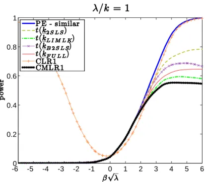
1.1 Asymptotic power of one-sided conditional tests ( = 0:5 and =k = 1). . . 24
1.2 Asymptotic power of one-sided conditional tests ( = 0:5 and =k = 2). . . 24
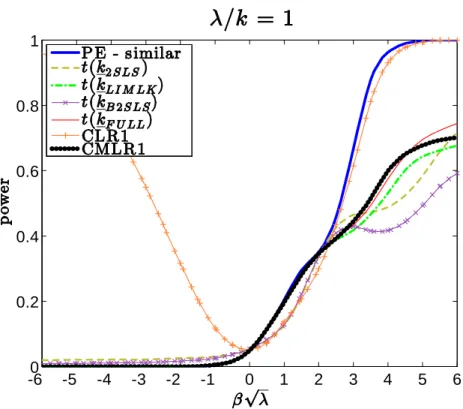
1.3 Asymptotic power of one-sided conditional tests ( = 0:9 and =k = 1). . . 25
1.4 Asymptotic power of one-sided conditional tests ( = 0:9 and =k = 4). . . 25
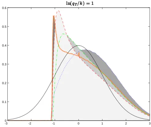
1.5 Probability density function for t(k) conditional on QT, where ln(qT=k) = 1:. . . 26
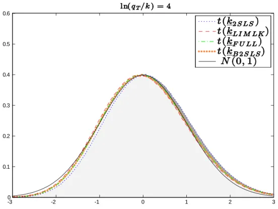
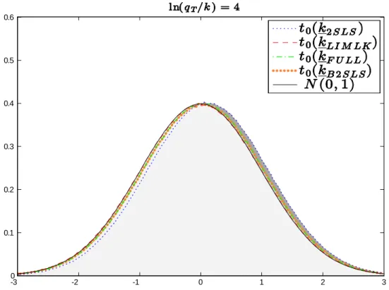
1.6 Probability density function for t(k) conditional on QT, where ln(qT=k) = 4:. . . 27
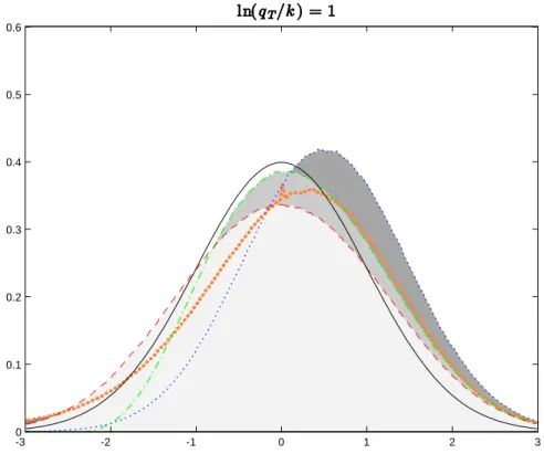
1.7 Probability density function for t0(k) conditional on QT; where ln(qT=k) = 1: . . . 28
1.8 Probability density function for t0(k) conditional on QT; where ln(qT=k) = 1: . . . 29
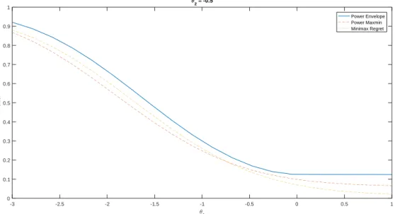
3.1 Power envelope and power of the Maxmin and Minimax Regret tests . . . 49
3.2 Power envelope and power of the Maxmin and Minimax Regret tests . . . 49
3.3 Power envelope and power of the Maxmin and Minimax Regret tests . . . 50
3.4 Power envelope and power of the Maxmin and Minimax Regret tests . . . 50
1 Tests Based on t-Statistics for IV Regression with Weak Instruments 10
1.1 Introduction. . . 10
1.2 Model and Su¢ cient Statistics . . . 11
1.3 Invariant Similar Tests . . . 12
1.4 The Conditional t-Tests . . . 14
1.5 Power Envelopes . . . 15
1.5.1 Similar Power Envelope . . . 15
1.5.2 Non-Similar Power Envelope . . . 17
1.6 Weak IV Asymptotics . . . 18
1.6.1 Tests for Unknown and Possibly Non-normal Errors . . . 19
1.6.2 Weak IV Asymptotic Results . . . 20
1.7 Strong IV Asymptotics. . . 21 1.7.1 Local Alternatives . . . 21 1.7.2 Fixed Alternatives . . . 22 1.8 Numerical Results . . . 23 1.9 Two-Sided Tests . . . 26 1.10 Uniform Convergence. . . 28 1.11 Empirical Example . . . 29
2 Maxmin and Minimax Regret tests satisfying general constraints 34 2.1 Introduction. . . 34
2.2 The Hypothesis Testing Problem . . . 35
2.3 The General Maxmin and Minimax Regret problems . . . 37
2.4 Characterization of the General Maxmin Test . . . 38
2.5 Characterization of the General Minimax Regret Test . . . 40
2.6 Invariant Hypothesis Testing . . . 41
3 Numerical Implementation of Maxmin and Minimax Regret Tests satisfying general con-straints 43 3.1 Introduction. . . 43
3.2 Discretization Method . . . 44
3.3 Power Convergence . . . 45
3.4 Maxmin and Minimax Regret Algorithms . . . 46
3.4.1 Maxmin Algorithm . . . 46
3.4.2 Minimax Regret Algorithm . . . 47
4 Appendix - Proofs 52 4.1 Proofs of Chapter 1 . . . 52
4.2 Proofs of Chapter 2 . . . 62
Tests Based on t-Statistics for IV
Regression with Weak Instruments
1.1
Introduction
Instrumental1variables (IVs) are commonly used to make inferences about the coe¢ cient of an endogenous
regressor in a structural equation. When instruments are strongly correlated with the regressor, the tests based on the score (also known as Lagrange Multiplier), likelihood ratio, and t-statistics are asymptotically equivalent. This trinity of tests provides reliable inference as long as the instruments are strong. When identi…cation is weak, however, the three approaches are no longer comparable. Kleibergen(2002) andMoreira
(2002) show that a Lagrange Multiplier (LM) statistic has a standard chi-square distribution regardless of the strength of the instruments.Moreira(2003) proposes a conditional likelihood ratio (CLR) test which is shown byAndrews, Moreira, and Stock(2006a) (hereinafter, AMS06a) to be nearly optimal. However, most results in the literature on the performance of tests based on the commonly used t-statistics are negative: Dufour
(1997) shows that standard tests based on t-statistics can have size arbitrarily close to one;Andrews, Moreira, and Stock(2006b) (hereinafter, AMS07) …nd that conditional t-tests are severly biased; and Andrews and Guggenberger(2010) prove that subsampling tests based on the Two-Stage Least Squares (2SLS) t-statistic do not have correct asymptotic size. SeeStock, Wright, and Yogo(2002),Dufour(2003), and Andrews and Stock(2007) for surveys on weak IVs.
In this chapter we present conditional one-sided t-tests for testing the null hypothesis H0 : = 0 (or
the augmented null H0 : 0) against the alternative H1 : > 0 (the adjustment for H1 : < 0
is straightforward). We consider t-statistics centered around the 2SLS, the limited information maximum likelihood (LIML), the bias-adjusted 2SLS (B2SLS), and the estimator proposed by Fuller(1977) (Fuller’s estimator). We also introduce conditional tests based on an one-sided score (LM1) statistic, a likelihood ratio (LR1) statistic for H0: = 0, and a likelihood ratio statistic (MLR1) for H0: 0. We develop a
theory of optimal tests for one-sided alternatives that parallels the two-sided results of AMS06a. We adopt the same invariance condition as in AMS06a and Chamberlain (2007) under which inference is unchanged if the IVs are transformed by an orthogonal matrix, e.g., by changing the order in which the IVs appear. We develop the Gaussian power envelope for point-optimal invariant similar (POIS) tests. When the null hypothesis is H0 : = 0, the conditional LR1 (CLR1) test is nearly optimal in the sense that its power
function is numerically close to the power envelope. For the more relevant null H0: 0, the CLR1 test
does not control size uniformly. The conditional t-tests have correct size and the one based on the 2SLS estimator numerically outperforms the conditional MLR1 (CMLR1) test. The LM1 test is a POIS test and does not have good power overall.
The good performance of the one-sided conditional 2SLS t-test is somewhat surprising considering the poor performance of two-sided conditional t-tests found in AMS07. We show that the poor performance is due to the asymmetric distribution of t-statistics under the null H0 : = 0 when instruments are weak. 1The present chapter is an extended version of the paperMills, Moreira, and Vilela(2014). Some results presented in this
chapter are derived in the early workAndrews, Moreira, and Stock(2004). We would like to express our sincere gratitude to Donald Andrews and James Stock for the contributions and suggestions.
We consider two methods to improve power for two-sided tests based on t-statistics. First, we propose novel tests which are by construction approximately unbiased. Second, we modify the t-statistics so that their null distribution is nearly symmetric. Both methods yield some t-tests whose power is close to the CLR test ofMoreira(2003). Hence, this chapter restores the triad of tests based on score, likelihood ratio, and t-statistics with reasonably good performance even when instruments are weak for two-sided hypothesis testing. By inverting the conditional t-tests, we can obtain informative con…dence regions around di¤erent estimators –including the commonly used 2SLS estimator.
The foregoing results are developed under the assumption of normal reduced-form errors with known covariance matrix. The …nite-sample theory is extended to non-normal errors with unknown variance at the cost of introducing asymptotic approximations. Under weak instrumental variable (WIV) asymptotics, the exact distributional results extend in large samples to feasible versions of the proposed tests. The …nite-sample Gaussian power envelopes are also the asymptotic Gaussian power envelopes with unknown covariance matrix. Under strong-IV asymptotics, we derive consistency even when errors are nonnormal and asymptotic e¢ ciency (AE) when errors are normal2.
The chapter is organized as follows: section1.2introduces the model with one endogenous regressor vari-able, multiple exogenous regressor variables, and multiple IVs. This section determines su¢ cient statistics for this model with normal errors and reduced-form covariance matrix. Section 1.3 introduces one-sided invariant similar tests. Section 1.4 focus on the one-sided conditional t-tests. Section 1.5 …nds the power envelope for similar and nonsimilar one-sided tests. Section1.6 adjusts the tests to allow for an estimated error covariance matrix and analyzes their asymptotic properties under weak IVs. Section1.7 obtains con-sistency and asymptotic e¢ ciency for one-sided tests. Section 1.8 compares numerically the power of the tests considered in earlier chapters under WIV asympotics. Section1.9introduces novel unbiased two-sided tests. Section1.10shows that the one-sided conditional t-tests based on 2SLS, LIML and Fuller estimators are asymptotic similar in a uniform sense. Section1.11presents con…dence intervals for returns to schooling using the data ofAngrist and Krueger (1991). An appendix at the end of the thesis contains proofs of the results. The supplement presents: power comparisons for di¤erent one-sided and two-sided tests; similar and non-similar power envelopes which are numerically very close (this fact further strengthens our optimality results).
1.2
Model and Su¢ cient Statistics
In this chapter we study a linear instrumental variable regression model with the objective of making inference about the coe¢ cient of the endogenous variable when the instruments are possibly weak. More speci…cally, we want to make hypothesis test of in the following linear model:
y1 = y2 + X 1+ u; (1.1)
y2 = Z + Xe 1+ v2; (1.2)
where y1; y2 2 Rn; X 2 Rn p; and eZ 2 Rn k are observed variables; u; v2 2 Rn are unobserved errors
(possibly correlated); and 2 R; 1; 12 Rp; and 2 Rk are unknown parameters. The matrices X and eZ
are taken to be …xed (i.e., non-stochastic) and Z := [X : eZ] has full column rank p + k.
In the …rst and main part of this chapter we are interested with one-sided hypothesis testing of the coe¢ cient :3
H0: = 0( or H0: 0) against H1: > 0 (1.3)
and in the last part we revise and deal with the two-sided hypothesis testing problem:
H0: = 0 against H1: 6= 0 (1.4)
It is convenient to transform the IV matrix eZ into a matrix Z which is orthogonal to X: Z0X = 0.
Since we are interested only in , we can decompose the IV matrix eZ = Z + PXZ := Me XZ + Pe XZ, wheree 2In principle, we could follow Cattaneo, Crump, and Jansson (2012) to obtain e¢ cient one-sided tests when errors are
nonnormal, but we do not pursue this line of research here.
MA:= I PA and PA:= A(A0A) 1A0 for any full column matrix A, and work with the model:
y1 = y2 + X 1+ u; (1.5)
y2 = Z + X + v2; (1.6)
where := 1+ (X0X) 1X0Z :e
Furthermore, the model can be rewritten as a reduced-form in the matrix form:
Y = Z a0+ X + V; (1.7)
where Y = [y1: y2] , V = [v1: v2] := [u + v2 : v2] , a := ( ; 1)0; := [ : ]; and := 1+ :
The reduced-form errors V are assumed to be independently and identically distributed (i.i.d) across rows. To obtain exact distribution of the tests, we assume that each row has a mean zero bivariate normal distribution with known 2 2 nonsingular covariance matrix := [!ij]i;j=1;2: As shown below, the normality
and the knowledge of assumptions can be relaxed when asymptotic approximations are considered. The probability model for (1.7) is a member of the curved exponential family, and low dimensional su¢ cient statistics are available. Lemma 1 of AMS06a shows that X0Y and Z0Y are independent and
su¢ cient for 0; 0 0 and ( ; 0)0, respectively. Since the assessment of the performance of the tests is by
its power we can focus only on tests based on the su¢ cient statistics, in particular on Z0Y . As shown by Moreira (2003), we can apply a one-to-one transformation to Z0Y that yields the k 2 su¢ cient statistic
[S : T ], where:4
S = (Z0Z) 1=2Z0Y b0 (b00 b0) 1=2and
T = (Z0Z) 1=2Z0Y 1a0 (a00 1a0) 1=2; (1.8)
where b0:= (1; 0)0 and a0:= ( 0; 1)0:
The distribution of the su¢ cient statistic [S : T ] is multivariate normal,
vec[S : T ] N (h ; I2k) ; (1.9)
with …rst moment depending on the following quantities:
h := (c ; d )02 R2 and := (Z0Z)1=2 2 Rk, (1.10)
where c := ( 0) (b0
0 b0) 1=2 and d := a0 1a0 (a00 1a0) 1=2:
1.3
Invariant Similar Tests
Seems natural to suppose that our decision to reject or not the null hypothesis is invariant to changes in the coordinate system of the instrumental variables, i.e the order in which each instrument appears, otherwise there is too much a priori information about the instruments and their relative relevance. The only exception to our knowledge that excludes speci…c instruments and consequently depends on the order in which the instruments appears is given byDonald and Newey(2001). In consequence we restrict our analysis to tests that are invariant to orthogonal transformations, i.e let be a [0; 1]-valued statistic depending on the su¢ cient statistics [S : T ] and F be a k k orthogonal matrix, so the tests considered are such (F S; F T ) = (S; T ).5
By Theorem 6.2.1 ofLehmann and Romano(2005) and Theorem 1 of AMS06a, a test is invariant if and only if it can be written as a function of
Q = [S : T ]0[S : T ] = S0S S0T T0S T0T =
QS QST
QST QT : (1.11)
The statistic Q has a Wishart distribution with rank one that depends on
(q) = h0qh = c2qS+ 2c d qST + d2qT; where (1.12)
q = qS qST qST qT 2 R
2 2:
4Henceforth, we use as the matrix square root as the (unique) symmetric square root.
5Moreira(2009) shows that the group of transformation on [S : T ] is isomorphic to a group of transformations on the original
Note that (q) 0 because q is positive semi-de…nite almost surely. The density of Q evaluated at (qS; qST; qT) is given by fQ(qS; qST; qT; ; ) = K1exp( (c2 + d2)=2) det(q)(k 3)=2 (1.13) exp( (qS+ qT)=2)( (q)) (k 2)=4I(k 2)=2( q (q));
where K1 is a constant, I ( ) denotes the modi…ed Bessel function of the …rst kind of order , and
= 0Z0Z 0: (1.14)
Examples of invariant test statistics are theAnderson and Rubin (1949), score and likelihood ratio stat-istics: AR = QS=k; LM = Q2ST=QT; LR = 1 2 QS QT + q (QS QT)2+ 4Q2ST : (1.15)
When the concentration parameter = (!22 k) is small, most test statistics are not approximately distributed
normal or chi-square. For example, under the weak instrument asymptotics ofStaiger and Stock(1997) where = C=pn, the LR statistic is not asymptotically pivotal. Its asymptotic distribution is nonstandard and depends on the nuisance and concentration parameter = (!22 k) under the null. Consequently, the null
rejection probability of the standard likelihood ratio test depends on the concentration parameter.
Moreira(2003) proposes similar tests which reject the null hypothesis when the test statistic exceeds a critical value that depends on QT:
(QS; QST; QT) > ; (QT); (1.16)
where ; (qT) is the 1 quantile of the distribution of conditional on QT = qT when = 0 :
P 0( (QS; QST; QT)) > ; (qT)) = : (1.17)
In practice, the critical value function ; (QT) of the conditional test given in (1.16) is unknown and must
be approximated. Given a statistic (QS; QST; QT) write it as a function of QS, S2 := QST=(jjSjj jjT jj)
and QT, by Lemma 3, (f) of AMS06a, (QS; S2) is independent of QT and has a nuisance-parameter free
distribution when = 0. The null distribution of (QS; S2) can be approximated by simulating nM C i.i.d
random vectors Si N (0; Ik) for i = 1; :::; nM C where nM C is large. The approximation to ; (QT) is the
1 sample quantile of f (S0
iSi; Si0e1 QT1=2; QT) : i = 1; :::; nM Cg and ej2 Rk euclidean vector with one in
the j-th coordinate and zero in the others.
We now introduce several new one-sided invariant similar tests for testing H0: = 0 (or H0: 0)
against H1: > 0. Each similar test will reject the null hypothesis when the one-sided statistic is larger
than the critical value function ; .
The k-class estimators (k) yield one-sided t-statistics:6
t (k) = (k) 0 u(k) [y02PZy2+ n (1 k) !22] 1=2 , where (1.18) (k) = y 0 2PZy1+ n (1 k) !12 y0 2PZy2+ n (1 k) !22 and 2u(k) = (1; (k)) (1; (k))0:
The nonstandard formula for the t-statistics in (1.18) arises here because we take as known (for present purposes only). The commonly used 2SLS estimator, the limited information maximum likelihood for known
6To avoid confusion with the number k of exogenous variables, we use k to de…ne Theil’s class of estimators rather than the
(LIMLK) estimator, the bias-adjusted (B2SLS) estimator proposed by Nagar (1959), and the estimator proposed byFuller(1977) belong to the k-class:
2SLS: k = 1;
LIMLK: k= kLIM LK = smallest root of j(Y0PZY =n + ) j = 0;
B2SLS: k = 1 + (k 2) =n; and Fuller: k = kLIM LK 1=n:
(1.19)
The …nite-sample properties of the estimators (k) depend on k. Consequently, the behavior of the t (k) statistics can be sensitive to the choice of k.
We construct two statistics from the likelihood of the model given in (1.7) with known. The …rst statistic is based on the standard LR statistic (i.e., 2 times the logarithm of the likelihood ratio) for testing H0: = 0: LR1 = 2 " sup 0 lc(Y ; ; ) lc(Y ; 0; ) # = R( 0) inf 0 R( ), where R( ) = b 0Y0P ZY b b0 b with b = (1; )0; (1.20)
and lc(Y ; ; ) is the log-likelihood function for known with all parameters concentrated out except . In
the Appendix, we show that R( ) and LR1 depend on the observations only through Q de…ned in (1.11) and
LR1 = LR 1( (kLIM LK) 0) + max f0; R( 0) R(1)g 1( (kLIM LK) < 0); (1.21)
where 1 ( ) is an indicator function and R(1) = lim !1R( ) (hence, R(1) equals R( ) with b replaced by
(0; 1)0). We show later that the CLR1 test’s power function P
; (LR1 > LR1; (QT)) is not monotonic for
< 0. Furthermore, the CLR1 test will not have correct size when the null hypothesis is H0: 0. The
second statistic is a standard LR statistic for testing H0: 0:
M LR1 = 2 " sup lc(Y ; ; ) sup 0 lc(Y ; ; ) # = inf 0 R( ) R( (kLIM LK)): (1.22)
In the Appendix, we show that
M LR1 = [LR max f0; R( 0) R(1)g] 1( (kLIM LK) 0) (1.23)
= LR1 max f0; R( 0) R(1)g : (For H1: < 0; the inequalities in (1.21) and (1.23) are reversed).
1.4
The Conditional t-Tests
We now elaborate more detailed expressions for the conditional t-tests. It is convenient to write
[S : T ] = (Z0Z) 1=2Z0Y 1=2J , (1.24)
where J is the orthogonal matrix
J = " 1=2b 0 p b0 0 b0 : 1=2a 0 p a0 0 1a0 # : (1.25)
From expressions (1.24) and (1.25), we obtain
Y0PZY = 1=2J QJ0 1=2; where 1=2J = c11 c12
We show that the t-statistics are then given by t (k) = (k) 0 u(k) [c221QS+ 2c21c22QST + c222QT + n (1 k) !22] 1=2 , where (1.27) (k) = c11c21QS+ (c12c21+ c11c22)QST+ c12c22QT + n (1 k) !12 c2 21QS+ 2c21c22QST + c222QT + n (1 k) !22 .
The term n (1 k) simpli…es for each estimator considered in (1.19). Algebraic manipulations show that 2SLS: n (1 k) = 0;
LIMLK: n (1 kLIM LK) = LR QS;
B2SLS: n (1 k) = 2 k; and
Fuller: n (1 k) = n (1 kLIM LK) + 1:
(1.28)
By writing QS = Q(k 1)+ LM = Q(k 1)+ LM 12 and QST = LM 1 Q1=2T , we can …nd the critical value
function for each t-statistic as in expression (1.17). For example, the conditional null distribution of the t-statistic based on the 2SLS estimator becomes
t (1) = (k) 0 u(k) h c2 21 Q(k 1)+ LM 12 + 2c21c22LM 1 qT1=2+ c222qT i 1=2, where (1) = c11c21 Q(k 1)+ LM 1 2 + (c 12c21+ c11c22)LM 1qT1=2+ c12c22qT c2 21 Q(k 1)+ LM 12 + 2c21c22LM 1 qT1=2+ c222qT , (1.29)
Q(k 1) has a chi-square distribution with k 1 degrees of freedom, and LM 1 has a standard normal
distri-bution.
1.5
Power Envelopes
In this section we address the question of optimal invariant similar and nonsimilar tests when the IV’s may be weak. To evaluate the performance of the novel one-sided conditional tests, we derive the power envelopes for similar and nonsimilar tests. The use of su¢ ciency and invariance reduces the dimension of the parameters from 1 + k + 2p for = ( ; 0; 0; 0)0 to just 2 for ( ; )0. The dimension reduction allows the power envelope
to meaningfully assess the performance of our one-sided tests. The envelope we derive here consists of upper bound for power and lower bound for either H0: = 0or H0: 0.
1.5.1
Similar Power Envelope
The following theorem is the main result of this section: Theorem 1 De…ne the statistic
LR (Q1; QT) = fQ1;QT(q1; qT; ; ) fQT(qT; ; )fQ1jQT(q1jqT; 0) ='1(q1; qT; ; ) '2(qT; ; ) ; (1.30) where '1(q1; qT; ; ) = exp( c2=2)( (q)) (k 2)=4I(k 2)=2 q (q) and '2(qT; ; ) = d2qT (k 2)=4 I(k 2)=2 q d2q T : (1.31)
Let ; (QT) be a shorthand for LR ; (QT). Then the following hold:
(a) For ( ; ) with > 0, the test that rejects H0 : = 0 when LR (Q1; QT) > ; (QT)
maximizes power over all level invariant similar tests.
(b) For ( ; ) with < 0, the test that rejects H0 : = 0 when LR (Q1; QT) < ;1 (QT)
Comments: 1. We denote the test that rejects the null when LR (Q1; QT) > ; (QT) as a
point-optimal invariant similar (POIS) test. We determine the power upper bound by considering the POIS tests for arbitrary values ( ; ) when > 0. The power upper bound is for similar tests for H0: = 0. We
do not impose the additional constraint that tests must have correct size, and so the upper bound could be conservative for H0: 0. We shall see later that even for small values of , some tests for H0 : 0
do reach the upper bound.
2. The test which rejects the null when LR (Q1; QT) < ;1 (QT) is called POIS0 test. We
determine the null lower bound by …nding the power of POIS0 tests for arbitrary values ( ; ) when < 0.
3. The power envelope is the union of the power upper bound and null lower bound. Both bounds are relevant because we would like to compare the probability of making the type I and type II errors for di¤erent tests.
4. The denominator '2(qT; ; ) does not depend on q1 and can be absorbed into the conditional
critical value. Thus, the test based on LR (Q1; QT) is equivalent to a test based on the numerator of
'1(q1; qT; ; ). For reasons of numerical stability, however, we recommend constructing critical values
using ln(LR (Q1; QT)).
We now show that such tests do not depend on , so that the POIS and POIS0 tests are of a relatively simple form. Using a series expansion of I(k 2)=2(x), we can write
'1(q1; qT; ; ) = 2 (k 2)=2exp( c2=2) 1 X j=0 ( (q1; qT)=4)j j! ((k 2)=2 + j + 1): (1.32)
The term '2(qT; ; ) can be written analogously.
The function '1(q1; qT; ; ) is increasing in (q1; qT) 0: As a result, for a …xed value of ; say > 0,
the optimal test for …xed alternative rejects H0: = 0 when
(Q1; QT) > ; (QT); (1.33)
where ; (QT) is a shorthand for ; (QT) as de…ned in (1.17). This POIS test is one-sided because it
directs power at a single point that is greater than the null value 0. An analogous argument shows that
the POIS0 test that minimizes rejection probabilities for …xed < 0 rejects H0when
(Q1; QT) < ;1 (QT). (1.34)
Corollary 2 For > 0, the POIS test based on (Q1; QT) is the uniformly most powerful test among
invariant similar tests against the alternative distributions indexed by f( ; ) : > 0g. For < 0, the
POIS0 test based on (Q1; QT) uniformly minimizes the null rejection probability among invariant similar
tests against the alternative distributions indexed by f( ; ) : > 0g.
Comments: 1. The form of the POIS test depends on the alternative . Hence, there does not exist a Uniformly Most Powerful Invariant (UMPI) test. Although the form of the POIS and POIS0 tests does not depend on , their power depends on the true value of . Hence, the power envelope depends on both parameters and .
2. A test based on (Q1; QT) is equivalent to a test that rejects when
P OIS1 = QS+ S2 p QS k p 2k + 2 > ; (QT); where = (2d =c )pQT,), (1.35)
and ; (QT) is a shorthand for P OIS1 ; (QT) de…ned in (1.17). This formulation of the test is convenient
because QS; S2; and QT are independent under = 0, which simpli…es the calculation of critical values.
3. Provided !12 !22 0 6= 0; the quantity d is a linear function of and equals zero if and only if
= AR; where
AR=
!11 !12 0
!12 !22 0
In this case, = 0 and P OIS1 reduces to QS=
p
2k; which is the AR statistic rescaled. Hence, the AR test, usually conceived as a two-sided test, is one-sided POIS against the alternative = AR:This …nding is in agreement with Chernozhukov, Hansen, and Jansson (2009) who use completeness of QT to show
that the weighted average power likelihood ratio (WAP-LR) tests of Andrews, Moreira, and Stock(2004) (hereinafter, AMS04) are admissible; see Moreira and Moreira(2013) on admissible WAP-LR similar tests without completeness.
4. The Locally Most Powerful Invariant (LMPI) test is the POIS test for local to 0 with > 0. This test is equivalent to the one-sided LM test that rejects H0 if
LM 1 = QST=Q1=2T > z ; (1.37)
where z is the 1 quantile of the standard normal distribution. Analogously, if is local to 0 with
< 0; then the LMPI test rejects H0if QST=Q1=2T > z .
5. The sign of in (1.35) can change as changes even for values on the same side of the null hypothesis because d is a linear function of : As a result, the form of the P OIS1 statistic (and the power envelope) changes dramatically as varies. The constant determines the weight put on the statistic S2. The optimal value of for small values of > 0has the wrong sign for large values of and vice versa.
This fact has adverse consequences for the overall one-sided power properties of POIS tests. 6. The optimal one-sided test for arbitrarily large rejects H0 if
QS+ 2(det( )) 1=2( 0!22 !12)QST > 1; (QT) (1.38)
for 1; ( ) as de…ned in (1.17). Remarkably, the same test is the optimal one-sided test for negative and arbitrarily large in absolute value for any . Consequently, the optimal two-sided test for j 0j arbitrarily large is the test in (1.38).
Corollary 2 shows that the POIS test for an alternative ( ; ) depends only on . Because the true parameter is unknown, we could construct an empirical version of the standardized optimal statistic:
eb= x0bQxb; (1.39)
where xb = (cb=jjhbjj; db=jjhbjj)0 and b is the maximum likelihood estimator of under H1: >
0. The
next theorem shows that the empirical POIS test is equivalent to those based on CLR1 test.
Theorem 3 The statistics eb and LR1 are equivalent up to strictly increasing transformations (possibly depending on QT). In particular,
P ; (eb> eb; (QT)) = P ; (LR1 > LR1; (QT)) : (1.40)
Comment: This theorem and Comment 5 of Corollary2indicate that the CLR1 test does not have correct size when the null hypothesis is H0 : 0 instead of H0 : = 0. See section1.8 below for numerical
simulations on size and power of the CLR1 test.
1.5.2
Non-Similar Power Envelope
Non-similar tests have null rejection probability below the signi…cance level for some values of the nuisance parameter . Due to the continuity of the power function, for such values of , the power of a non-similar test is less than the power of a similar test for alternatives close enough to the null hypothesis. However, for other values of , or for more distant alternatives, non-similar tests can have greater power than similar tests. For this reason, we also consider optimal invariant non-similar tests of the hypothesis H0 : = 0
against point alternatives.
Our construction of point-optimal invariant (POI) non-similar tests follows Section 3.8 ofLehmann and Romano(2005). Consider the composite null hypothesis
H0: ( ; ) 2 f( 0; ) : 0 < 1g; (1.41)
and the point alternative
Let be a probability measure over f : 0 < 1g and h be the weighted pdf, h (q) =
Z
fQ1;QT(q1; qT; 0; )d ( ) ; (1.43)
where fQ1;QT(q1; qT; ; ) is given in (1.13). The e¤ect of weighting by under the null is to turn the composite null into a point null, so that the most powerful test can be obtained using the Neyman-Pearson Lemma. Speci…cally, let be the most powerful test of h against fQ(q; ; ), so that rejects the null
when
N P (q) = fQ(q; ; )
h (q) > d ; ; (1.44)
where d ; is the critical value of the test, chosen so that N P (q) rejects the null with probability under
the distribution h .
If the test has size for the null hypothesis H0 in (1.41), i.e.,
sup
0 <1
P 0; (N P (Q) > d ; ) = ; (1.45)
then the test is most powerful for testing H0 against H1, and the distribution is least favorable; cf.
Thm. 3.8.1 and Cor. 3.8.1 ofLehmann and Romano(2005).
Given a distribution , condition (1.45) is easily checked numerically. What proves more computationally di¢ cult is …nding the distribution that satis…es (1.45). In the numerical work we consider distributions that put point mass on some point 0. In this case, we have
N P = fQ(q; ; ) fQ(q; 0; 0)
: (1.46)
Let R( 0; 0; ; j ; ) be the rejection probability of the test based on the statistic in (1.46) when the
true values are and . The numerical problem is to …nd the value of 0 such that the test has size .
Denote this value of 0 by LF0 ; then LF 0 solves R( 0; LF0 ; ; j 0; LF0 ) = and sup 0 <1R( 0 ; LF0 ; ; j 0; ) : (1.47)
If there is a LF0 ( 0; ; ) that satis…es (1.47), then the test based on N P LF
0 is the POI non-similar test.
The power upper bound for invariant non-similar tests is R( 0; LF
0 ( 0; ; ); ; j ; ) (an
ana-logous argument yields a null lower bound). We …nd numerically that the power envelopes for similar and non-similar tests are essentially the same, up to numerical accuracy. The reason for this is twofold. On one hand, the conditional critical values for the POIS tests depend on qT only weakly in the range of qT that is
most likely to occur under the alternative. Thus, the POIS tests are very nearly unconditional. On the other hand, the POI non-similar tests have null rejection rates that are very nearly equal to for all values of ; thus, the POI non-similar tests are very nearly similar. Because POI similar tests are nearly unconditional and the POI non-similar tests are nearly similar, the two types of tests have nearly the same rejection regions. An analogous result is described byAndrews, Moreira, and Stock(2008) for two-sided testing.
1.6
Weak IV Asymptotics
Here, we consider the same model and hypotheses as in section1.2, but with non-normal reduced-form errors with unknown covariance matrix. We show that the …nite-sample distribution of the tests and statistics holds asymptotically under the same high-level assumptions as in Staiger and Stock (1997). To model weak IV asymptotics and …xed alternatives (WIV-FA), we let be local to zero and the alternative be …xed, not local to the null value 0:
(b) is a …xed constant for all n 1:
(c) k is a …xed positive integer that does not depend on n:
We now specify the asymptotic behavior of the instruments, exogenous regressors, and reduced-form errors:
Assumption 1. n 1Z0Z !
pD for some positive de…nite (k + p) (k + p) matrix D.
Assumption 2. n 1V0V !
p for some positive de…nite 2 2 matrix :
Assumption 3. n 1=2vec(Z0V )!
dN (0; ) for some pd 2(k + p) 2(k + p) matrix ; where vec( ) denotes
the column by column vec operator.
Assumption 4. = D.
The quantities C; D; and are assumed to be unknown. AMS04 show that Assumptions 1-3 hold under general conditions. Assumption 4 holds under Assumptions 1-3 and homoskedasticity of the errors Vi, i.e.,
E(ViVi0jZi) = EViVi0= a:s.
We now introduce tests that are suitable for (possibly) non-normal, homoskedastic, uncorrelated errors with unknown covariance matrix. See AMS04 for tests and results for cases in which the errors are not homoskedastic or are correlated. For clarity of the asymptotics results, we write S; T; Q; etc. of section1.2, as Sn; Tn; Qn; etc.
1.6.1
Tests for Unknown
and Possibly Non-normal Errors
For feasible tests when we do not know the reduced-form error covariance matrix , we need to estimate consistently , and this is achieved by the estimator7
bn= n 1Vb0V ; where bb V = MZ;XY = Y PZY PXY; (1.48)
see Lemma 1 ofAndrews, Moreira, and Stock(2006b) (hereinafter, AMS06b).
Given that, we can replace by bn and obtain modi…ed versions of the statistics Sn; Tn; QS;n; QST ;n
and QT ;n: b Sn = (Z0Z) 1=2Z0Y b0 (b00bnb0) 1=2; b Tn = (Z0Z) 1=2Z0Y bn1a0 (a00bn1a0) 1=2, b QS;n = Sbn0Sbn, bQST ;n= bSn0Tbn and bQT ;n= bTn0Tbn: (1.49)
The feasible one-sided t-statistics for unknown are:
bt bk n = b(bk) 0 bu(bk)[y20PZy2+ n(1 bk) bw22] 1=2 , where b(bk) = y20PZy1+ n(1 bk) bw12 y0 2PZy2+ n(1 bk) bw22 , and b2u bk = 1; b(bk) bn 1; b(bk) 0 .
The values of bk are obtained from (1.28) after estimating :
2SLS: bk = 1
LIML: bk = bkLIM L= smallest root of j(Y0PZY =n bn) bnj = 0
B2SLS: bk = 1 + (k 2)=n Fuller: bk = bkLIM L 1=n:
(1.50)
The feasible bt bk
n statistics depend on bQ1;n; bQT ;n and bn in the same way the t(k) statistics depend
on Q1; QT and ; as described in previous sections. For all remaining test statistics, we just need to replace
QS; QST and QT by their analogues in which is estimated by bn. For example, the LR1 test statistic for 7This de…nition of b
nis suitable if Z or X contains a vector of ones, as is usually the case. If not, then bnis de…ned with
unknown is de…ned as in (1.21), but with QS; QST and QT replaced by bQS;n , bQST ;nand bQT ;n. We denote
the resulting test statistic by dLR1n. The analogue of M LR1 and LM 1 are denoted by \M LR1n and [LM 1n,
respectively.
The critical value function for each test statistic is simply ; ( bQT ;n), as de…ned in (1.17).
1.6.2
Weak IV Asymptotic Results
In this section we derive the limit distribution of each one-sided test present in the previous section. In particular, we show that all the tests converges in distribution to their respective …nite sample distribution under normality.
Under Assumptions WIV-FA and 1-4, Lemma 4 of AMS06a shows that
(Sn; Tn) !d(S1; T1); (1.51)
( bSn; bTn; bn) (Sn; Tn; ) !p0;
( bSn; bTn; bn) !d(S1; T1; );
where S1 and T1 are independent k-vectors which are de…ned as follows:
vec(NZ) N (vec(DZCa0); DZ); S1 = DZ1=2NZb0 (b00 b0) 1=2 N (c DZ1=2C; Ik), T1 = DZ1=2NZ 1a0 (a00 1a0) 1=2 N (d D1=2Z C; Ik); where DZ = D11 D12D221D21, D = D11 D12 D21 D22 ; D112 R k k; D 122 Rk p; and D222 Rp p: (1.52)
The matrix DZ is the probability limit of n 1Z0Z: Under H0: = 0; S1 has mean zero, but T1 does not.
Let
Q1 = [S1: T1]0[S1: T1];
QS;1 = S01S1; QST ;1= S10 T1; QT ;1= T10 T1;
S2;1 = S01T1=(jjS1jj jjT1jj); and
1 = C0DZC: (1.53)
By (1.52), we …nd that the …nite-sample distribution of (QS;1; QST ;1; QT ;1) is the same as that of (QS;n; QST ;n; QT ;n)
with n replaced by 1. Then the asymptotic distribution of the feasible tests and statistics are the same
as …nite-sample case:
Theorem 4 Under Assumptions WIV-FA, 1-4 and bk given in1.50: (a) (i) (bt(bk); t(k ); ( bQT ;n)) !d (t(k1); t(k ); (QT ;1)), (ii) ( [LM 1n; z ) !d(LM 1(Q1;1; QT ;1); z ), (iii) ( dLR1n; LR1; ( bQT ;n)) !d(LR1(Q1;1; QT ;1), LR1; (QT ;1)), (iv) ( \M LR1n; M LR1; ( bQT ;n)) !d(M LR1(Q1;1; QT ;1); M LR1; (QT ;1)). (b) (i) P (bt(bk) > t(k ); ( bQT ;n)) ! P (t(k1) > t(k ); (QT ;1)), (ii) P ( [LM 1n> z ) ! P (LM1(Q1;1; QT ;1) > z ), (iii) P ( dLR1n> LR1; ( bQT ;n)) ! P (LR1(Q1;1; QT ;1) > LR1; (QT ;1)), (iv) P ( \M LR1n > M LR1; ( bQT ;n)) ! P (MLR1(Q1;1; QT ;1) > M LR1; (QT ;1)).
(c)(i) P (t(k1) > t(k ) ; (QT ;1)) = P (LM 1(Q1;1; QT ;1) > z ) = for 2SLS, LIML and Fuller estimators
when = 0,
(ii) P (t(k1) > t(k ) ; (QT ;1)) for B2SLS estimator when = 0,
(iii)P (LR1(Q1;1; QT ;1) > LR1; (QT ;1)) = P (M LR1(Q1;1; QT ;1) > M LR1; (QT ;1)) = when = 0 and provided the signi…cance level 2 (0; 1=2)
Comments. 1. The t-statistics t(k1) are the limiting distribution of the t-statistics bt(bk).
2. Part (c) asserts that the conditional tests derived from the [LM 1n statistic and from the t-statistics
based in either the 2SLS, LIML or Fuller estimators are asymptotically similar at level .
3. The conditional B2SLS t-test is not asymptotically similar when instruments are weak because we set the term [y0
2PZy2 (k 2)!22]1=2 to zero if the term inside the square root is negative. However, this test
has correct size when = 0by the de…nition of the critical value function.
1.7
Strong IV Asymptotics
Two important large sample properties of tests are consistency: the power of the test under the alternative goes to one as the sample size increases; and asymptotic e¢ ciency (AE): the test uniformly maximize the asymptotic power among the asymptotically unbiased tests (seeLehmann and Romano(2005)). Given that, we analyze the asymptotic properties of the conditional tests based on [LM 1n, dLR1n, \M LR1n, and bt(bk)n
statistics for both local alternatives (SIV-LA) and …xed alternatives (SIV-FA). Under SIV-LA, we establish AE for the one-sided tests and under SIV-FA, we address consistency.
Before analyzing the asymptotic properties of the conditional one-sided tests, we need to establish the limit behaviour of the critical value functions under SIV-LA and SIV-FA. Under both asymptotics, SIV-LA and SIV-FA, QT diverges in probability to 1. We provide the following preliminary results when this occurs.
Lemma 5 Let z be the 1 quantile of the standard normal distribution. As qT !p1,
(a) for any k in (1.19), t(k ); (qT) ! z ,
(b) for 2 (0; 1=2), LR11=2; (qT) ! z . (c) for 2 (0; 1=2), M LR11=2; (qT) ! z .
Comment. As the sample size increases the statistic QT ;ndiverges to in…nity in probability which implies,
by the previous result, that the critical value functions of the tests considered converge in probability to the 1 quantile of the standard normal distribution.
1.7.1
Local Alternatives
For local alternatives, is local to the null value 0 as n ! 1.
Assumption SIV-LA.(a) = 0+ B=n1=2 for some constant B > 0:
(b) is a …xed non-zero k-vector for all n 1:
(c) k is a …xed positive integer that does not depend on n:
We use Lemma 6 of AMS06a to establish the strong IV-local alternative limiting distribution of tests. Under Assumptions SIV-LA and 1-4:
(Sn; Tn=n1=2) !d(SB1; T); (1.54)
( bSn; bTn=n1=2; bn) (Sn; Tn=n1=2; ) !p 0;
( bSn; bTn=n1=2; bn) !d(SB1; T; );
where SB1 and T are k-vectors de…ned as follows:
SB1 N ( S; Ik); where (1.55)
S = DZ1=2 B(b00 b0) 1=2 and
T = DZ1=2 (a00 1a0)1=2:
These de…nitions allow us to determine the behavior of the [LM 1n, dLR1n, \M LR1n, and bt(bk)n statistics
Theorem 6 Under Assumptions SIV-LA and 1-4: (a) if bk = k + Op(n 1) = 1 + Op(n 1); then bt(bk) = t (k) + op(1) !d( 0TSB1)=jj Tjj. (b) [LM 1n = LM 1n+ op(1) !d( 0TSB1)=jj Tjj, (c) dLR11=2n = LR1 1=2 n + op(1) !dmax f( 0TSB1)=jj Tjj; 0g, (d) \M LR11=2n = M LR11=2n + op(1) !dmax f( 0TSB1)=jj Tjj; 0g,
Comments. 1. The requirement k = 1 + Op n 1 is satis…ed by the k-class estimators considered.
2. The requirement bk = k + Op(n 1) allows us to show that the replacement of k by bk does not have any
asymptotic e¤ect for the t-statistics:
Together with Lemma5, Theorem6 yields the following optimality result for a sequence of experiments under SIV-LA and i.i.d normal errors with unknown covariance matrix . Under SIV-LA, the curvature of the model (1.7) vanishes asymptotically and standard local asymptotically normal (LAN) likelihood ratio theory is applicable. For one-sided alternatives, the usual one-sided LM test is AE under the SIV-LA asymptotics and i.i.d normal errors. The others one-sided tests that we propose are also AE.
Theorem 7 Suppose Assumptions SIV-LA and 1 hold and the reduced-form errors fVi : i 1g are i.i.d
normal, independent of fZi : i 1g with mean zero and p.d variance matrix which may be known or
unknown. Then the score test based on [LM 1n and the conditional tests based onbt(k)n are one-sided AE. If
2 (0; 1=2), the conditional tests based on dLR11=2n and \M LR11=2n are also AE.
1.7.2
Fixed Alternatives
We now analyze properties of the tests under strong IV …xed alternative (SIV-FA) asymptotics. This asymp-totic framework is novel in the weak-instrument literature and determines the consistency of tests.
Assumption SIV-FA.(a) 6= 0 is a …xed scalar for all n 1: (b) is a …xed non-zero k-vector for all n 1:
(c) k is a …xed positive integer that does not depend on n:
The strong IV-…xed alternative (SIV-FA) asymptotic behavior of tests depends on the random vector &k N (0; Ik) and
F A= 0DZ ; (1.56)
where DZ is de…ned in (1.52).
Lemma 8 Under Assumptions SIV-FA and 1-3, (i) (Sn=n1=2; Tn=n1=2) !p(c D1=2Z ; d D
1=2
Z ),
(ii) ( bSn=n1=2; bTn=n1=2) (Sn=n1=2; Tn=n1=2) !p0; and
(iii) if = AR and Assumption 4 holds, then Tn!d&k and bTn Tn!p0:
Lemma8allows us to determine the limiting behavior of the one-sided conditional tests based on bt bk
n,
d
LR1n, \M LR1n and [LM 1n statistics under SIV-FA asymptotics.
Theorem 9 Under Assumptions SIV-FA and 1-3,
(g) if bk = k + op(1) = 1 + op(1); bt(bk)=n1=2 = t (k) =n1=2 + op(1) !p c 1=2F A
(b00 b0=b0 b)1=2.
(b) if 6= AR, then [LM 1n=n1=2= LM 1n=n1=2+ op(1) !pc 1=2F A,
(c) if = AR and Assumption 4 holds, then [LM 1n=n1=2= LM 1n=n1=2+ op(1) !dc 0D1=2Z &k=jj&kjj;
(d) if > 0, dLR11=2n =n1=2= LR11=2 n =n1=2+ op(1) !pc 1=2F A, and (e) if < 0; dLR11=2n =n1=2= LR11=2 n =n1=2+ op(1) !p r max c2 ! 1 22; 0 1=2 F A, (f) if > 0, \M LR11=2n =n1=2= M LR11=2 n =n1=2+ op(1) !p r min c2; ! 1 22 1=2 F A,
(g) if < 0; \M LR11=2n =n1=2= M LR11=2
n =n1=2+ op(1) !p0,
Comments. 1. When 6= AR, the critical values of the conditional tests are either constants or converge in probability to constants as n ! 1 (see the comments following Lemma5). When = AR, the critical value functions of these tests (for each 0) are bounded. Therefore, this theorem addresses the consistency of each test.
2. The one-sided LM test rejects the null when [LM 1n=n1=2> z =n1=2. Because z =n1=2converges to zero
and the probability of c 0D1=2Z &k=jj&kjj being smaller than zero equals 50%, the LM1 test is not consistent
at = AR.
3. Part (d) shows that the CLR1 test is consistent against any alternative > 0 for the null hypothesis H0 : = 0. Part (d) shows that the CLR1 test asymptotically rejects the null with probability one for
some value of < 0. Hence, the CLR1 test has asymptotic size equal to one once we augment the null hypothesis to H0: 0.
4. Parts (f)-(g) establish consistency of the conditional tests based on the M LR1 statistic whether H0: = 0or H0: 0.
5. 6. Consider the ad-hoc statistic ALR1 = LR 1( (kLIM LK) 0) instead of the LR1 and M LR1 statistics. Under SIV-LA, the CALR1 test is AE. Under SIV-FA, ALR11=2=n1=2 converges to c 1=2
F A when
> 0 and to zero when < 0. Because c 1=2F A q
minfc2; w 1 22g
1=2
F A found in part (f), the CALR1
test could dominate CM LR1 under strong instruments. For example, if 0 = 0 and w11 = w22 then
c 1=2F A q
minfc2; w 1 22g
1=2
F Aholds when > 1. This …nding suggests comparing ALR1 and M LR1 statistics
under either Bahadur or Hodges-Lehmann e¢ ciency instead of Pitman drifts (i.e., SIV-LA asymptotics). We leave this theoretical exercise for future research.
1.8
Numerical Results
The numerical simulations apply asymptotically to feasible tests which replace with b for stochastic regressors and non-normal errors. Following Section 6.4 of AMS06a, the power envelopes obtained here are asymptotically valid when the errors are iid normal with unknown covariance matrix. Numerical simulations have been computed at signi…cance level = 0:05 for =k = 0:5; 1; 2; 4; 8; 16, which span the range from weak to strong instruments, = 0:2; 0:5; 0:9; and k = 2; 5; 10; 20. To conserve space, we focus here on testing H0 : 0 against H1: > 0 when =k = 1; 2, = 0:5; 0:9, and k = 5. Additional numerical simulations
are available in the supplement (including testing H0: 0 against H1: < 0).
The simulations are presented as plots of power envelopes and power functions against various alternative values of and . Power is plotted as a function of the rescaled alternative 1=2. This can be thought of as a local power plot, where the local neighborhood is 1=2 instead of the usual 1=n1=2, since measures the
e¤ective sample size. We report simulations for all four conditional t-tests, the CLR1, and the CMLR1 test. Figures1.1 to1.4 assess the power properties of several tests for = 0:5 and = 0:9. We report power curves for the conditional t-tests as well as both CLR1 and CMLR1 tests. Conditional critical values for all test statistics are computed based on 100,000 Monte Carlo simulations for each observed value QT = qT.
In the absence of a UMPI test, we consider tests whose power functions may be near the one-sided power envelope for invariant similar tests based on Corollary2. In the supplement, we provide numerical evidence that the power envelopes for similar and non-similar tests are alike.
The CLR1 test has rejection probabilities close to the power upper bound for alternatives > 0. However, this test has null rejection probabilities close to one for small enough values of < 0. This poor behavior is in accordance with Theorem9which shows that the CLR1 test is not consistent. Hence, this test is not very useful for applied researchers8.
The CMLR1 and all one-sided conditional t-tests do have correct size for H0 : 0. Perhaps
surpris-ingly, the conditional t-tests based on the 2SLS and Fuller estimator have good performance. The conditional
8Additional numerical results show that the CALR1 test based on the ALR1 = LR 1( (k
LIM LK) 0)statistic also
does not have correct size for testing H0: 0. Its null rejection probability can be close to 20% when =k = 0:5and to 10%
-60 -5 -4 -3 -2 -1 0 1 2 3 4 5 6 0.2 0.4 0.6 0.8 1
Figure 1.1: Asymptotic power of one-sided conditional tests ( = 0:5 and =k = 1).
-60 -5 -4 -3 -2 -1 0 1 2 3 4 5 6 0.2 0.4 0.6 0.8 1
-6
0
-5
-4
-3
-2
-1
0
1
2
3
4
5
6
0.2
0.4
0.6
0.8
1
Figure 1.3: Asymptotic power of one-sided conditional tests ( = 0:9 and =k = 1).
-6
0
-5
-4
-3
-2
-1
0
1
2
3
4
5
6
0.2
0.4
0.6
0.8
1
-3 -2 -1 0 1 2 3 0 0.1 0.2 0.3 0.4 0.5 0.6
Figure 1.5: Probability density function for t(k) conditional on QT, where ln(qT=k) = 1:
test based on the 2SLS estimator numerically outperforms the one based on the B2SLS estimator. The test based on the Fuller estimator dominates the LIML counterpart and the CMLR1 test.
As increases, the power of the conditional t-tests approaches the conservative power envelope. This result is in accordance with subsection1.7.1, which shows that the conditional t-tests (along with the CLR1 and CMLR1 tests) are asymptotically e¢ cient under strong-instrument asymptotics. When =k is as small as 2, the conditional 2SLS t-test performs near the power envelope for = 0:5 while the conditional Fuller t-test has power close to the power envelope for = 0:9. The supplement provides further evidence for the use of the one-sided conditional t-tests (in particular, those based on the 2SLS and Fuller estimators) in empirical practice.
1.9
Two-Sided Tests
In this section we are interested in revise the …nding of AMS07 for the conditional t-tests in the two-sided hypothesis:
H0: = 0 against H1: 6= 0:
In section1.8 and in the supplements we presented numerical results showing a good performance for the one-sided conditional t-tests, this is striking given the poor performance of the two-sided conditional t-tests documented by AMS07. The goal of this section is to solve this apparent counterintuitive result between one-sided and two-sided conditional t-tests.
It turns out that AMS07’s …nding strongly relies on the asymmetry of the null conditional distribution of the t-statistics considered. Figure1.5 plots the standard normal distribution with the distributions for the t (k) statistics based on the 2SLS, LIMLK, Fuller and B2SLS to contrast this asymmetry. When the instruments are weak (qT is small), the null conditional distribution of the t-statistics are asymmetric around
zero and the use of a decision rule symmetric in the critical value function generates biased tests. As the strength of the instruments increases (qT grows), the null conditional distribution of the t-statistics become
symmetric and we can use the symmetric critical value functions to reject the null hypothesis.To overcome this asymmetry we propose two methods: the …rst method augment the conditional argument of Moreira
-3 -2 -1 0 1 2 3 0 0.1 0.2 0.3 0.4 0.5 0.6
Figure 1.6: Probability density function for t(k) conditional on QT, where ln(qT=k) = 4:
(2003) in a manner to obtain two critical value functions; the second method use other t-statistics, which are approximately symmetric, in the construction of the t-tests.
Hereinafter, it is convenient to work with the statistics
Q(k 1)= S0MTS, LM 1 = QST=Q1=2T , and QT; (1.57)
which are a one-to-one transformation of Q.
For testing H0: = 0against H1: 6= 0, Theorem 1 of AMS06b proves that an unbiased test must
satisfy
E 0 Q(k 1); LM 1; qT = and (1.58)
E 0 Q(k 1); LM 1; qT LM 1 = 0 (1.59)
for almost all values of qT. By Corollary 1 of AMS06b, the CLR test satis…es both boundary conditions. Other
conditional tests – such as tests based on t (k)2– do not necessarily satisfy (1.59). This places considerable limits on the applicability of conditional method of generating unbiased tests.
For this consider the two-sided unbiased tests based on one-sided statistics t (k) which rejects the null when
t (k) < t(k);1 x (qT) or t (k) > t(k); x (qT) ; (1.60)
where t(k);x (qT) is the 1 x quantile of the conditional distribution and x 2 [0; ] is chosen to
approxim-ately satisfy (1.58) and (1.59). Inverting the approximately unbiased t-tests in (1.60) allows us to construct con…dence regions around a chosen estimator (we do not obtain equal-tailed two-sided intervals, otherwise the test would be biased). In particular, we can construct con…dence regions based on the 2SLS estimator, which is commonly used in applied research.
Implicit the conditional t-test used in AMS07 consider a symmetric null distribution of t (k) conditional on qT. Given that and x = =2 we have
-3 -2 -1 0 1 2 3 0 0.1 0.2 0.3 0.4 0.5 0.6
Figure 1.7: Probability density function for t0(k) conditional on QT; where ln(qT=k) = 1:
Consequently, the test that reject the null when (1.60) is equivalent as the test that rejects the null when t (k)2 > t(k); =2(qT)
2
. That is, we would have obtained the conditional test based on t (k)2 where the critical value function is t(k)2; (qT) = t(k); =2(qT)
2
.
The second method considered use t-tests based on modi…cations of the t-statistic that are approximately symmetric. Figures1.7and1.8plot the conditional distribution for the modi…ed versions of t-statistics:
t0(k) =
(k) 0
0 [y20PZy2 n (k 1) !22] 1=2
; (1.62)
where 20 = (1; 0)0 (1; 0), estimator of the variance of structural error. The conditional distributions for the t0(k) statistics based on the 2SLS and Fuller estimators are also asymmetric around zero when qT is
small. However, the t0(k) statistic for the LIMLK estimator is nearly symmetric around zero for any value
of qT. Hence, the conditional test based on t0(kLIM LK)2 is nearly unbiased and should not su¤er the poor
power properties found by AMS07 for the t (k)2statistics.
In the supplement, we provide numerical results showing that the conditional t-test based on the t0(kLIM LK)2
statistic and some of the unbiased t-tests can perform as well as the CLR test. Hence, the conclusion of AMS07 is only valid for a smaller class of t-tests.
1.10
Uniform Convergence
In this section we present a proposition showing that the one-sided conditional t-tests based on 2SLS, LIML and Fuller estimator are asymptotic similar, in a uniform sense. The proof uses Corollary 2.1 ofAndrews, Cheng, and Guggenberger (2011), where we check convergence of the null rejection probability under all parameter subsequences. We suppose the model given by equations (1.1) and (1.2) satis…es:
Assumption S1. f(Xi0; eZi0; ui; v2i)0: i 2 f1; :::; ngg are i.i.d. with distribution F ,
Assumption S2. EF(Vi Zi) = 0 where Vi= (ui; v2i) and Zi= [ eZi0 : Xi0]
-3 -2 -1 0 1 2 3 0 0.1 0.2 0.3 0.4 0.5 0.6
Figure 1.8: Probability density function for t0(k) conditional on QT; where ln(qT=k) = 1:
Proposition 10 The one-sided conditional t-tests based on 2SLS, LIML and Fuller estimator are asymptotic similar in a uniform sense.
1.11
Empirical Example
We revisit Angrist and Krueger’s (1991) work on returns to schooling for the 1920-29, 1930-39, and 1940-49 cohorts using the U.S. Census. The data consist of the original 1970 and 1980 U.S. Census sample of males born in the United States used byAngrist and Krueger(1991)9. The 1920-29 cohort is from the 1970
Census sample, the 1930-39 and 1940-49 cohorts are both from the 1980 Census sample. For the 1920-29 cohort we excluded 3000 individuals whose place-of-birth was ambiguous, leaving us with a sample size of 244,099 observations. All individuals in the 1930-39 and 1940-49 cohorts had clearly identi…ed places-of-birth and none were eliminated. The sample sizes of the 1930-39 and 1940-49 cohorts are 329,509 and 486,926 observations, respectively.
We include a constant, race, metropolitan area, marital status, age, age-squared, and dummies for year-of-birth, state-year-of-birth, and regions as covariates. The log-weekly earning variable is imputed from weeks worked and annual earnings. The metropolitan area variable equals one if the individual lives in a Standard Metropolitan Statistical Area (SMSA), as determined by the U.S. O¢ ce of Management and Budget and recorded by the Census. The 50 state-of-birth dummies are constructed from the place-of-birth Census code variable, ignoring the code value of 11 (District of Columbia). The race variable equals one if the individual is black and zero if not. The 8 regional dummy variables are constructed from the Census region code variable that represents the 9 Regional divisions used by the U.S. Census Bureau. The age variable is imputed from the year-of-birth and quarter-of-birth of individuals. A detailed description of how the data were constructed from the original Census data can be found in Appendix 1 ofAngrist and Krueger (1991).
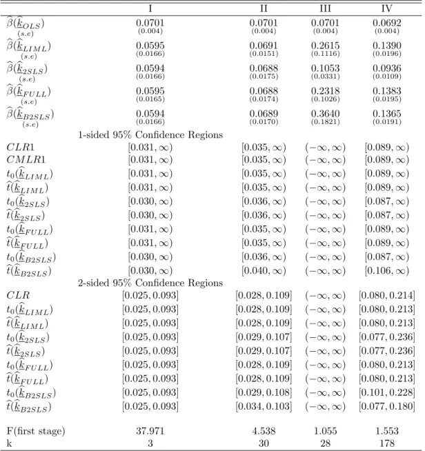
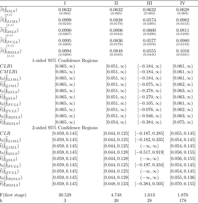
Tables 1 to 3 provide speci…cations for the empirical example. Speci…cations I and II use quarter-of-birth and quarter-of-birth year-of-birth respectively as instruments, and include a constant, race, metropolitan area and marital status, nine year-of-birth and eight regional dummies as controls. Speci…cation III adds
age and age2 as covariates and allows interaction between quarter-of-birth and year-of-birth. Speci…cation
IV replaces year-of-birth dummies used in speci…cation III by state-of-birth dummies.
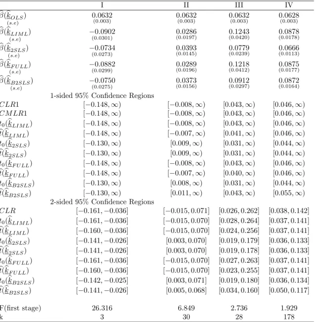
The …rst rows present the OLS, LIML, 2SLS, Fuller and B2SLS estimators with their respective standard errors. We next present 95% con…dence con…dence intervals for one-sided tests: CMLR1 and unbiased t-tests based on the LIML, 2SLS, Fuller and B2SLS estimators. Finally we present 95% con…dence intervals for two-sided tests: CLR and unbiased t-tests based on the LIML, 2SLS, Fuller and B2SLS estimators.
We focus on speci…cation IV, shown byCruz and Moreira(2005) to be informative for returns to schooling despite the low …rst-stage F-statistic and 178 instruments. The LIML estimator is larger than the 2SLS estimator for the three cohorts. We …rst report con…dence intervals for one-sided tests: CMLR1 and the t-tests based on the 2SLS and LIML estimators. One-sided tests may be appropriate in this application. Because returns to schooling are non-negative, we can test against the alternative H1 : > 0(= 0). The
con…dence regions for the t-tests are comparable despite the associated estimates being quite di¤erent. For example, take the 1930-39 cohort. The 2SLS estimates returns to schooling to be 8.1% while the LIML estimate is 9.8%. The lower bound for our con…dence regions is about the same (6.1%-6.3%). In the one-sided case we do not make a statement about the upper bound on returns to schooling.
Next we report con…dence intervals for two-sided tests: the CLR test and unbiased t-tests based on the 2SLS and LIML estimators. As in the one-sided case, con…dence regions for the t-tests and CLR test are comparable. The lower bound for our con…dence regions of the 1930-39 cohort is about the same across two-sided tests (5.4-5.6%), while the upper bound for the unbiased t-tests using the 2SLS estimator is slightly larger than using the LIML estimator (15.5% instead of 14.5%). The unbiased t-tests and the CLR test produce comparable con…dence intervals. In particular, the con…dence regions centered around the 2SLS estimator can be informative even when the …rst-stage F-statistic is low. This empirical exercise supports our theoretical work on the use of the 2SLS and con…dence intervals based on unbiased t-tests in applied work.
Table 1: E¤ects of Years of Education on Log Weekly Earnings (1920-29 cohort) I II III IV b(bkOLS) (s:e) 0:0701 (0:004) 0:0701(0:004) 0:0701(0:004) 0:0692(0:004) b(bkLIM L) (s:e) 0:0595 (0:0166) (0:0151)0:0691 0:2615(0:1116) (0:0196)0:1390 b(bk2SLS) (s:e) 0:0594 (0:0166) (0:0175)0:0688 0:1053(0:0331) (0:0109)0:0936 b(bkF U LL) (s:e) 0:0595 (0:0165) (0:0174)0:0688 0:2318(0:1026) (0:0195)0:1383 b(bkB2SLS) (s:e) 0:0594 (0:0166) (0:0170)0:0689 0:3640(0:1821) (0:0191)0:1365
1-sided 95% Con…dence Regions
CLR1 [0:031; 1) [0:035; 1) ( 1; 1) [0:089; 1) CM LR1 [0:031; 1) [0:035; 1) ( 1; 1) [0:089; 1) t0(bkLIM L) [0:031; 1) [0:035; 1) ( 1; 1) [0:089; 1) bt(bkLIM L) [0:031; 1) [0:035; 1) ( 1; 1) [0:089; 1) t0(bk2SLS) [0:030; 1) [0:036; 1) ( 1; 1) [0:087; 1) bt(bk2SLS) [0:030; 1) [0:036; 1) ( 1; 1) [0:087; 1) t0(bkF U LL) [0:031; 1) [0:035; 1) ( 1; 1) [0:089; 1) bt(bkF U LL) [0:031; 1) [0:035; 1) ( 1; 1) [0:089; 1) t0(bkB2SLS) [0:030; 1) [0:036; 1) ( 1; 1) [0:087; 1) bt(bkB2SLS) [0:030; 1) [0:040; 1) ( 1; 1) [0:106; 1)
2-sided 95% Con…dence Regions
CLR [0:025; 0:093] [0:028; 0:109] ( 1; 1) [0:080; 0:214] t0(bkLIM L) [0:025; 0:093] [0:028; 0:109] ( 1; 1) [0:080; 0:213] bt(bkLIM L) [0:025; 0:093] [0:028; 0:109] ( 1; 1) [0:080; 0:213] t0(bk2SLS) [0:025; 0:093] [0:029; 0:107] ( 1; 1) [0:077; 0:236] bt(bk2SLS) [0:025; 0:093] [0:029; 0:107] ( 1; 1) [0:077; 0:236] t0(bkF U LL) [0:025; 0:093] [0:028; 0:109] ( 1; 1) [0:080; 0:213] bt(bkF U LL) [0:025; 0:093] [0:028; 0:109] ( 1; 1) [0:080; 0:213] t0(bkB2SLS) [0:025; 0:093] [0:029; 0:108] ( 1; 1) [0:101; 0:228] bt(bkB2SLS) [0:025; 0:093] [0:034; 0:103] ( 1; 1) [0:077; 0:180] F(…rst stage) 37.971 4.538 1.055 1.553 k 3 30 28 178
Table 2: E¤ects of Years of Education on Log Weekly Earnings (1930-39 cohort) I II III IV b(bkOLS) (s:e) 0:0632 (0:003) 0:0632(0:003) 0:0632(0:003) 0:0628(0:003) b(bkLIM L) (s:e) 0:0999 (0:0210) (0:0179)0:0838 0:0574(0:0385) 0:0982(0:0153) b(bk2SLS) (s:e) 0:0990 (0:0207) (0:0164)0:0806 0:0600(0:0290) 0:0811(0:0109) b(bkF U LL) (s:e) 0:0995 (0:0209) (0:0178)0:0836 0:0577(0:0378) 0:0980(0:0153) b(bkB2SLS) (s:e) 0:0994 (0:0208) (0:0183)0:0848 0:0555(0:0445) 0:1016(0:0161)
1-sided 95% Con…dence Regions
CLR1 [0:065; 1) [0:051; 1) [ 0:184; 1) [0:061; 1) CM LR1 [0:065; 1) [0:051; 1) [ 0:184; 1) [0:061; 1) t0(bkLIM L) [0:065; 1) [0:051; 1) [ 0:184; 1) [0:061; 1) bt(bkLIM L) [0:065; 1) [0:051; 1) [ 0:075; 1) [0:062; 1) t0(bk2SLS) [0:065; 1) [0:051; 1) [ 0:378; 1) [0:063; 1) bt(bk2SLS) [0:065; 1) [0:051; 1) [ 0:270; 1) [0:063; 1) t0(bkF U LL) [0:065; 1) [0:051; 1) [ 0:105; 1) [0:061; 1) bt(bkF U LL) [0:065; 1) [0:051; 1) [ 0:076; 1) [0:062; 1) t0(bkB2SLS) [0:065; 1) [0:051; 1) [ 0:946; 1) [0:063; 1) bt(bkB2SLS) [0:065; 1) [0:054; 1) [ 0:384; 1) [0:075; 1)
2-sided 95% Con…dence Regions
CLR [0:059; 0:145] [0:044; 0:125] [ 0:187; 0:285] [0:055; 0:145] t0(bkLIM L) [0:059; 0:145] [0:044; 0:125] [ 0:182; 0:335] [0:054; 0:145] bt(bkLIM L) [0:059; 0:145] [0:044; 0:125] ( 1; 1) [0:054; 0:145] t0(bk2SLS) [0:059; 0:145] [0:044; 0:128] [ 0:517; 0:919] [0:056; 0:155] bt(bk2SLS) [0:059; 0:145] [0:044; 0:128] ( 1; 1) [0:056; 0:155] t0(bkF U LL) [0:059; 0:145] [0:044; 0:125] [ 0:197; 0:334] [0:054; 0:145] bt(bkF U LL) [0:059; 0:145] [0:044; 0:125] ( 1; 1) [0:054; 0:145] t0(bkB2SLS) [0:059; 0:145] [0:044; 0:128] ( 1; 1) [0:055; 0:136] bt(bkB2SLS) [0:059; 0:145] [0:048; 0:123] [ 0:384; 0:505] [0:070; 0:155] F(…rst stage) 30.528 4.748 1.613 1.870 k 3 30 28 178