IMPLE AND ROBUST TESTS OF THE QUADRATIC BREAK TREND HYPOTESHIS FOR (0),

(1)

MASTER OF SCIENCE IN

F

INANCE

MASTERS FINAL WORK

DISSERTATION

SIMPLE AND ROBUST TESTS OF THE QUADRATIC BREAK

TREND HYPOTESHIS FOR

𝐼(0)

,

𝐼(1)

AND

𝐼(2)

TIME SERIES.

JOANA MATIAS CORREIA

(2)

M

ASTER OF

S

CIENCE IN

F

INANCE

M

ASTERS

F

INAL

W

ORK

D

ISSERTATION

S

IMPLE AND ROBUST TESTS OF THE QUADRATIC BREAK

TREND HYPOTESHIS FOR

𝐼(0)

,

𝐼(1)

AND

𝐼(2)

TIME SERIES

.

J

OANA

M

ATIAS

C

ORREIA

S

UPERVISOR

:

P

ROF

.

N

UNO

R

ICARDO

M

ARTINS

S

OBREIRA

(3)

`

(4)

Through all these years that I have been a student, only a few number of

teachers were able to share their knowledge and expertise in such a demanding

but humble way as my supervisor did. For this, and for all the enthusiasm,

dedi-cation, and a little bit of patience sometimes, I am sincerely grateful to Professor

Nuno Sobreira.

I am also grateful to ISEG for all the experiences and opportunities that it had

(5)

Esta tese teve como objetivo a construc¸ ˜ao de uma estat´ıstica de teste para

a hip ótese nula da n ão exist ência de quebra na tend ência de uma s érie

tempo-ral unidimensional. A sua principal inovac¸ ˜ao foi o desenvolvimento de um teste

robusto n ão s ó para a presença de erros I(0) e I(1) mas tamb ém para erros

I(2). Para isso, construiu-se um modelo quadr ´atico que incluiu uma vari ´avel

aux-iliar, com a mesma ordem, e foram propostos dois testes distintos, um para uma

data de quebra conhecida e o outro para uma data de quebra desconhecida. O

primeiro ´e uma m ´edia ponderada pelas estat´ısticas de teste apropriadas para o

caso em que os erros s ˜aoI(0), I(1) ou I(2). Esta estat´ıstica de teste tem uma

distribuiç ão normal padr ão. O segundo é uma m édia ponderada que se obt ém

depois de encontrado o supremo sobre todas as poss´ıveis datas de quebra,

su-jeitas a um par ˆametro delimitador da amostra. Neste caso, os valores cr´ıticos

foram calculados atrav és de simulaç ão de Monte Carlo. A metodologia de

Har-vey et al. (2009) foi seguida em ambos os cen ´arios. Mais ainda, conceitos sobre

converg ência assint ótica para processos com duas ra´ızes unit árias foram

revis-tos e algumas propriedades assint ´oticas de regress ˜oes, com uma ou duas ra´ızes

unit árias, foram derivadas. Os testes desenvolvidos t êm aplicaç ão no estudo de

s ´eries econ ´omicas e financeiras.

Palavras-chave:

Quebra estrutural; processo integrado de ordem

(6)

The aim of this thesis was the construction of a test statistic for the null

hy-pothesis of no break in trend in an univariate time series. The breakthrough was

to make the test robust not only for the presence ofI(0)andI(1) shocks but also

for theI(2) case scenario. For this reason, a quadratic trend break model and a

quadratic dummy variable were designed. The assumption of known or unknown

break date motivated the construction of two separate test statistics. The former

is a weighted average of the appropriate t-statistics for the case ofI(0), I(1)and

I(2) shocks and it was shown to have standard normal limiting distribution. The

latter is a weighted average of the statistics formed as the supremum over all

pos-sible break dates, subject to a trimming parameter. In addition, the critical values

for this test statistic were computed through Monte Carlo simulation. The general

framework of Harvey et al. (2009) was adopted to test for the presence of a break

under a known or unknown break date. At the same time, asymptotic theory for

I(2) processes was reviewed and simple asymptotic properties of second and

first order auto-regressions were derived. The tests can be applied to the study

of financial and economic time series.

Keywords:

Structural break; double integrated process; quadratic trend;

(7)

List of Tables

I Asymptotic critical values,mξ1 andmξ2 for thetλ,2 test statistic. . . 26

II Error terms after first and second differences. . . 35

(10)

List of Figures

1 Probability density functions oft∗

0,t∗1 andt∗2. . . 27

2 The Frisch-Waugh-Lovell Theorem withX1 ⊥X2. . . 34

3 Plot of the stochastic functionX∗

(11)

Basic Notation

General

1(A)(x) indicator function; it is equal to1ifxbelongs to the setA

and equal to0, otherwise

⌊x_⌋ integer part of a real numberx

σ standard deviation

µ expected value

N(µ, σ2₎ _{normal distribution with expected value}_µ_{and variance} _σ2

T dimension of the sample

x′ _{transpose of}_x

x:=y xis defined byy

≡ identical to

p

→ convergence in probability

d

→ convergence in distribution

g(n) =o(f(n)) means thatg(n)/f(n)_→0, that is, the functiong(n)is negligible

compared tof(n)

g(n) =O(f(n)) means thatg(n)/f(n)_→c, wherecis a constant; that is,

the functions grow at the same rate

[.]jj denotes thejj′th element of a matrix

[.]j denotes thej′th element of a vector

ξ significance level

(12)

Unit Root Functions

I(d) integrated process of orderd

I(0) stationary process apart from the

deterministic components

I(1) unit root process

I(2) two unit roots process

AR(d) autoregressive process of orderd

DT Qt quadratic dummy variable. D stands for dummy,

T for trend and Q for quadratic

DT Lt linear dummy variable. L stands for linear

DT Ut step dummy variable

△ first differences

△2 _{second differences}

W(r) standard Brownian motion

Acronyms

DGP data generating process

OLS ordinary least squares

LR long run

i.i.d. independent and identically distributed

The symboldenotes the end of a Proof. Each section is divided into

subsec-tions, with consecutive labelling of Equasubsec-tions, Lemmas, Proposisubsec-tions, Remarks

(13)

1 Introduction

Structural changes have been described as a widespread phenomenon in

economics and finance. They are a consequence of a rare but outstanding

his-torical event that changes permanently the behaviour of a standard economic

time series. With no surprise, the existence of such events affects the statistical

properties of estimators, compromising forecasts and statistical inference from

the data. For that reason, the econometric literature has proposed a number of

statistics to test for the presence of structural breaks in a given time series.

In recent years, with an added relevance to this thesis, there has been an

up-surge of interest on devising tests for the breaking trend hypothesis which can be

used regardless of whether the underlying shocks areI(0)orI(1)processes. The

most relevant papers on the subject include Kwiatkowski et al. (1992), Sayginsoy

and Vogelsang (2004), Harvey et al. (2009), Kejriwal and Perron (2010) and

Per-ron and Yabu (2012). Sobreira and Nunes (2015) provided tests of the presence

of multiple breaks in the trend function which are valid in the presence of

station-ary or unit root time series. Apart from the I(0) and I(1) shocks, some studies

found statistical evidence for the presence of two unit roots in prices, wages, stock

variables, among others (see Haldrup, 1998, for example). Therefore, it is

per-fectly viable that some financial and economic time series are better described by

anI(2) process rather than anI(0)or I(1) process. Hence, creating a statistical

procedure that may be used to test the null hypothesis of no breaks in trend which

(14)

of research.

Thus, the purpose of this thesis is to construct a test statistic that can be used

to test the null hypothesis of no break in the trend function against the alternative

hypothesis of one break in the quadratic trend and which is robust as to whether

the underlying shocks are stationary, a random walk or a process with two unit

roots. The first test statistic proposed is valid under the assumption of a known

break date. It is a weighted average of the optimal tests appropriate for theI(0),

I(1) andI(2) shocks. It is proved that the test statistic has standard normal

dis-tribution so that tabulated critical values can be used. The second test statistic is

valid under the assumption of an unknown break date and follows the framework

proposed by Andrews (1993) and Harvey et al. (2009). This hypothesis brings

additional complexity to the testing procedure: the break date must be estimated

through a statistic formed as the over all possible break dates, conditional to a

trimming parameter. The critical values can be calculated through Monte Carlo

simulation.

The outline of this thesis is as follows. Section 2 provides a literature review

on structural changes and unit root hypothesis testing. Sections 3 and 4 establish

the general framework. In section 5, the test statistics for the known and for

the unknown break date are presented. Section 6 illustrates the critical values

computed for the unknown break date test statistic. Section 7 is reserved for

concluding comments and suggestions for future research. Mathematical proofs

are systematized in appendix A and asymptotic theory is summarized in appendix

(15)

2 Literature Review

This thesis is about simple and robust tests for a structural break in the trend

function that includes the case of double integrated shocks in an univariate time

series. For that reason, this literature review covers the most important concepts

and theories related with structural breaks and shocks with two unit roots.

By robust it is meant that testing for the presence of a changing point does

not require to test in advance if the series is stationary, a unit root or a two unit

roots process. This does not mean, though, that we can disregard any information

related with the nature of the shocks. On the contrary, a robust test is one that can

assess several levels of information simultaneously. This type of test procedure

could only be possible after significant discoveries in asymptotic theory as well as

with the introduction of mathematical concepts from calculus, real analysis and

stochastic processes.

Regarding time series with two unit roots, they have been reported as being

rare within the economic and financial context. But how much confidence can be

given to this result when existing unit root test do not even consider the existence

of those time series? Will it be possible to detect more series that mimic anI(2)

process if a test statistic is taken without testinga priori the nature of the shocks?

If this is somehow feasible, it can be extremely useful since researchers are less

likely to make errors while investigating the deterministic or stochastic properties

of the time series under analysis.

(16)

of structural break, shows the most import contributors to the field of structural

break and unit roots testing, with special attention to the works of Perron (1989),

Kwiatkowski et al. (1992) and Harvey et al. (2009). It also explains the interest

of extending existing robust tests to theI(2)case. This literature will not discuss

in detail different approaches to estimate the break date nor multiple break tests

since it is out of the scope of this thesis.

2.1 Structural Break Tests

The concept of structural break has not always been clear in the literature.

Although there is no formal definition of structural break, in what follows it will be

adopted the one of Hansen (2001) which says that “a structural break occurs if at

least one of the parameters of a model changes at some date, the break date, in

the sample period”. In this thesis, the attention will be focused on the curvature

of the trend function given by the quadratic term of the proposed model.

The first studies about structural changes that are considered worth

mention-ing, for the purpose of this thesis, are those of Quandt (1958) and Brown et al.

(1975). Both provided rudimentary tests that were based on parameter instability.

The test developed by Quandt (1958), which became known as the Q statistics,

consisted in a maximization of the likelihood function, at a single known break

date. Another feature of the model was that it only considered normally distributed

disturbances. Nevertheless, the author did not question which parameters were

responsible for a possible switching point nor the consequences of a loss in power

(17)

turn, introduced the Cumulative Sum (CUSUM) statistics to detect instability in the

level of the model and the Cumulative Sum of Least Squares (CUSQ) for testing

error variance instability. Subsequent works of Ploberger and Kr ¨amer (1990) and

Ploberger and Kr ¨amer (1992) applied the CUSUM test to ordinary least squares,

instead of recursive residuals, and showed that the limit distribution under the

null hypothesis of parameter stability could be expressed in terms of Brownian

Bridges. Although innovative for the time, all the aforementioned tests had

rele-vant limitations. Vogelsang (1999), while studying the causes of non monotonic

power functions of standard tests, found that the magnitude of trend shift

exacer-bated the estimated variance of the errors. As a consequence, the power of the

underlying test (extended version of Q and CUSUM statistics) dropped near to

zero.

At the same time, another strand of literature came up with a different but

relevant approach to test the null hypothesis of a unit root in the presence of a

structural break. This major breakthrough in unit root testing in the presence of

a structural break is attributed to Perron (1989). In fact, the author proved that

the presence of a structural change could bias unit root tests, such as Dickey and

Fuller (1979), towards the non rejection of the unit root null hypothesis. To

over-come this issue, Perron suggested that before making any statistical inferences,

the break should be “modelled”, that is, the deterministic component of the time

series should be split into two parts, each one containing the observations before

and after the break. The preselected break dates coincided with relevant

(18)

Price Shocks (1973) and the World Wars were responsible for the occurrence of

breaks in U.S. macroeconomic data.

Surprisingly, with the innovations introduced, the author questioned the

promi-nent idea that most time series had a unit root process. By properly modelling a

break, the author found that important financial and economic time series, such

as those initially studied by Nelson and Plosser (1982) did not have any unit root.

This is an important fact because from this moment on, structural change tests

could not be dissociated from unit root testing.

That paper also highlighted the most prominent ideas about asymptotic

the-ory of the time. Phillips (1986) exploited the concept of spurious regressions by

studying linear regressions with integrated random processes and Phillips (1987)

and Phillips and Perron (1988) proposed new tests for detecting the presence of

a unit root where the models were drawn to discriminate unit root non stationarity

and stationarity about a deterministic trend. Park and Phillips (1989) developed

asymptotic theory of regressions for multivariate linear models that included

inte-grated processes of different orders, nonzero means, drifts, time trends, among

others. All these authors provide mandatory reading for those seeking to

under-stand the mathematics behind unit root testing and asymptotic theory.

Nevertheless, Perron (1989) received a lot of criticism. Christiano (1992)

re-fused to accept the assumption of a known break date. In his opinion, the time of

break should always be estimated in order to obtain a conclusion robust to

sub-jective reasoning and data mining. Another paper that highlighted the importance

(19)

As an example, the author studied a macroeconomic indicator from Spain. The

country joined the EU in 1986. At that time, it was expected that such event would

have an impact on the exports and that a structural break would be observed in

that year. Instead, what was found was that the structural break took place an

year earlier. This raised the question of how Perron’s test would behave if the

break time date was misspecified. The author found that such a small difference

would not entail a loss of power, at least asymptotically. However, for a finite

sample, a loss of power would be observed.

In fact, a huge effort was made to propose powerful structural break tests

which allowed for a structural change at an unknown date. Andrews (1993) and

Andrews and Ploberger (1994) are among the most cited authors in this field.

In particular, Andrews (1993) proposed the Wald, Lagrange Multiplier and

Likeli-hood Ratio tests. The innovation of that paper was to consider parameter

insta-bility which allowed for a time structural change at an unknown date. Andrews

and Ploberger (1994) studied the distributional properties of the break date

es-timates. Vogelsang (1997) proposed a Wald-Type test based on the mean and

exponential statistics of Andrews and Ploberger (1994) and the supremum

statis-tics of Andrews (1993). Bai and Perron (1998) addressed the problem of testing

multiple structural changes.

2.2 Trend Break Tests Robust to I(0) and I(1) Shocks

Standard unit root tests have a key role in structural hypothesis testing. These

(20)

be tested. On one hand, the unit root null hypothesis can be tested. As an

ex-ample, there are the Dickey-Fuller, Augmented Dickey-Fuller and Phillips-Perron

tests. On the other hand, it can be tested the null hypothesis of stationarity.

Kwiatkowski et al. (1992) provided straightforward tests of the null hypothesis of

stationarity against the alternative of a unit root, while allowing for error

autocor-relation.

Nevertheless, as it has already been seen by the Nelson and Plosser (1982)

data, it is not straightforward to determine if a time series has a unit root or not.

As a consequence, the lack of confidence about the output provided by an unit

root test can bias structural change tests. This has motivated Perron and Yabu

(2012) to propose a robust type of structural change test. Another relevant paper

in the field is given to Harvey et al. (2009). The authors were not only interested

in testing or searching for the existence of a structural break but also in how

to do it without pre-testing the nature of the shocks. The tests are a weighted

average of the optimal tests appropriate for theI(0)andI(1)case scenarios. The

weighting function employed was based on the KPSS stationary statistics applied

to the levels and growth rate date (Kwiatkowski et al., 1992). But once more, their

analysis failed to include theI(2)case. However, the work of Harvey et al. (2009)

proved to be useful for a large set of this investigation. Sobreira et al. (2014)

and Sobreira and Nunes (2015) proposed a test for multiple structural changes

in the trend function which did not require pre-specifying whether the underlying

time series (the per capita GDP) wasI(0) orI(1). Sobreira et al. (2014) used the

(21)

path that best describes the behaviour of their real per capita GDP.

This thesis takes one step further and proposes an econometric methodology

to test for the presence of a break in the curvature of the trend function. Another

innovation is that the proposed test statistic is also robust to the presence ofI(2)

shocks in the DGP.

2.3 Shocks with Two Unit Roots

The literature about errors with two unit roots is not extensive. One reason

for that is the belief that most time series are well categorized as stationary or

integrated of order one. Nevertheless, some macroeconomic time series like

prices, wages, stock variables, among others, are potentially integrated of order

two (Haldrup, 1998). Hence, this possibility should be taken into account when

conducting empirical research and it is the reason why this thesis is concerned in

making the testing procedure robust toI(2)-ness.

Time series integrated of order two often look smoother and more slowly

changing than known variables integrated of order one. This can be pointed out

as an argument towards their existence. The reason why researchers care so

much about unit root testing is that the number of unit roots presented in a time

series determines the correct approach to render the series stationary. On one

hand, if the process is a random walk or, equally saying, is a single summation

of shocks, then first differences to the original equation should be taken. On the

other hand, if the time series has two unit roots, equally saying, is a double

(22)

become stationary1_.

The most important works concerned with univariate testing forI(2)are Dickey

and Pantula (1987), Dickey and Fuller (1979) and Haldrup (1998). Asymptotic

theory related with two unit roots can be found in Park and Phillips (1989). Their

findings were essential to give the proof of Proposition B.3 in appendix B.

Dickey and Pantula (1987) showed that the null distribution of traditional

aug-mented Dickey-Fuller tests was affected in the presence of two unit roots, after

observing substantial size distortions. Furthermore, an interesting paper which

has motivated this thesis is Haldrup and Lildholdt (2002). The authors proposed

themselves to test the behaviour of standard unit root tests for a single unit root

when there was evidence that double integrated processes were present in the

data generating process. They examined the robustness of Dickey-Fuller and

Phillips-Perron tests for a unit root and concluded that when the underlying series

was doubly integrated it was likely to give rise to excessive rejection of the unit

root null hypothesis in favour to the explosive alternative because the test statistic

would have a non-similar distribution, caused by the extra unit root.

A further instance for the existence of time series with two unit roots is given

by the work of Sen and Dickey (1987) who suggested that U.S. population is a

plausible candidate for anI(2)variable. Georgoutsos and Kouretas (2004) made

the same observation for some nominal price indices in the context of the

pur-chasing power parity. Banerjee et al. (2001) made anI(2) analysis of Australian

inflation and found that the levels of prices and costs were best characterized as

integrated processes of order two.

(23)

3 Assumptions and Methodology

This thesis followed the general framework of Harvey et al. (2009) who

pro-posed a test statistic to test for the presence of a break in the slope of a linear

trend without knowinga priori if the errors were I(0) or I(1). In spite of being a

central paper to this thesis, the linear model and the overall assumptions did not

provide a comprehensive tool to deal with theI(2)case scenario.

In this context, the first innovation of this thesis was to introduce a quadratic

trend to the general framework. Along with that, a quadratic dummy variable was

designed to model a structural break in the presence of an integrated process

of order two. This prevents the appearance of an impulse dummy variable after

taking two differences to render the time series stationary. The implication of an

impulse dummy variable is that the null hypothesis of no break in trend would be

tested with the information provided from a single observation - an infeasible test

to carry out. On the contrary, the suggested quadratic dummy variable ensues an

indicator function which equals zero before the time break and one afterwards.

Furthermore, the quadratic DGP was expected to bring more flexibility to the

test-ing procedure. As expressed by Harvey et al. (2011), a quadratic model offers a

reasonable degree of local non-linearity in the deterministic trend function,

moti-vating the choice of a polynomial model.

Furthermore, it was assumed throughout this work that there is only one break

(24)

4 The Quadratic Trend Break Model

Consider a time-series_{yt}Tt=1 given by the following trend break data

gener-ating process:

yt=α+βt+

1 2ϑt

2₊_{γDT Q}

t(τ∗) +ut t= 1, . . . , T, (1)

ut = (α1+α2)ut−1−α1α2ut−2+εt u1 =ε1 t= 2, . . . , T. (2)

In equation (1),α is a constant, β is the coefficient of the linear trend and(1/2)ϑ

is the coefficient of the quadratic trend. Furthermore, γ is the coefficient of the

quadratic dummy variableDT Qt(τ∗). The quadratic dummy variable can be

de-fined as follows:

DT Qt(τ∗) :=1(t > Tb∗)

h1

2(t−T

∗

b)2

i

t = 1, . . . , T, (3)

whereT∗

b :=⌊τ∗T⌋is the trend break date which is the integer part of the product

of the break fraction, τ∗ _∈_]0,_1[_{, multiplied by the sample’s size,} _T_{. Concerning}

the existence of a break, only two case scenarios were considered. On the one

hand, there may not exist a break in trend. This is expected to happen whenever

the coefficient γ in equation (1) is zero. This means that the time series is well

described by the equation yt = α+βt+ (1/2)ϑt2+ut for t = 1, . . . , T. In other

words, the coefficientsα, β andϑare constant throughout the sample period. On

the other hand, ifγ in equation (1) is different from zero then a break in trend is

expected to occur. In this case, for the points ranging between[1, T∗

(25)

simply equal toα, the coefficient of the linear trend isβ and the coefficient of the

quadratic trend is (1/2)ϑ. For all points in the time interval [T∗

b + 1, T], the level

changes fromαtoα+(1/2)γ(T∗

b)2, the coefficient of the linear trend changes from

βtoβ₋γT∗

b and the quadratic trend changes from(1/2)ϑto(1/2)(ϑ+γ).

In equation (2), the disturbance term ut, or shock, is assumed to have an

AR(2) representation. The constantsα1 and α2, whereα1, α2 ∈ [0,1], determine

the number of unit roots that the autoregressive polynomial can have. Ifα1 = 0

and _|α2| < 1 or |α1| < 1 and α2 = 0 then ut is stationary. If α1 = 0 and α2 = 1

or α1 = 1 and α2 = 0 then ut is integrated of order one. Finally, if both α1 =

α2 = 1 then ut is integrated of order two2. As a benchmark, we naturally have

thatutis stationary whenα1 =α2 = 0. Regarding the process{εt}, two different

approaches can be taken. The most conservative one assumes the stochastic

process to bei.i.d., that is:

Assumption 4.1.a. The process _{εt} is i.i.d with mean zero and constant

vari-anceσ2

ǫ.

Nevertheless, this is an unrealistic assumption since the structural break tests

are typically applied to series which are highly dependent over time (Kwiatkowski

et al., 1992). For that reason, consider Assumption 1 of Sayginsoy and Vogelsang

(2004), which states a weaker assumption about the errors:

Assumption 4.1.b. The process _{εt} is such that εt = c(L)ηt, where c(L) =

P∞

i=0ciLi, with [c(1)]2 > 0 and Pi∞=0i|ci| < ∞, and where {ηt} is a martingale

difference sequence with unit conditional variance andsup_tE(η4

t)<∞.

(26)

Remark 4.1. Under the conditions of Assumption 4.1.b, the LR variance of _{εt}

is given byω2

ε :=limT→∞T−1E

PT

t=1εt

2

=c(1)2_{. Furthermore, when} _u

tis I(0),

with _|α2| < 1, the LR variance of ut is given by ωu2 := limT→∞T−1E

PT

t=1ut

2

,

such thatω2

u =ωε2/(1−α2)2.

It is the order of integration of the shocks that determines the number of

differ-ences that must be taken to the initial model for it to become stationary. For the

purpose of this thesis, if the time series is stationary then regressions in levels

should be used. If the shocks are a random walk, then the correct approach is to

model the first-differences of equation (1). That is:

∆yt =θ+ϑt+γDT Lt(τ∗) + ∆ut t= 2, . . . , T, (4)

DT Lt(τ∗) :=1(t > Tb∗)(t−Tb∗−1/2) t= 2, . . . , T, (5)

whereθ =β₋(1/2)ϑ is a constant.

In the same fashion, if the shocks have two unit roots then second differences

must be taken to render the series stationary. This is given by the equations:

∆2yt=ϑ+γDT Ut(τ∗) + ∆2ut t = 3, . . . , T, (6)

DT Ut(τ∗) :=

          

0 ift < T∗

b + 1,

0.5 ift=T_b∗+ 1,

1 ift > T∗

b + 1.

(7)

The first and second differences of the quadratic trend break model along with

the dummy variablesDT Qt(τ∗),DT Lt(τ∗)andDT Ut(τ∗)provide the appropriate

(27)

5 Tests for a Break in Trend

The null hypothesis of interest is H0 : γ = 0 against the two sided

alterna-tive HA : γ 6= 0. In contrast with traditional testing procedures, in this thesis it

is not needed to pretest the nature of the shocks. For that reason, the

appropri-ate statistics to test for the presence of a structural break in the quadratic trend

are made robust for the presence of I(0), I(1) and I(2) shocks. Following the

same line of reasoning from Harvey et al. (2009), two different test statistics are

presented, one for the known break date and the other for the unknown break

date.

5.1 Known Break Fraction

The proposed test statistic for the known break fraction hypothesis is a weighted

average of the optimal tests forI(0),I(1)andI(2)shocks. However, to build such

test statistic it is mandatory to find the right weights that allow only one of the

t-tests t0(τ∗), t1(τ∗) or t2(τ∗), defined immediately above, to be chosen in the

end. For the sake of brevity, in this section, it is only presented the t-test for each

optimal case.

Firstly, consider the case scenario where ut in equation (2) is I(0) and

As-sumption 4.1.a holds. The optimal test of H0 againstHA rejects for large values

of the absolute value of the t-ratio appropriated for γ when equation (1) is

(28)

t0(τ∗)

H0

:= ˆγ0(τ

∗₎

r

ˆ σ2

0(τ∗)

h {PT

t=1xDT Q,t(τ∗)xDT Q,t(τ∗)′}−1

i

44

, (8)

ˆ

γ0(τ∗) :=

hn_XT

t=1

xDT Q,t(τ∗)xDT Q,t(τ∗)′

o−1_XT

t=1

xDT Q,t(τ∗)yt

i

4, (9)

withxDT Q,t(τ∗) := {1, t, t2, DT Qt(τ∗)}′, σˆ02(τ∗) := T−1

PT

t=1uˆt(τ∗)2 is the OLS

es-timate of the residual variance anduˆt(τ∗) :=yt−αˆ−βtˆ −ϕtˆ 2−γˆ0(τ∗)DT Qt(τ∗)

andϕ = (1/2)ϑ.

Secondly, admit that ut is I(1). The optimal test of H0 against HA rejects for

large values of the absolute value of the t-ratio appropriated forγ when equation

(1) is estimated via OLS in first differenced form. The optimal test is_|t1(τ∗)|and

t1(τ∗)is given by:

t1(τ∗)

H0

:= γˆ1(τ

∗₎

r

ˆ σ2

1(τ∗)

h {PT

t=2xDT L,t(τ∗)xDT L,t(τ∗)′}−1

i

33

, (10)

ˆ

γ1(τ∗) :=

hn_XT

t=2

xDT L,t(τ∗)xDT L,t(τ∗)′

o−1_XT

t=2

xDT L,t(τ∗)∆yt

i

3, (11)

withxDT L,t(τ∗) := {1, t, DT Lt(τ∗)}′,σˆ12(τ∗) := (T −1)−1

PT

t=2vˆt(τ∗)2 andˆvt(τ∗) :=

∆yt−θˆ−ϑtˆ −γˆ1(τ∗)DT Lt(τ∗).

Finally, if ut is assumed to be I(2) then the appropriate inference method

for testing H0 against HA is to consider the t-ratio test associated with γ when

equation (1) is estimated via OLS in second differenced form. That is _|t2(τ∗)|

(29)

t2(τ∗)

H0

:= γˆ2(τ

∗₎

r

ˆ σ2

2(τ∗)

h {PT

t=3xDT U,t(τ∗)xDT U,t(τ∗)′}−1

i

22

, (12)

ˆ

γ2(τ∗) :=

hn_XT

t=3

xDT U,t(τ∗)xDT U,t(τ∗)′

o−1_XT

t=3

xDT U,t(τ∗)∆2yt

i

2, (13)

withxDT U,t(τ∗) := {1, DT Ut(τ∗)}′, σˆ22(τ∗) := (T −2)−1

PT

t=3ˆkt(τ∗)2 andkˆt(τ∗) :=

∆2_y

t−ϑˆ−γˆ2(τ∗)DT Ut(τ∗).

In order to deal with more general I(0), I(1) and I(2) processes for ut the

OLS estimates of residual variance σˆ2

i(τ∗), for i = 0,1,2, can be replaced by

the corresponding non-parametric long run variance ωˆ2

i(τ∗), for i = 0,1,2. As

pointed out by Kwiatkowski et al. (1992), Assumption 4.1.a can bias conclusions

since most economic and financial time series to which the stationary tests can

be applied are usually time dependent. To this end, the LR variance estimators

for theI(0),I(1)andI(2)are defined as follows:

ˆ

ω2₀(τ∗) := ˆσ2₀(τ∗) + 2

T−1

X

j=1

h(j/l)ˆγj,0(τ∗); ˆγj,0(τ∗) :=T−1

T

X

t=j+1

ˆ

ut(τ∗)ˆut−j(τ∗), (14)

ˆ

ω2₁(τ∗) := ˆσ2₁(τ∗) + 2

T−2

X

j=1

h(j/l)ˆγj,1(τ∗); ˆγj,1(τ∗) := (T−1)−1

T

X

t=j+2

ˆ

vt(τ∗)ˆvt−j(τ∗), (15)

ˆ

ω₂2(τ∗) := ˆσ₂2(τ∗) + 2

T−3

X

j=1

h(j/l)ˆγj,2(τ∗); ˆγj,2(τ∗) := (T −2)−1

T

X

t=j+3

ˆ

kt(τ∗)ˆkt−j(τ∗). (16)

The function h(j/l) is called the Bartlett window and h(j/l) := 1₋j/(l+ 1),

where l is the bandwidth parameter and l = O(T1/4₎_{. In this thesis, the same}

(30)

on, any reference tot0(τ∗), t1(τ∗) or t2(τ∗)will mean that they are based on the

LR variance estimators presented in equations (14), (15) and (16).

The Theorem bellow summarizes the asymptotic behaviour of the _|t0(τ∗)|,

|t1(τ∗)|and|t2(τ∗)|statistics under the presence ofI(0),I(1)andI(2) shocks.

Theorem 5.1. Let the time series process _{yt}be generated according to

equa-tions(1)and (2)and let Assumption 4.1.b hold.

(i) Ifutin(2)isI(0)then: (a)|t0(τ∗)|→ |d L00(r, τ∗)|where

L00(r, τ∗) =

R1

0 RT Q(r, τ∗)dW(r)

q R1

0 RT Q(r, τ∗)2dr

,

(b)_|t1(τ∗)|=Op(l/T)1/2and (c)|t2(τ∗)|=Op(l/T)1/2;

(ii) Ifutin(2)isI(1)then: (a)|t0(τ∗)|=Op(T /l)1/2, (b)|t1(τ∗)|→ |d L11(r, τ∗)|where

L11(r, τ∗) =

R1

0 RT L(r, τ∗)dW(r)

q R1

0 RT L(r, τ∗)2dr

,

and (c)_|t2(τ∗)|=Op(l/T)1/2;

(iii) Ifutin (2)isI(2)then: (a) |t0(τ∗)|=Op(T3/l)1/2, (b)|t1(τ∗)|= Op(T /l)1/2 and (c)

|t2(τ∗)|→ |d L22(r, τ∗)|where

L22(r, τ∗) =

R1

0 RT U(r, τ∗)dW(r)

q R1

0 RT U(r, τ∗)2dr

.

Proof. The proof of items (i.b) and (iii.a) are only valid under a set of conjectures

that require careful examination in the future. The proof of the remaining items

(31)

Here,W(r)is a standard Brownian motion on[0,1]andRT Q(r, τ∗₎_{is the}

con-tinuous time residual from the projection of 1(r > τ∗_)(r ₋_τ∗₎2 _{into the space}

spanned by_{1, r, r2_}_,_{RT L(r, τ}∗₎_{is the residual from a projection of}₁_{(r > τ}∗_)(r₋

τ∗₎_{into the space spanned by}_{_{1, r}_}_and_{RT U}_{(r, τ}∗₎_{is the residual from a}

projec-tion of1(r > τ∗₎_{into the space spanned by}_{₁_}_.

The results in Theorem 5.1 show that t0(τ∗)

d

→ N(0,1) if ut is I(0), t1(τ∗)

d

→

N(0,1) if ut is I(1), while t2(τ∗)

d

→ N(0,1) if ut is I(2). As a consequence, the

appropriate two-sided test can be implemented using critical values from the

stan-dard normal distribution if the time of break is assumed to be known.

Remark 5.1. From part (i) of Theorem 5.1 it can be seen that if ut is I(0) then

|t0(τ∗)| attains the Gaussian distribution asymptotically, while |t1(τ∗)|and |t2(τ∗)|

converges in probability to zero. Similarly, from part (ii) of the same theorem, if

ut is I(1) then |t0(τ∗)|diverges, |t1(τ∗)| attains the Gaussian distribution

asymp-totically while_|t2(τ∗)| converges in probability to zero. Finally, from part (iii), if ut

is I(2) then _|t0(τ∗)| and |t1(τ∗)| diverge, though at a different rate, while |t2(τ∗)|

converges to the Gaussian distribution asymptotically.

From the results above and given that the order of integration ofutis not known

a priori three auxiliary functions are proposed to ensure that the statistic _|t0(τ∗)|

of (8) is selected whenut isI(0),|t1(τ∗)|of (10) is selected when utis I(1)while

|t2(τ∗)|of (12) is selected whenutisI(2), thereby ensuring that the asymptotically

optimal test is chosen in the limit, following the same reasoning from Harvey et al.

(2009). To that end, consider this new test statistic for the presence of a break

in the quadratic trend which is based on a weighted average of _|t0(τ∗)|, |t1(τ∗)|

(32)

process:

t∗_λ,₂ = λ(S0(τ∗), S1(τ∗))× |t0(τ∗)|+ [λ(S1(τ∗), S2(τ∗))−λ(S0(τ∗), S1(τ∗))]× |t1(τ∗)|

+[1₋λ(S1(τ∗), S2(τ∗))]× |t2(τ∗)|. (17)

In (17), let λ : R2 → R be a weight function that can either converge to unity

or zero. For the proposed method to work, the functionλ(S0(τ∗), S1(τ∗)) should

converge to unity whenutisI(0) and to zero whenutisI(1)orI(2). On the other

hand,λ(S1(τ∗), S2(τ∗))should converge to unity whenutisI(0)orI(1)and to zero

when ut is I(2). For that reason it is now necessary to choose the appropriate

auxiliary statisticsSi(τ∗) for i = 0,1,2, and the weight functionsλ(S0(τ∗), S1(τ∗))

andλ(S1(τ∗), S2(τ∗)).

The auxiliary statistics were build based on the stationary LM statistics of

Kwiatkowski et al. (1992). They are calculated from the residuals _{uˆt(τ∗)}Tt=1,

{ˆvt(τ∗)}Tt=2 and{ˆkt(τ∗)}Tt=3, each of each invariant to the values ofα,β andγand

ˆ ω2

i(τ∗)fori= 0,1,2is the long run variance estimator.

S0(τ∗) :=

PT

t=1(

Pt

i=1uˆi(τ∗))2

T2_ω_ˆ2 0(τ∗)

, (18)

S1(τ∗) :=

PT

t=2(

Pt

i=2ˆvi(τ∗))2

(T ₋1)2_ω_ˆ2 1(τ∗)

, (19)

S2(τ∗) :=

PT

t=3(

Pt

i=3kˆi(τ∗))2

(T ₋2)2_ω_ˆ2 2(τ∗)

. (20)

The relevant large sample properties of these three statistics are established in

(33)

Lemma 5.1. Let the conditions of Theorem 5.1 hold:

(i) IfutisI(0)then: (a)S0(τ∗) =Op(1), (b)S1(τ∗) =Op(l/T)and (c)S2(τ∗) =Op(l/T);

(ii) IfutisI(1)then: (a)S0(τ∗) =Op(T /l), (b)S1(τ∗) =Op(1)and (c)S2(τ∗) =Op(l/T);

(iii) If ut is I(2) then: (a) S0(τ∗) = Op(T3/l), (b) S1(τ∗) = Op(T /l) and (c) S2(τ∗) =

Op(1).

Proof. The proof is similar to that of Lemma 1 in Harvey et al. (2009).

The previous Lemma suggests two weight functionsλ:_R2 _→

Rsuch that:

λ(S0(τ∗), S1(τ∗)) := e[−(g1S0(τ

∗₎_S₁₍_τ∗₎₎g2_]

, (21)

λ(S1(τ∗), S2(τ∗)) := e[−(g3S1(τ

∗₎_S₂₍_τ∗₎₎g4_]

, (22)

wheregi for i = 1,2,3,4are positive constants in order to keep the convergence

in the limit. For both functions, the large sample convergence is achieved at an

exponential rate. From Theorem 5.1 and Lemma 5.1 the following corollary can

be stated:

Corollary 5.1. Let the conditions of Theorem 5.1 hold.

(i) If ut is I(0) then (a) λ(S0(τ∗), S1(τ∗))

p

→ 1, (b) λ(S1(τ∗), S2(τ∗))

p

→ 1 and

t∗

λ,2 =|t0(τ∗)|+op(1) d

→N(0,1);

(ii) If ut is I(1) then (a) λ(S0(τ∗), S1(τ∗))

p

→ 0, (b) λ(S1(τ∗), S2(τ∗))

p

→ 1 and

t∗

λ,2 =|t1(τ∗)|+op(1) d

→N(0,1);

(iii) If ut is I(2) then (a) λ(S0(τ∗), S1(τ∗))

p

→ 0, (b) λ(S1(τ∗), S2(τ∗))

p

→ 0 and

t∗

λ,2 =|t2(τ∗)|+op(1) d

(34)

Remark 5.2. The results in Corollary 5.1 show that ifutisI(0)thent∗λ,2 is

asymp-totically equivalent to_|t0(τ∗)|. Equivalently, if ut isI(1) thent∗λ,2 is asymptotically

equivalent to_|t1(τ∗)|. Finally, if ut is I(2) then t∗λ,2 is asymptotically equivalent to

|t2(τ∗)|. That is, t∗λ,2 achieves the appropriate limit distribution independently of

the nature of the shocks.

When the break fraction,τ∗_{, can be arbitrarily chosen it was proved that}_t∗

λ,2

d

→

N(0,1), irrespective of whether the shocks are I(0), I(1) or I(2). To allow that

test to be robust toI(2) shocks, both the auxiliary statistic S2(τ∗)and the weight

functionλ(S1(τ∗), S2(τ∗))had to be created and added to existing robust tests for

theI(0)andI(1)processes, after significant transformations. To move forward for

the unknown break fraction the same methodology was applied though the break

date had to be estimated through a maximization process.

5.2 Unknown Break Fraction

This is the most realistic case scenario. As pointed out by Monta ˜n ´es (1997)

the time of break does not always coincide with the announcement of an

eco-nomic event nor with its realization. It can take place further back in time or

ahead. For that reason, a data dependent algorithm is needed to select the date

after which perceptible changes occur in the quadratic time trend. The same

methodology of Harvey et al. (2009) and Andrews (1993) was followed to

esti-mate the break date for theI(0),I(1)andI(2)shocks.

The appropriate statistics to test for the existence of a break in trend is given

(35)

{|t2(τ)|, τ ∈Λ}whereΛ = [τL, τU], and0< τL< τU <1. The quantitiesτLandτU

will be referred as thelower and upper trimming parameters, respectively.

Fur-thermore, consider the setΛ∗ _:= _{⌊_τ

LT⌋, . . . ,⌊τUT⌋} and the true break fraction

τ∗ _∈_Λ_{. The aforementioned statistics are given by the following set of equations:}

t∗_i := sup

s∈Λ∗ ti s T

fori= 0,1,2andT >0, (23)

with associated breakpoint estimators ofτ∗ _{given by}_τ_ˆ

i := arg sups∈Λ∗ t_i s T for

i = 0,1,2 and T > 0, such that t∗

0 ≡ |t0(ˆτ0)|, t∗1 ≡ |t1(ˆτ1)| and t∗2 ≡ |t2(ˆτ2)|.

Furthermore, the dummy variables in section 5.1 must be redefined. In the case

of unknown break fraction DT Qt(ˆτ0) := 1(t > T0∗)[(1/2)(t−T0∗)2], DT Lt(ˆτ1) :=

1(t > T∗

1)(t−T1∗−1/2)and

DT Ut(ˆτ2) =

                

0 ift < T∗

2,

0.5 ift=T∗ 2,

1 ift > T₂∗,

for allt_∈Λ∗,

whereT∗

0 :=⌊ˆτ0T⌋,T1∗ :=⌊τˆ1T⌋andT2∗ :=⌊τˆ2T⌋. Similar considerations must be

adopted to the stationary statistics of Kwiatkowski et al. (1992).

For the unknown break date case the proposed test statistic is given by:

tλ,2 = λ(S0(ˆτ0), S1(ˆτ1))×t∗0+mξ1[λ(S1(ˆτ1), S2(ˆτ2))−λ(S0(ˆτ0), S1(ˆτ1))]×t

∗ 1

+mξ2[1−λ(S1(ˆτ1), S2(ˆτ2))]×t

∗

2. (24)

withλ(S0(ˆτ0), S1(ˆτ1)) :=e[−(g1S0(ˆτ0)S1(ˆτ1))

g2_]

andλ(S1(ˆτ1), S2(ˆτ2)) :=e[−(g3S1(ˆτ1)S2(ˆτ2))

g4_]

.

(36)

I(1)orτˆ2 ifutisI(2).

The large sample behaviour of thet∗

0, t∗1 and t∗2 statistics must be taken both

under the null hypothesis H0 : γ = 0 and the alternative HA : γ 6= 0, when the

shocksutareI(0),I(1)orI(2). For the null hypothesis, it can be proved that:

Theorem 5.2. Let the time series process _{yt}be generated according to

equa-tions(1)and (2)underH0 :γ = 0and let the conditions of Theorem 5.1 hold.

(i) If ut in (2) is I(0) then: (a) t∗0

d

→ sup_τ_∈Λ_|L00(r, τ∗)|, (b) t∗1 = Op(l/T)1/2 and (c)

t∗

2 =Op(l/T)1/2;

(ii) If ut in (2) is I(1) then: (a) t∗0 = Op(T /l)1/2, (b) t∗1

d

→ sup_τ_∈Λ_|L11(r, τ∗)| and (c)

t∗₂ =Op(l/T)1/2;

(iii) If ut in (2) is I(2) then: (a) t∗0 = Op(T3/l)1/2, (b) t∗1 = Op(T /l)1/2 and (c) t∗2

d

→

sup_τ_∈Λ_|L22(r, τ∗)|.

Proof. The sketch of the proof can be found in the appendix A.

Similarly to Lemma 5.1, the large sample behaviour of the S0(ˆτ0), S1(ˆτ1)and

S2(ˆτ2)statistics can also be stated.

Lemma 5.2. Let the conditions of Theorem 5.1 hold:

(i) IfutisI(0)then: (a)S0(ˆτ0) =Op(1), (b)S1(ˆτ1) =Op(l/T)and (c)S2(ˆτ2) =Op(l/T);

(ii) IfutisI(1)then: (a)S0(ˆτ0) =Op(T /l), (b)S1(ˆτ1) =Op(1)and (c)S2(ˆτ2) =Op(l/T);

(iii) IfutisI(2)then: (a)S0(ˆτ0) =Op(T3/l), (b)S1(ˆτ1) =Op(T /l)and (c)S2(ˆτ2) =Op(1).

By using the same arguments as Harvey et al. (2009), regardless of whether

(37)

converge in probability to zero or one, depending on the nature of the shocks.

These results are summarized in Table III.

Although the following Corollary has not been formally proved, it is expected

to describe with some accuracy the asymptotic null distribution of the statistic in

equation (24), underH0 :γ = 0.

Corollary 5.2. Let the conditions of Theorem 5.1 hold. LetH0 :γ = 0hold. Then:

(i) IfutisI(0): tλ,2 =t∗0 +op(1) d

→sup_τ_∈Λ_|L00(r, τ∗)|;

(ii) IfutisI(1): tλ,2 =mξ1t

∗

1+op(1)→d mξ1supτ∈Λ|L11(r, τ

∗₎_|_;

(iii) IfutisI(2): tλ,2 =mξ2t

∗

2+op(1) d

→mξ2supτ∈Λ|L22(r, τ

∗₎

|.

For a given significance level, ξ, under the null hypothesis H0, the constants

mξ1 and mξ2 can be calculated to ensure that, asymptotically, the critical values

of the mξ1supτ∈Λ|L11(r, τ

∗₎_| _and _m

ξ2supτ∈Λ|L22(r, τ

∗₎_| _{coincide with the critical}

values ofsupτ∈Λ|L00(r, τ∗)|, similarly to Vogelsang (1998).

The consistency rates of the statisticst∗

i fori= 0,1,2under a fixed alternative

of the form HA : γ 6= 0 are hard to obtain and the proof of those results are

out of the scope of this thesis and are left for future investigation. Nevertheless,

it is possible to obtain the asymptotic critical values of the test through Monte

Carlo techniques by simulating the appropriate limiting distribution. The practical

(38)

6 Practical Implementation of the Test Procedures

The asymptotic critical values of the test statistic tλ,2 are provided in Table I,

for ξ = _{0.10,0.05,0.01_}, along with the corresponding values mξ1 and mξ2. This

figure was obtained under the null hypothesis of no break in trend, H0 : γ = 0,

against the two-sided alternative HA : γ 6= 0. A 10% trimming parameter was

used such that τL = 0.10 and τU = 0.90, similarly to Sayginsoy and Vogelsang

(2004). By doing so, the searching range for the occurrence of a structural break

is set to the restricted interval[_⌊τ∗

LT⌋,⌊τU∗T⌋]with length⌊0.8T + 1⌋.

The results were obtained by simulation of the appropriate limiting distribution

with discrete approximations forT = 100 and 10000replications using the rnorm

normal random number generator of R version 0.99.879.

Table I:Asymptotic critical values,mξ1 andmξ2 for thetλ,2test statistic.

ξ Critical value mξ1 mξ2

0.10 2.300 1.086 1.159 0.05 2.695 1.096 1.187 0.01 3.489 1.113 1.181

Source: R output

To implement the test statistic it was also needed to specify the constants

g1,g2, g3 and g4. Different constants can be assigned to these values, however,

and as a rule of thumb, the ones to be picked are those that deliver the best

overall performance after Monte Carlo simulations of the finite sample size and

(39)

0 1 2 3 4

0.0

0.2

0.4

0.6

0.8

1.0

1.2

t value

Probability density function

Legend t0* t1* t2*

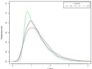
Figure 1: Probability density functions oft∗

0,t∗1 andt∗2.

In this testing procedure, the recommended values of Harvey et al. (2009) were

used such thatg1 = g3 = 500, g2 = g4 = 2 and l = ⌊4(T /100)

1

4⌋. Figure 1 plots

the probability density functions oft∗

0 ,t∗1andt∗2 and it can be observed that for all

cases the asymptotic distribution is skewed to the right.

The source code to apply the test statistictλ,2 to real-life data can be found in

appendix C.

7 Conclusions

This thesis proposed new tests for the presence of a one time structural

change in the trend level of a univariate time series which is valid regardless

of the shocks beingI(0), I(1)or I(2). TheI(2) hypothesis was introduced to the

subject of structural break testing to fulfil a long standing gap in the econometric

literature.

(40)

on the information available about the trend break date. Under a known break

date, the proposed test is a weighted average of the absolute values of three

regression t-ratios, each one appropriate for the case where the data is

gener-ated by an I(0), I(1) or an I(2) process. These statistics were proved to have

standard normal limiting null distributions. For the opposite case scenario, of

un-known break date, additional complexity was brought to the testing procedure. In

fact, asupremum based approach had to be taken to determine the break point

estimators of the true break date. The asymptotic critical values were computed

through Monte Carlo simulation and provided a completely different picture when

compared to the known break date hypothesis.

In the future, it would be useful to restate Theorem 5.1 to a wider scenario.

The results in section 5.2 should also be given more attention. In particular, the

consistency rates of the appropriate statistics under a fixed alternativeHA:γ 6= 0

should be established. Furthermore, size and power tests must be taken for

dif-ferent values of the constants gi for i = 1,2,3,4 to find out which combinations

of values deliver the best overall result. It is also desirable to obtain asymptotic

critical values for50000replications and T = 1000, which requires solving an

op-timization problem while implementing the Monte Carlo simulation. Finally, after

overcoming all these technical issues, it would be interesting to provide tests for

multiple breaks and to propose an empirical application to financial and economic

(41)

References

Andrews, D. W. (1993). Tests for parameter instability and structural change with

unknown change point. Econometrica: Journal of the Econometric Society,

pages 821–856.

Andrews, D. W. and Ploberger, W. (1994). Optimal tests when a nuisance

pa-rameter is present only under the alternative. Econometrica: Journal of the

Econometric Society, pages 1383–1414.

Bai, J. and Perron, P. (1998). Estimating and testing linear models with multiple

structural changes. Econometrica, pages 47–78.

Banerjee, A., Cockerell, L., and Russell, B. (2001). An i (2) analysis of inflation

and the markup. Journal of Applied Econometrics, 16(3):221–240.

Brown, R. L., Durbin, J., and Evans, J. M. (1975). Techniques for testing the

constancy of regression relationships over time. Journal of the Royal Statistical

Society. Series B (Methodological), pages 149–192.

Christiano, L. J. (1992). Searching for a break in gnp. Journal of Business &

Economic Statistics, 10(3):237–250.

Dickey, D. A. and Fuller, W. A. (1979). Distribution of the estimators for

autoregres-sive time series with a unit root. Journal of the American Statistical Association,

74(366a):427–431.

(42)

differenc-ing in autoregressive processes. Journal of Business & Economic Statistics,

5(4):455–461.

Georgoutsos, D. A. and Kouretas, G. P. (2004). A multivariate i (2) cointegration

analysis of german hyperinflation. Applied Financial Economics, 14(1):29–41.

Haldrup, N. (1998). An econometric analysis of i(2) variables. Journal of

Eco-nomic Surveys, 12(5):595–650.

Haldrup, N. and Lildholdt, P. (2002). On the robustness of unit root tests in the

presence of double unit roots. Journal of Time Series Analysis, 23(2):155–171.

Hamilton, J. D. (1994). Time series analysis, volume 2. Princeton University

Press Princeton.

Hansen, B. E. (2001). The new econometrics of structural change: Dating breaks

in us labor productivity. The Journal of Economic Perspectives, 15(4):117–128.

Harvey, D. I., Leybourne, S. J., and Robert Taylor, A. (2011). Testing for unit

roots and the impact of quadratic trends, with an application to relative primary

commodity prices. Econometric Reviews, 30(5):514–547.

Harvey, D. I., Leybourne, S. J., and Taylor, A. R. (2009). Simple, robust, and

pow-erful tests of the breaking trend hypothesis. Econometric Theory, 25(04):995–

1029.

Kejriwal, M. and Perron, P. (2010). A sequential procedure to determine the

num-ber of breaks in trend with an integrated or stationary noise component.Journal

(43)

Kwiatkowski, D., Phillips, P. C., Schmidt, P., and Shin, Y. (1992). Testing the

null hypothesis of stationarity against the alternative of a unit root: How sure

are we that economic time series have a unit root? Journal of Econometrics,

54(1):159–178.

Leybourne, S., Taylor, R., and Kim, T.-H. (2004). An unbiased test for a change

in persistence. Department of Economics Discussion Paper.

Monta ˜n ´es, A. (1997). Level shifts, unit roots and misspecification of the breaking

date. Economics Letters, 54(1):7–13.

Nelson, C. R. and Plosser, C. R. (1982). Trends and random walks in

macroe-conmic time series: some evidence and implications. Journal of Monetary

Economics, 10(2):139–162.

Park, J. Y. and Phillips, P. C. (1989). Statistical inference in regressions with

integrated processes: Part 2. Econometric Theory, 5(01):95–131.

Perron, P. (1989). The great crash, the oil price shock, and the unit root

hypothe-sis. Econometrica: Journal of the Econometric Society, pages 1361–1401.

Perron, P. and Yabu, T. (2012). Testing for shifts in trend with an integrated or

stationary noise component. Journal of Business & Economic Statistics.

Phillips, P. C. (1986). Understanding spurious regressions in econometrics.

Jour-nal of Econometrics, 33(3):311–340.

Phillips, P. C. (1987). Time series regression with a unit root. Econometrica:

(44)

Phillips, P. C. and Perron, P. (1988). Testing for a unit root in time series

regres-sion. Biometrika, 75(2):335–346.

Ploberger, W. and Kr ¨amer, W. (1990). The local power of the cusum and cusum

of squares tests. Econometric Theory, 6(03):335–347.

Ploberger, W. and Kr ¨amer, W. (1992). The cusum test with ols residuals.

Econo-metrica: Journal of the Econometric Society, pages 271–285.

Quandt, R. E. (1958). The estimation of the parameters of a linear regression

system obeying two separate regimes. Journal of the American Statistical

As-sociation, 53(284):873–880.

Sayginsoy, ¨O. and Vogelsang, T. (2004). Powerful tests of structural change that

are robust to strong serial correlation. http://www.albany.edu/economics/

research/workingp/2004/trendbrk.pdf.

Sen, D. and Dickey, D. A. (1987). Symmetric test for second differencing in

uni-variate time series. Journal of Business & Economic Statistics, 5(4):463–473.

Sobreira, N. and Nunes, L. C. (2015). Tests for multiple breaks in the trend with

stationary or integrated shocks. Oxford Bulletin of Economics and Statistics.

Sobreira, N., Nunes, L. C., and Rodrigues, P. M. (2014). Characterizing

eco-nomic growth paths based on new structural change tests. Economic Inquiry,

52(2):845–861.

Vogelsang, T. J. (1997). Wald-type tests for detecting breaks in the trend function

(45)

Vogelsang, T. J. (1998). Trend function hypothesis testing in the presence of serial

correlation. Econometrica, pages 123–148.

Vogelsang, T. J. (1999). Sources of nonmonotonic power when testing for a shift

(46)

A

Mathematical Appendix

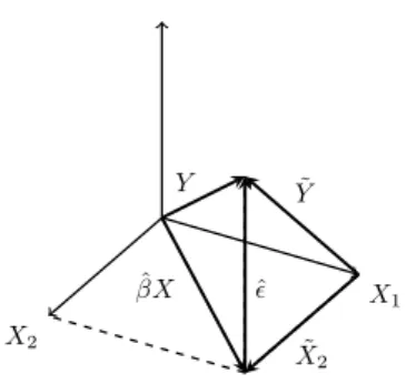
Theorem A.1(Frisch-Waugh-Lovell Theorem (FWLT)). Consider the model Y =

X1β1+X2β2+ε whereX = (X1, X2)andβ = (β1, β2)′. The OLS estimator ofβ2

and the OLS residualsεˆmay be computed by the following algorithm:

1. RegressY onX1; obtain residualsY˜;

2. RegressX2 onX1; obtain residualsX˜2;

3. RegressY˜ onX˜2; obtain OLS estimatesβˆ2 and residualsεˆ.

X2

X1

˜

Y

ˆ

βX Y

˜

X2

ˆ

"

Figure 2: The Frisch-Waugh-Lovell Theorem withX1 ⊥X2.

Proof of Theorem_(5.1)_. _{The proof of this Theorem follows from natural}

exten-sion to Theorem 1 of Harvey et al. (2009) and is done in three steps. First, the

FWLT is applied to estimate γ from equation (1). With this procedure, complex

numerical calculations in inverting high order matrices are avoided. Then, results

about weak convergence from asymptotic theory are applied tot0(τ∗) under the

assumptions that the errors might be eitherI(0), I(1) or I(2). This procedure is

(47)

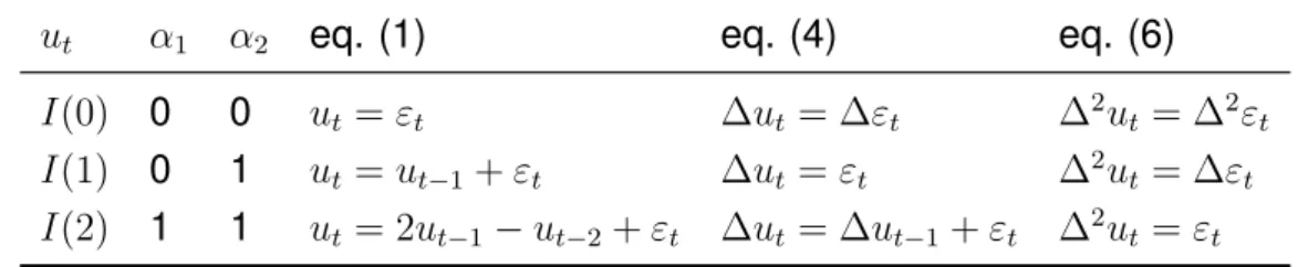
β can be set to zero. Table II bellow illustrates the disturbance term in equations

(1), (4) and (6) under different assumptions about the stationary properties of the

shocks and provides the error terms that appear in the proof of parts I, II and III

below.

Table II:Error terms after first and second differences.

ut α1 α2 eq. (1) eq. (4) eq. (6)

I(0) 0 0 ut=εt ∆ut= ∆εt ∆2ut= ∆2εt

I(1) 0 1 ut=ut−1 +εt ∆ut=εt ∆2ut= ∆εt

I(2) 1 1 ut= 2ut−1−ut−2+εt ∆ut= ∆ut−1+εt ∆2ut=εt

PART I: The regressor γ can be estimated from equation (1) and Theorem

(A.1). To that end, consider equation (25) below:

Yt =γRT Qt(τ∗) +et t= 1, . . . , T, (25)

whereetis an error term,Ytare the OLS residuals from regressingytinto1,tand

t2 _and _{RT Q}

t(τ∗)are the OLS residual from regressingDT Qt(τ∗) into1,t andt2.

It is possible to show that underH0 the test statistict0(τ∗) can be determined by

the following equation:

t0(τ∗) =

PT

t=1RT Qt(τ∗)ut

q

ˆ ω2

0

PT

t=1RT Qt(τ∗)2

. (26)

(i.a) The shocks areI(0): The proof of the weak convergence result is carried

(48)

which states thatωˆ2 0(τ∗)

p

→ω2

u. That is:

t0(τ∗) =

T−5/2PT

t=1RT Qt(τ∗)εt

q

T−5PT

t=1RT Qt(τ∗)2

× p1

ˆ ω2 0 d → R1

0 RT Q(r, τ

∗_)dW_(r)

q R1

0 RT Q(r, τ∗)2dr

,

whereW(r)is a standard Brownian motion on [0,1]and RT Q(r, τ∗₎_{is the}

continuous time residual from the projection of 1(r > τ∗_)(r₋_τ∗₎2 _{into the}

space spanned by_{1, r, r2_}_.

(ii.a) The shocks areI(1): Harvey et al. (2009) extended the results in Kwiatkowski

et al. (1992) to establish the result that (lT)−1_ω_ˆ2 0

d

→ ω2

ε

R1

0 H1(r, τ ∗₎2_dr_,

where H1(r, τ∗)is a continuous time residual from the projection of W(r)

into the space spanned by_{1, r, r2_,₁_{(r > τ}∗_)(r₋_τ∗₎2_}_{. By Proposition B.1,}

items (e), (f) and (g) it can be seen that:

T−7/2Xt2ut = T−7/2

X

t2ut−1 +T−7/2

X

t2εt

= T−7/2Xt2ut−1 +T−5/2T−1

X

t2εt

= T−7/2Xt2ut−1 +

1 TT

−5/2X

t2εt asT → ∞

≡ T−7/2Xt2ut−1 +op(1).

Finally:

(lT−1)1/2t0(τ∗) =

T−7/2PT

t=1RT Qt(τ∗)ut−1

q

T−5PT

t=1RT Qt(τ∗)2

×p 1

(lT)−1_ω2 0

=Op(1).

(iii.a) The shocks are I(2): It can be conjectured from Lemma 5 of Haldrup

and Lildholdt (2002) that (lT)−1_ω2 0

d

→ ω2

ε

R1

0 H2(r, τ

∗₎2_dr_{, where} _H

(49)

a continuous time residual from the projection of W(r) into the space

spanned by _{1, r, r2_,

1(r > τ∗_)(r ₋ _τ∗₎2_}_{. This comes from the fact that}

one more unit root is present in _{ut}. By Proposition B.3, items (j) and

Proposition B.1 item (g) the result follows:

(lT−3)1/2t0(τ∗) =

T−9/2PT

t=1RT Qt(τ∗)ut

q

T−5PT

t=1RT Qt(τ∗)2

× p 1

(lT)−1_ω2 0

=Op(1).

PART II: The regressor γ can be estimated from equation (4) and Theorem

(A.1). To that end, consider following equation:

Yt =γRT Lt(τ∗) +et t = 2, . . . , T, (27)

where et is an error term, Yt are the OLS residuals from regressing ∆yt into 1

andtand RT Lt(τ∗)are the OLS residual from regressing DT Lt(τ∗)into 1andt.

Using the FWLT, it is possible to show that underH0 the test statistic t1(τ∗)can

be determined by the following equation:

t1(τ∗) =

PT

t=2RT Lt(τ∗)∆ut

q

ˆ ω2

1

PT

t=2RT L2t(τ∗)

. (28)

(i.b) The shocks are I(0): It is conjectured that P

RT Lt(τ∗)∆εt ≡ Op(T) and

that lωˆ2 1(τ∗)

p

→ cwhere c = ₋2P∞

s=1sγs′ and γs′ = E(∆ut∆ut−s)(see

Ley-bourne et al., 2004) which implies that:

(T l−1)1/2t1(τ∗) =

T−1PT

t=2RT Lt(τ∗)∆εt

q

T−3PT

t=2RT L2t(τ∗)

× p1

lωˆ2 1

(50)

(ii.b) The shocks areI(1): By Proposition B.1, items (c) and (g) and Remark 4.1

we know thatωˆ1(τ∗)→ω2ε. Finally:

t1(τ∗) =

T−3 2 PT

t=2RT Lt(τ∗)εt

q

T−3PT

t=2RT L2t(τ∗)

×p 1

ˆ ω2

1(τ∗)

d

→ R1

0 RT L(r, τ

∗_)dW_(r)

q R1

0 RT L(r, τ∗)2dr

.

(iii.b) The shocks areI(2):(lT)−1_ω_ˆ2 1 →ωε2

R1

0 H3(r, τ

∗_)dr_{, where}_H

3(r, τ∗)is a

con-tinuous time residual from the projection of W(r) into the space spanned

by _{1, r,1(r > τ∗_)(r ₋_τ∗₎_}_{. According to Proposition B.3 item (g) and}

Proposition B.1 item (g):

(lT−1)1/2t1(τ∗) =

T−5/2PT

t=2RT Lt(τ∗)∆ut

q

T−3PT

t=2RT L2t(τ∗)

×p 1

(lT)−1_ω_ˆ2 1(τ∗)

=Op(1).

PART III: The regressor γ can be estimated from equation (6) and Theorem

(A.1). To that end, consider following equation:

Yt =γRT Ut(τ∗) +et t= 3, . . . , T,

whereetis an error term,Ytare the OLS residuals from regressing∆2ytinto1and

RT Ut(τ∗)are the OLS residuals from regressingDT Ut(τ∗)into1. It is possible to

show that underH0 :γ = 0, equation (12) is equivalent to:

t2(τ∗) =

PT

t=3RT Ut(τ∗)∆2ut

q

ˆ ω2

2

PT

t=3RT Ut2(τ∗)

. (29)

IMPLE AND ROBUST TESTS OF THE QUADRATIC BREAK TREND HYPOTESHIS FOR (0),

MASTER OF SCIENCE IN

F

INANCE

MASTERS FINAL WORK

DISSERTATION

SIMPLE AND ROBUST TESTS OF THE QUADRATIC BREAK

TREND HYPOTESHIS FOR

𝐼(0)

,

𝐼(1)

AND

𝐼(2)

TIME SERIES.

JOANA MATIAS CORREIA

M

ASTER OF

S

CIENCE IN

F

INANCE

M

ASTERS

F

INAL

W

ORK

D

ISSERTATION

S

IMPLE AND ROBUST TESTS OF THE QUADRATIC BREAK

TREND HYPOTESHIS FOR

𝐼(0)

,

𝐼(1)

AND

𝐼(2)

TIME SERIES

.

J

OANA

M

ATIAS

C

ORREIA

S

UPERVISOR

:

P

ROF

.

N

UNO

R

ICARDO

M

ARTINS

S

OBREIRA

Palavras-chave:

Keywords:

Contents

List of Tables

List of Figures

Basic Notation

1

Introduction

2

Literature Review

2.1

Structural Break Tests

2.2

Trend Break Tests Robust to I(0) and I(1) Shocks

2.3

Shocks with Two Unit Roots

3

Assumptions and Methodology

4

The Quadratic Trend Break Model

5