Multi-scale approach using phytoplankton as a first step
towards the definition of the ecological status of reservoirs
Edna Cabecinha
a,*
, Rui Cortes
b, Joa˜o Alexandre Cabral
a, Teresa Ferreira
c,
Martinho Lourenc¸o
d, Miguel Aˆngelo Pardal
eaLaboratory of Applied Ecology, CITAB-Department of Biological and Environmental Engineering,
University of Tra´s-os-Montes e Alto Douro, 5000-911 Vila Real, Portugal
bCITAB-Department of Forestal Engineering, University of Tra´s-os-Montes e Alto Douro, 5000-911 Vila Real, Portugal cCEF-Department of Forestal Engineering, Agronomy Superior Institute, 1349-017 Lisboa, Portugal
d
CGUC-Department of Geology, University of Tra´s-os-Montes e Alto Douro, 5000-911 Vila Real, Portugal
eIMAR (Institute of Marine Research), Department of Zoology, University of Coimbra, 3004-517 Coimbra, Portugal
e c o l o g i c a l i n d i c a t o r s 9 ( 2 0 0 9 ) 2 4 0 – 2 5 5
a r t i c l e
i n f o
Article history:
Received 10 October 2007 Received in revised form 12 April 2008 Accepted 19 April 2008 Keywords: Phytoplankton Ecological status Reservoirs
Water Framework Directive Multivariate analysis Ecological indicators
a b s t r a c t
The growing need to analyse the present state of ecosystems and predict their rate of change has triggered a demand to explore species environment relationships for assessing altera-tions under anthropogenic influence. The Water Framework Directive (WFD) requires the definition of different types of water bodies which are of relevance when assessing their ecological status. The main aim of this study was to define of the types of Portuguese reservoirs located in the North and Centre of Portugal and to assess their ecological status using phytoplankton as water quality indicators. In this study, sampling was carried out in 34 reservoirs during four seasons (spring, summer, autumn and winter), through a period of 8 years (1996–2004).
Two groups of reservoirs could be distinguished, from the multivariate statistical analysis based on environmental variables and on phytoplankton assemblages: G1, lowland reservoirs located in the main rivers (Douro and Tagus), with a very low residence time, characterized by higher water mineral content (hardness and conductivity), higher con-centrations of nutrients (namely, nitrates), dominated by Bacillariophyta and Chlorophyta and characterized by the presence of tolerant of poor environmental conditions species, mainly associated with meso and eutrophic states of water bodies; G2, deeper high altitude reservoirs, largely located in tributaries, with high residence time, presenting a specific species composition under reference conditions, with higher species richness. The transi-tion from deeper and colder reservoirs (reference sites) to shallow and warmer reservoirs (impaired sites), was evident in G2, contrarily to G1, and was mostly positively correlated to organic pollution and mineral gradients. The results presented here are fundamental for the development of a routine for monitoring ecological status according to the WFD.
#2008 Elsevier Ltd. All rights reserved.
* Corresponding author. Tel.: +351 259 350 239; fax: +351 259 350 480. E-mail address:[email protected](E. Cabecinha).
a v a i l a b l e a t w w w . s c i e n c e d i r e c t . c o m
j o u r n a l h o m e p a g e : w w w . e l s e v i e r . c o m / l o c a t e / e c o l i n d
1470-160X/$ – see front matter # 2008 Elsevier Ltd. All rights reserved. doi:10.1016/j.ecolind.2008.04.006
1.
Introduction
Human activity has altered the landscape over centuries, resulting in substantial loss of habitat and aquatic diversity (Young et al., 2005). Broad-scale environmental pressures such as agriculture, point and non point-source pollution, climate change, and land-use change overlap in space and time, requiring that stress measures incorporate assessments of cumulative impacts across multiple stressors (Dziock et al., 2006; Brazner et al., 2007; Danz et al., 2007). Biological assemblages are important sentinels of environmental condi-tions, since they can be more sensitive to the combined effects of stressors than to a single stressor (Karr, 1995; Niemi and McDonald, 2004). Therefore, they integrate cumulative impacts that would not be detected in another way or that would be otherwise underestimated (e.g. habitat degradation, highly variable pollution levels due to point and non-point pollution). Worldwide aquatic ecosystems have been impacted by the excessive release of pollutants, leading to phytoplankton blooms and to the disruption of the structure and functioning of these systems (Robarts, 1985; Reynolds, 1992; Vasconcelos, 2001). The growing need to analyse the present state of ecosystems and to monitor and predict their rate of change, has triggered a demand for studies that explore species environment relationships and use these relationships for assessing and predicting changes under anthropogenic influ-ence (Statzner et al., 2001; Simboura et al., 2005; Ekdahl et al., 2007). The development of indicator systems based on species environment relationships has become a widely used approach for these tasks (Statzner et al., 2001; Dziock et al., 2006). Building on this long tradition of using organisms in monitoring and assessment programs, the European Commission issued a directive mandating the use of different organism groups to monitor the integrity of inland waters and coastal regions. The Water Framework Directive (WFD-2000/60/EC) requires the use of different organism groups such as fish, invertebrates, macrophytes and phytoplankton, either singly or together, in assessing the ecological status of aquatic ecosystems. The WFD takes into account natural variation by proposing that relevant types of surface waters have to be defined first. Their characteristic species composition under reference conditions has to be described. Later on, the assessment of the ecological status shall be achieved by comparing the actual species composition to the one which would be present under undisturbed conditions (so-called reference conditions). How-ever, such claim cannot easily be met, and several restrictions have to be taken into account when defining reference conditions, namely in artificial water bodies. Reservoirs are permanent and artificial lentic water bodies which have been consider as an integrated part of Iberic landscape. In Portugal, these structures are relatively recent and, generally, associated to multiple objectives for human benefits such as supply, irrigation, hydroelectric power and recreation. These water bodies and its biological communities are submitted to enormous spatial–temporal variations, caused by hydric resource use regime. Although Portuguese studies concerning phytoplankton for monitoring water quality are scarce and quite recent (Vasconcelos, 1991, 2001; Boavida and Gliwicz, 1996; Domingues and Galva˜o, 2007), currently, a larger project is underway, led by Portuguese Water Institute (INAG) to establish
ecological status of all Portuguese aquatic systems, involving biological communities including fishes, macroinvertebrates, phytoplankton and macrophytes. Accordingly, the objective of this study was the definition of the different types of all Portuguese reservoirs with hydroelectric power, located in the North and Centre of Portugal. In the present paper, it is discussed the definition of the ecological status and types of reservoirs using phytoplankton as water quality ecological indicators. Based on this, several questions were addressed: what types of reservoirs were identified in the North and Centre of Portugal? How do phytoplankton assemblages and environ-mental variables differ among studied sites? Are landscape scale descriptors related to natural and stressor environment good for defining reference sites? Is phytoplankton community a reliable indicator of the ecological status of artificial water bodies, such as dammed reservoirs?
2.
Materials and methods
2.1. Study areaThis study was carried out in the North and Centre of Portugal in 34 reservoirs from six catchments: Ave (1 reservoir), Ca´vado (6 reservoirs), Mondego (5 reservoirs), and the Portuguese part of the international basins of Lima (2 reservoirs), Douro (11 reservoirs) and Tagus (9 reservoirs) (Fig. 1). The main purpose of all these reservoirs is hydroelectric power, although some secondary uses are also common, such as navigation, irriga-tion, water supply and recreation. Narrow and steep valleys of granite bedrocks morphologically characterize the Northwest of the study area. This region presents a relatively high rainfall average (more than 2200 mm/year) when compared to Mon-dego and Tagus catchments, with a yearly average rainfall of approximately 800 mm/year. The Douro catchment has more than 1400 mm/year in the mountainous northern areas and less than 500 mm/year in the semi-arid central part of this region. In Portugal, although the rainfall presents a high monthly variation, 70% of precipitation occurred between October and April. This extensive geographic area represents a wide range in physical and chemical characteristics, soil use and anthropogenic pressure, including both good and poor water quality conditions. Most of the population lives in the coastal area, and Ave and Ca´vado basins have the largest human population density in Portugal (378 and 265 hab/km2, respectively). Therefore, many impacts associated with urba-nization are present there, namely water quality problems associated with nutrient enrichment and high biochemical oxygen demand (BOD) due to industrial effluent discharges, urban development and intensive agriculture. In contrast, the eastern area of these basins is distinguished by steeper valleys and covered by remnants of native vegetation (the only national park is situated on the upper parts of the Lima and Ca´vado basins). Land use is dominated by agricultural activities in the more western areas. Nevertheless, the Ave basin presents the highest concentration of industry (mainly textile factories), followed by Tagus and Douro basins (mainly transformation industries and mines).
From the initial 38 reservoirs considered in our data set, 4 were removed because of missing environmental data. The e c o l o g i c a l i n d i c a t o r s 9 ( 2 0 0 9 ) 2 4 0 – 2 5 5
241
majority of these reservoirs are explored as true reservoirs (24) (see Table 1), with relatively high residence time and variations along the year, mostly related to seasons. The remaining dammed water bodies (10) are ‘‘run-of-river’’ reservoirs, with very low residence time (days), presenting less stability conditioned by meteorological or hydrological conditions. The main characteristics of the reservoirs are presented inTable 1.
2.2. Environmental parameters and chlorophyll a
From 1996 to 2004, the environmental and biological para-meters were measured by the Laboratory of Environment and Applied Chemistry (LABELEC) four times per sampling year, corresponding to spring (April/May), summer (July/August),
autumn (October/November) and winter (January/February). The sampling periodicity was carried out in a yearly base on 58% of the reservoirs. The remaining reservoirs were visited biannually (26.5%) and triennially (14.7%). This sampling periodicity is also indicated in Table 1. All samples were collected at 100 m from the reservoirs’s crest, at two different depths: (a) near the surface (approximately 0.5 m depth) and (b) near the bottom (2 m above bottom, only for environmental parameters).
Water temperature, turbidity, conductivity, pH and dis-solved oxygen were determined in situ using a YSI handheld multiparameter probe (Yellow Spring Instruments). Light penetration in the water column was determined using Secchi disc method. In the laboratory, major ions, nutrient concentra-tions, BOD5, total silicon, chlorophyll a, faecal coliforms and
Fig. 1 – Location of the 34 reservoirs studied and their distribution through six catchments: Ave, Ca´vado, Mondego, and the Portuguese part of the international basins of Lima, Douro and Tagus.
e c o l o g i c a l i n d i c a t o r s 9 ( 2 0 0 9 ) 2 4 0 – 2 5 5
242
Table 1 – Ranges and median values of important limnological properties of the 34 reservoirs surveyed since 1996–2004
Environmental variables
Code Belver Valeira Picote Carrapatelo Fratel Pocinho Re´gua Miranda Bemposta Crestuma-Lever Vilarinho das Furnas Canic¸ada Lagoa Comprida Salamonde Sta Luzia Touvedo BLV Val PCT CRP FRT PCN RG MRD BMP CRT VILRN CNC¸ LAG SLMD STLZ TVD
Water column variables Epilimnion
Surface water temperature (8C)
Temp 16.8 12.3 16.3 16.5 17.6 14.9 15.6 13.3 15.6 16.8 14.5 15.1 13.1 15.1 18.6 15.7
Turbidity (NTU) Turb 2.96 4.85 4.06 1.69 2.50 4.97 4.26 10.8 1.67 3.13 0.44 1.01 0.84 1.01 1.07 2.68
pH (units) pH 7.82 7.89 8.13 7.82 8.04 8.03 7.78 7.95 8.23 7.70 6.80 6.84 6.48 6.81 6.93 6.83 Dissolved oxygen (mg/L) DO 9.76 9.53 8.61 8.29 10.1 10.8 10.3 9.20 7.98 9.30 9.42 10.1 8.81 10.1 8.63 9.58 Conductivity (mS/cm) Cond 445 327 396 294 413 321 300 416 413 258 15.5 22.3 11.9 21.5 32.1 32.1 Ammonia-N (mg NH4/L) NH4 0.18 0.17 0.13 0.11 0.20 0.15 0.14 0.27 0.18 0.10 0.08 0.09 0.12 0.06 0.12 0.09 Nitrate-N (mg NO3/L) NO3 4.77 6.90 6.24 4.77 4.76 6.05 7.26 7.93 5.33 5.12 0.32 0.64 0.20 0.59 0.87 1.27 Total phosphorus (mg PO4/L) TotP 0.65 0.31 0.34 0.28 0.61 0.29 0.24 0.43 0.38 0.22 0.02 0.04 0.04 0.03 0.04 0.05
Chemical oxygen demand (mg O2/L) COD 12.8 1.40 2.17 8.73 14.1 11.4 11.8 10.7 10.5 7.26 3.01 4.43 3.94 4.79 3.85 6.73 5-day biochemical oxygen demand (mg O2/L) BOD5 1.96 1.84 2.23 1.40 1.61 1.85 1.91 2.07 2.54 1.53 0.66 1.33 0.82 1.16 1.25 1.26 Total silicon (mg SiO2/L) SiO2 5.56 7.28 1.69 3.14 5.92 3.29 4.34 3.15 1.26 3.57 3.59 3.02 1.12 3.80 5.52 3.70
Secchi disk depth (m) SD 1.52 3.39 9.96 2.86 1.86 1.52 2.40 1.23 2.18 1.68 7.09 3.61 5.87 4.10 4.08 2.61
Chlorophyll a (mg/m3) Cpl_a 11.0 0.77 0.99 0.61 12.4 0.76 0.81 0.85 0.89 0.69 0.62 6.27 1.54 2.22 2.46 7.12 Faecal coliform (N/100 mL) FColf 141 31.9 17.9 56.2 337 48.6 40.5 77.2 7.20 29.4 0.89 8.07 0.67 7.81 2.44 9.61 Hypolimnion Water temperature (8C) Temp-Hp 16.41 12.21 14.99 15.92 15.46 13.71 15.13 11.90 11.94 16.37 9.76 11.87 10.15 10.9 12.1 12.9
Turbidity (NTU) Turb-Hp 2.73 6.58 5.79 1.99 3.38 6.36 5.50 20.98 4.60 4.07 0.75 1.72 0.59 2.64 1.98 3.24
pH (units) pH-Hp 7.63 7.85 7.72 7.73 7.52 7.69 7.71 7.85 7.65 7.67 6.53 6.46 6.28 6.34 6.48 6.58 Disolved oxygen (mg O2/L) DO-Hp 8.08 8.03 4.22 6.97 5.60 7.68 8.84 6.20 2.48 8.76 8.23 7.29 8.37 6.07 5.74 6.72 Conductivity (mS/cm) Cond-Hp 451 332 399 301 416 332 304 421 482 262 15.4 22.6 12.2 24.5 31.6 33.69 Total silicon (mg SiO2/L) SiO2-Hp 5.40 3.50 2.58 3.26 6.60 3.58 4.67 3.75 1.89 3.42 3.31 3.83 1.09 3.62 5.98 4.27 Regional variables Altitude (m) Alt 46.15 105 480 71.9 74.0 125 73.5 528 402 13.2 569 162 1600 280 655 50.0 Precipitation (mm) PP 66.49 60.6 53.4 70.2 59.6 58.9 65.5 53.8 53.45 90.4 246 183 160 173 109 204 Catchment area (km2) A 62802 85400 63750 92050 60000 81005 90800 63100 63850 92040 77.0 783 6 642 50.0 1700
Dam area (km2) Dam_A 2.86 7.95 2.44 9.52 7.50 8.29 8.50 1.22 4.05 12.9 3.46 6.89 15.7 2.42 2.46 1.72
Mean dam depth (m) Dp 5.61 11.5 26.9 16.7 17.4 15.6 12.1 31.9 30.8 12.9 34.5 29.5 18.2 31.1 24.3 11.1
Maximum dam depth (m) MxDp 21.00 48.0 100 59.1 43.0 49.0 42.0 80.0 87.0 65.0 94.0 76.0 29.0 75.0 76.0 43.0 Time of residence (days) TimRes 3.39 3.27 5.76 5.24 2.50 2.10 1.45 9.52 2.24 203 38.6 21.7 3.34 Trophic state Mean chlorophyll a (mg/m3) 4 1 1 1 4 1 1 1 1 1 1 3 2 2 3 3 Total phosphorus (mg PO4/m3) TP 5 5 5 5 5 5 5 5 5 5 3 4 4 3 4 4 Secchi disk depth (m) SD 4 3 2 4 4 4 4 5 4 4 2 3 3 3 3 4
Mean annual energy output (GWh)
176 801 1038 870.6 347.5 534 738 1036.3 1086 366.9 225 346 48 232 55 67
Ecological status II II III IV IV IV IV V V V I I I I I I
Use type (regime) a a a a a a a a a a b b b b b b
Sampling periodicity Annual Trianual Annual Trianual Biannual Biannual Trianual Biannual Trianual Annual Biannual Annual Annual Annual Annual Annual Principal watershead Tagus Douro Douro Douro Tagus Douro Douro Douro Douro Douro Ca´vado Ca´vado Mondego Ca´vado Tagus Lima
eco l og ica l indicator s 9 ( 2009 ) 2 4 0 –25 5
243
Environmental variables
Paradela Vale do Rossim
Caldeira˜o Fronhas Alto Lindoso
Alto Rabaga˜o
Venda Nova
Guilhofrei Bouc¸a Poio Torra˜o Cabril Vilar Po´voa Meadas
Pracana Castelo de Bode
Aguieira Varosa Minimum Maximum PRDL V.RSM CLD FRN LND RBG VDNV GUILF BOC¸ POIO TR CBR VLR POV PRCN CBD AG VRS
Water column variables Epilimnion Temperature (8C) 17.3 14.1 17.16 18.01 15.80 16.61 14.80 17.18 16.59 17.25 19.17 18.91 15.80 18.40 20.48 19.16 18.95 16.20 12.31 20.48 Turbidity (NTU) 0.55 0.75 1.54 1.76 1.34 0.83 1.13 1.55 2.11 5.32 2.29 0.99 2.37 4.16 3.02 0.84 1.40 3.16 0.44 10.80 pH (units) 6.88 6.47 7.31 7.66 7.07 6.88 6.83 6.83 7.13 7.97 7.78 7.22 7.74 8.10 8.42 7.38 7.91 7.85 6.47 8.42 DO (mg/L) 8.73 8.76 9.17 9.69 9.43 9.35 9.18 9.57 9.87 10.17 9.29 9.20 9.57 9.49 9.52 9.02 9.21 8.88 7.98 10.76 Conductivity (mS/cm) 18.50 10.35 33.25 45.99 33.07 23.10 23.56 32.42 57.46 99.44 85.36 63.71 55.87 110.01 77.18 71.92 85.26 103.29 10.35 445.00 NH4(mg/L) 0.07 0.07 0.08 0.11 0.08 0.10 0.10 0.08 0.07 0.12 0.11 0.08 0.16 0.28 0.12 0.07 0.10 0.96 0.06 0.96 NO3(mg/L) 0.24 0.10 0.44 0.97 1.07 0.22 0.37 1.57 1.99 0.91 2.60 1.55 0.70 1.51 0.59 1.77 2.04 3.78 0.10 7.93 TotP (mg PO4/L) 0.02 0.04 0.07 0.06 0.04 0.05 0.04 0.05 0.07 0.39 0.10 0.03 0.10 0.34 0.13 0.03 0.08 0.53 0.02 0.65 COD (mg O2/L) 3.96 4.02 6.47 7.28 3.23 5.74 4.57 4.79 4.36 25.59 6.82 4.66 11.19 21.60 10.47 4.08 7.69 13.05 1.40 26.59 BOD5 (mg O2/L) 0.99 0.83 1.35 1.58 1.07 1.05 1.05 1.23 1.43 5.92 1.44 1.00 1.86 2.92 1.47 0.91 1.57 3.38 0.66 5.92 SiO2(mg/L) 4.34 1.91 5.34 5.89 3.66 0.61 2.32 3.48 9.30 3.22 4.94 8.17 2.02 5.09 5.24 4.52 4.81 8.41 0.61 9.30 SD (m) 5.59 5.66 2.73 2.21 5.37 3.57 3.65 2.76 2.65 0.89 2.35 3.98 2.16 1.03 2.34 4.90 2.66 1.54 0.89 7.09 Cpl_a (mg/m3) 1.10 1.80 6.19 8.39 5.79 4.16 3.27 10.42 4.36 31.35 0.77 1.96 1.06 26.97 8.79 1.63 7.84 1.11 0.61 34.58 FColf (N/100 mL) 7.07 5.45 19.10 2.00 6.33 3.69 3.73 12.34 7.91 467.00 49.52 1.20 3.55 49.96 15.57 2.48 6.10 123.00 0.67 467.00 Hypolimnion Temp-Hp (8C) 9.52 11.52 15.60 10.34 11.51 11.53 10.56 14.07 12.42 15.41 15.15 10.98 12.40 14.55 13.66 12.45 14.67 9.54 9.52 16.37 Turb-Hp (NTU) 1.00 1.19 1.87 7.21 3.35 1.23 2.36 2.59 3.52 6.41 2.88 2.94 2.15 5.58 5.31 1.32 2.96 11.65 0.59 20.98 pH-Hp (units) 6.25 6.38 6.91 6.49 6.50 6.55 6.45 6.45 6.59 7.09 6.79 6.69 6.71 6.92 6.89 6.84 6.70 6.67 6.25 7.85 DO-Hp (mg O2/L) 5.82 7.87 6.89 4.26 6.33 6.56 6.45 6.32 5.42 6.04 4.51 3.92 4.92 3.36 3.16 5.40 4.69 1.94 2.48 8.76 Cond-Hp (mS/cm) 17.11 11.80 33.97 63.23 36.41 24.40 23.33 33.34 54.14 102.57 78.40 65.83 56.00 118.07 80.92 68.70 86.19 104.63 11.80 481.90 SiO2-Hp (mg/L) 3.77 2.02 5.90 7.61 4.27 0.72 1.93 4.81 9.58 6.22 6.54 9.19 3.68 7.55 8.22 8.26 7.72 8.45 0.72 9.58 Regional variables Alt (m) 740.00 1436.46 702.00 134.00 338.00 880.00 700.00 335.63 175.00 270.00 65.00 296.00 552.00 311.45 114.00 121.50 124.70 264.00 13.20 1600.00 PP (mm) 164.85 155.14 70.60 114.46 204.26 136.68 161.02 198.88 100.11 66.63 122.72 98.91 79.41 67.27 83.37 99.03 98.27 134.04 53.41 245.97 A (km2) 269 5 32 652 1525 101 356 122 2525 16 3252 2340 370 150 1410 1340 3100 310 4 96303 Mn. dam depth (m) 3.80 0.37 0.66 5.35 10.72 22.10 4.00 16.30 1.85 6.50 20.23 6.70 2.36 5.50 32.91 20.00 0.70 0.37 32.91 Mx. dam depth (m) 42.78 8.91 8.36 19.87 21.44 26.98 24.70 11.58 24.31 8.37 20.74 38.14 15.75 8.55 23.24 33.49 24.86 23.49 5.61 42.78 Dam area (km2) 112.00 27.00 39.00 62.00 110.00 94.00 97.00 49.00 65.00 18.00 70.00 136.00 58.00 32.00 60.00 115.00 89.00 76.00 18.00 136.00 TimRes (days) 196.09 19.20 59.43 108.31 594.12 63.32 7.62 13.52 138.93 320.61 105.43 191.10 50.59 1.45 594.12 Trophic state Mean Cpl_a (mg/m3) 3 2 3 4 3 3 3 4 3 5 1 2 2 5 4 2 3 2 1 5 PO4TOT (mg PO4/m3) 3 4 4 4 4 4 4 4 4 5 4 3 4 5 5 3 4 5 3 5 SD (m) 3 3 4 4 3 3 3 4 4 5 4 3 4 5 5 3 4 4 2 5 AnEng (GWh) 253 28 45 – 948 97 389 11 157.2 4.8 228 301 148 1.6 61.8 390 209.6 60 1.6 1086
Ecological status II II II II II II II III IV IV IV IV IV IV IV V V V
Use type b b b b b b b b b b b b b b b b b b
Sampling periodicity
Biannual Annual Annual Biannual Annual Biannual Annual Annual Biannual Annual Annual Trianual Annual Annual Biannual Annual Annual Annual
Principal watershead
Ca´vado Mondego Mondego Mondego Lima Ca´vado Ca´vado Ave Tagus Tagus Douro Tagus Douro Tagus Tagus Tagus Mondego Douro
(a) ‘‘Run-of river’’ reservoir. (b) Reservoir. Trophic state: 1, ultra-oligotrophic; 2, oligotrophic; 3, mesotrophic; 4, eutrophic; 5, hyper-eutrophic. Ecological status: from I, high status to V, low status.
Table 1 (Continued) ec olo g ical indicato rs 9 ( 2 009) 240–255
244
sulphate reduction bacteria were determined according to methodologies described byAPHA (1995).
To determine the ecological status of the reservoir’s water-sheds, a geographic information system database was created (ESRI, ArcGIS 9.0), with 12 spatial variables. These variables were classified into 4 categories of anthropogenic stress measures that are prominent in the study area: (i) land cover, 6 land use/ land cover variables derived primarily from the Corine Land Cover (CLC, 1990 and 2000) (IGEOE, 2006). Road density (km/ha basin) and proportions for the predominant CLC classes in the basin (urban areas, intensive and extensive agriculture, natural and semi-natural areas and burned areas) were determined; (ii) organic contamination load, 2 variables representing human population pressure (g BOD5/hab eq day by ha basin) and domestic animal pressure (g BOD5/animal eq day by ha basin); (iii) industrial contamination load, 3 variables representing point sources pollution, including number of quarries, mines and transformation industries in the basin (number of sources/ ha basin); and (iv) hydrometric variations, yearly water level changes were determined by the differences between relative average water level and maximum theoretical water level. Points (ii) and (iii) were determined based on data fromINE (2006). A five-score scale was established for all variables (from 1, high status to 5, low status). Therefore, the sum of these five-score scales reflects the final ecological status of the reservoir’s watershed and was classified in the following classes: I, <18; II, 18–22; III, 22–26; IV, 26–30 and V >30. In this study, class I and II were grouped to represent reference reservoirs, and class IV and V were grouped to represent impaired sites.
Although all data characterized anthropogenic stress in some way, there was considerable variation in the types of variables used. Some variables represented the extent of non-natural land cover (e.g. percentage of land devoted to high-intensity residential uses, or to row crops), whereas others represented specific human activities (e.g. point locations of mines) and specific stressors (e.g. hydrometric alterations). All variables were expressed, when possible, on a per-unit area basis.
Trophic classification of reservoirs was obtained from OECD model (Vollenweider and Kerekes, 1982) based on Total phosphorus, Secchi depth and mean chlorophyll a concentra-tion.
2.3. Phytoplankton analysis
Phytoplankton samples were collected from 1996 to 2004, as described for the environmental parameters, using a Van Dorn bottle net, at a depth of approximately 0.5 m. Phytoplankton community composition was studied through inverted micro-scopy, following Utermohl’s method (Lund et al., 1958). For the identification of phytoplankton, samples were fixed in Lugol’s solution (1%, v/v) and, when possible, identified to the species level.
2.4. Statistical analysis
From an initial data set of 710 samples from 1996 to 2004, a subdata set was used for biological and environmental data expressed by means for all sampling years and for each studied reservoir (n = 34). Environmental data were standardized in
order to obtain comparable (dimensionless) scales (Clarke and Warwick, 1994), and variables with more than 10% of data points missing were eliminated. The biological presence/ absence matrix data was transformed in a probability occur-rence matrix (number of presences/number of samples). In this matrix data, rare species (less then three presences in each dam, for all the samples) were omitted from statistical analyses (Forester et al., 2004; Negro and De Hoyos, 2005).
The statistical analysis of the environmental and biological matrices was performed based on multivariate methodologies: (a) for environmental data, a cluster analysis using city-block distances and a discriminant analysis based on Discriminant Canonical Analysis (DCA); (b) for biological data, a cluster analysis trough city-block distances and a comparative analysis based on non-metric multidimensional scaling analysis (n-MDS) and Similarity Percentages-species contributions analysis (SIMPER).
Multivariate analysis (Cluster and DCA) were carried out using STATISTICA1
Version 7 (Stat Soft 2004) and n-MDS and other routines associated were performed using PRIMER1
Version 5.2.2 (Clarke and Gorley, 2001).
Cluster analysis was used to identify natural groupings in the set of data (biological and environmental) without providing any explanation/interpretation. In this study, the similarity measures between sites were based on Ward’s method and City-block (Manhattan) distances. City-block distances measure the distance as the average difference across dimensions. In most cases, this measure yields similar results to the simple Euclidean distance. However in this case, the effect of outliers is dampened (since they are not squared). Afterwards, the matrix of environmental data was ana-lysed by a DCA performed with a forward stepwise method of statistical significance. The DCA was used for detecting the variables that allow discrimination between different (natu-rally occurring) groups.
To compare phytoplankton assemblages and to classify sites along a gradient of human disturbance, a n-MDS and other routines implemented in PRIMER were used. Phyto-plankton population was compared by Bray–Curtis distance calculations using untransformed population data (relative presence for each taxa), and the resulting distance matrix used to infer two-dimensional n-MDS plots.
Statistical differences between clusters identified in n-MDS plots were investigated by a randomization method, ANOSIM (Clarke and Warwick, 1994). This methodology employs R statistics to examine the existence of meaningful differences between the established groups for each considered factor (groups and differences between reference and impaired reservoirs). For each group, a Similarity Percentages-species contributions (SIMPER) was used to determine which species contributed most to the differences among the groups (Clarke and Gorley, 2001), based on the probability of occurrence.
3.
Results
3.1. Environmental variables
The cluster analysis, based on city-block distances, divided the 34 reservoirs into two major groups (Fig. 2). The first cluster e c o l o g i c a l i n d i c a t o r s 9 ( 2 0 0 9 ) 2 4 0 – 2 5 5
245
(G1, Group 1) presents mainly reservoirs (77%) located in the main rivers (Douro and Tagus). These waterbodies are ‘‘run-of-river’’ reservoirs, characterized by having nearly the same inflow and outflow presenting a residence time of 1–4 days. In general, this group represents mainly reservoirs with a trophic state between eutrophic to hyper-eutrophic, mainly due to phosphorus concentration and low transparency (seeTable 1). The second cluster (G2, Group 2) represents reservoirs explored in a true reservoir regime, largely located in tributaries, with a high residence time (weeks to months), and in regions with higher altitudes and mean yearly rainfall. Additionally, these reservoir’s basins present greater slopes and depths than the ones in Group 1 (Table 2). In this cluster it is possible to distinguish two sub-groups: G2.1 consisting of deep and colder water bodies located in the highest altitudes (634.43 m; range: 134–1600 m), precipitation values (yearly mean of 160.34 mm; range: 70–245 mm), slopes (13%; range: 6–22%) and depth (23 m; range: 134–1600 m). Usually, these sites are subject to low anthropogenic stress (see Tables 1 and 2); G2.2 represents shallow and warmer reservoirs subject to higher anthropogenic stress and characterized by lower altitudes (229.37 m; range: 65– 552 m), slopes (9%; range: 4–13%) and precipitation values (yearly mean of 94.98 mm; range: 66–134 mm) (Table 2).
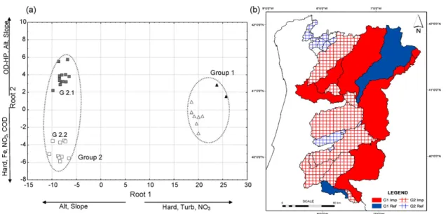
DCA presented very similar result to the cluster analysis. Consequently, the plot of the first two canonical factors (Fig. 3a) allowed to differentiate two major groups and to discriminate between reference and impaired sites within each group. Correlation coefficients among the first two factors and individual environmental variables indicated that Root 1 presented a contrast between hardness/turbidity/NO3
and altitude/slope, whereas Root 2 displayed a contrast between OD-HP/altitude/slope and hardness/NO3/COD.
Multi-variate test statistics (Wilks’ lambda and corresponding
F-value) indicated that there was a significant difference ( p < 0.001) among the cluster centroids for the clusters displayed in Fig. 3a. Univariate F-tests for the individual environmental variables found significant differences among the clusters means for 14 variables from the initial 26.
The first factor explained almost all the variance (92%), and was dominated by hardness (F = 204.06). The second factor accounted only for 7%. Therefore, the ordination graph is consistent with the conclusion that reservoirs from Group 1, ‘‘run-of-river’’ reservoirs, tend to present higher hardness, turbidity and nutrients concentration, namely NO3. In general,
these reservoirs presented watersheds dominated by indus-tries and agriculture that occupied about 50% of the total area (>15% of intensive agriculture).
The separation between reference and impaired sites from Group 2, results mainly from the environmental variables correlated with the second factor. Reference sites from Group 2 were characterized by watersheds with vast natural areas (more than 80%), small agriculture areas (about 16%, but only 3% of intensive agriculture) and good water quality (high DO levels in the hypolimnion. In contrast, impaired reservoirs (G2.2) were subject to higher pollution stress, probably related to watershed soil use, since they were less forested (65%) and presented more agricultural areas (>30%). In Fig. 3b it is possible to see how these reservoirs were spatially clustered. The analysis clearly reflects substantial differences in water chemistry among the two groups of reservoirs defined. InFig. 4, it is possible to observe in all the graphics a pollution gradient (right to left) from Group 2 to Group 1 and from reference to impaired reservoirs based on some environ-mental variables, namely conductivity, hardness, NO3, Cl, SO4
and pH and pH of the hypolimnium (pH-HP). This gradient was again verified in depth (hypolimnion) for the first three Fig. 2 – Classification of sites by Ward’s method based on city-block distance, with environmental data set. The
discontinuous line is the cutting line for defining two reservoirs’s groups and subgroups of Group 1 (G2.1 and G2.2). See Table 1for reservoirs’s abbreviations.
e c o l o g i c a l i n d i c a t o r s 9 ( 2 0 0 9 ) 2 4 0 – 2 5 5
246
variables mention previously. In general, differences among Groups (1 and 2) and among reference versus impaired sites of Group 2, were very significant ( p < 0.001). Contrarily these differences were less obvious between reference versus impaired sites of Group 1. Probably available data set from
reference sites was not large enough to become statistically significant as to determine differences among types. There were a small number of reservoirs of this type (n = 10), and from this group only two sites were selected as best available ones. Only Belver and Valeira reservoirs presented ‘‘good
Table 2 – Median values and standard deviation (S.D.) of important limnological properties of the two groups of reservoirs, and within each group characteristics of reference and impaired sites
ecological status’’ (Class II, seeTable 1) from the score based on anthropogenic stress measures.
3.2. Analysis based on phytoplankton assemblages
From the 710 phytoplankton samples a total of 250 taxa were identified. From these, 55 taxa occurred less then three times in
each reservoir and were excluded from the dataset (see Section 2). The 195 remaining taxa belonged to 7 divisions. Most important in terms of species number and presences were Chlorophyta (75 species, 40.8% of the presences), Bacillariophyta (58 species, 36.4% of the presences) and Cyanophyta (37 species, 10.2% of the presences). There were 9 taxa of Chrysophyta (4.0% of the presences), 5 taxa of Pyrrophyta (2.4% of the presences), Fig. 3 – (a) Discriminant analysis of environmental data relative to cluster structure. Axis interpretation is based on correlation between each variable and the first two discriminant factors. (b) Spatial distribution of the defined reservoirs’s groups. Filled (blue) and empty symbols (red) represent reference and impaired reservoirs, respectively. (For interpretation of the references to color in this figure legend, the reader is referred to the web version of the article.)
Fig. 4 – Differences in some environmental variables concentrations, from epi- and hypolimnion, in the two groups of reservoirs and within each group, in reference (blue) and impaired (red) sites. Box and Whisker diagrams show median, range and 25th and 75th percentiles of values for samples in each group. (For interpretation of the references to color in this figure legend, the reader is referred to the web version of the article.)
e c o l o g i c a l i n d i c a t o r s 9 ( 2 0 0 9 ) 2 4 0 – 2 5 5
248
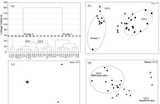
and 3 taxa of Cryptophyta (3.8% of the presences) as well as of Euglenophyta (2.4% of the presences). The cluster analysis of phytoplankton assemblages data, identified in general, the same two major groups as the environmental data (Fig. 5a). The patterns revealed by cluster analysis were apparent in the Non-metric MDS ordination. The n-MDS based on species/site data for all reservoirs (n = 34) was able to differentiate between the two identified groups (stress value of 0.11 for 2D and 0.07 for 3D) (Fig. 5b). Additionally, this analysis was able to distinguish between undisturbed and impaired sites within Group 2 (stress value of 0.12 for 2D and 0.07 for 3D) (Fig. 5d). For Group 1, these differences are not so obvious (stress value of 0.01 for 2D and 3D) (Fig. 5c). In general, the n-MDS analysis displayed a gradient
of disturbance, allowing the scattering of sites along a magnitude range of human impact.
These results were confirmed by the pairwise analysis of similarity (ANOSIM) and SIMPER tests (seeTable 3). The Global ANOSIM test showed that there were significant differences ( p < 0.001) in assemblage composition between the two groups and among reference and impaired reservoirs for all data sets (n = 34) and for Group 2 (seeTable 3). The global R-value is a useful comparative measure of the degree of separation of the groups used (Clarke and Warwick, 1994). In this case, only in data from Group 1 it was not possible to distinguish between reference and impaired groups with a global R (0.351, p = 0.194).
Table 3 – Percentage breakdown of average dissimilarity between groups of reservoirs, and groups of impaired vs. reference sites for all reservoirs with hydroelectric power in Portugal, using SIMPER analysis
Factors Groups Average similarity (%) Average disimilarity (%) Anosim
Groups (n = 34) 1 53.14 71.30 Global R = 0.494***
2 39.83
Ref/Imp (n = 34) Reference 39.86 68.96 Global R = 0.381***
Impaired 41.87
Group 1 (n = 10) Reference 29.66 55.30 Global R = 0.351 (n.s.)
Impaired 54.44
Group 2 (n = 24) Reference 46.80 65.35 Global R = 0.380***
Impaired 40.47
Global R-values for the pairwise analysis of similarity (ANOSIM) tests. Only p < 0.001 (***) was regarded as significant.
Fig. 5 – (a) Site dendrogram and (b) non-metric multidimensional scaling (n-MDS) ordination for 34 Portuguese reservoirs, based on phytoplankton assemblage data. (c) n-MDS for Group 1 and (d) Group 2, respectively. Dotted lines indicate reservoir groups produced by cluster analysis. Circles and triangles represent reference and impaired reservoirs, respectively.
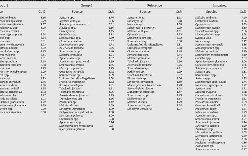
The results of SIMPER analysis that compared groups and reference versus impaired sites (Table 3) are in evident agreement with the patterns observed in the previous analyses. The average dissimilarity between groups was 71.30%, making clear the existence of a strong variability among them. A total of 108 taxa (57.14% of the total taxa) accounted for 90% of the dissimilarity between these two groups. A value of 68.96 and 65.35% of dissimilarity between the most and least disturbed sites (for all reservoirs and within Group 2, respectively) corroborates the hypothesis that these groups are truly different. The most characteristic phyto-plankton taxa of these groups are presented inTable 4(to a cumulative percentage of 75%). From each specific taxa composition it is possible to see that even though both groups were visibly dominated by Bacillariophyta and Chlorophyta they only had six taxon in common: Melosira ambigua, Trachelomonas spp., Scenedesmus ecornis, Monoraphidium spp., Cyclotella spp. and Closterium acutum.
In Group 1, there were not obvious differences among species composition between reference and impaired sites. Indeed, from the 19 most characteristic taxa from reference sites in this group, 10 are present in impaired sites as well. This corroborates the results from Cluster and ANOSIM analysis. Both sites were clearly dominated by Bacillariophyta and Chlorophyta and characterized by the presence of tolerant species, mainly associated from meso to eutrophic states of water bodies. Therefore, meso-eutraphentic species (Van Dam et al., 1994; Tavassi et al., 2004), like Navicula rhynchocephala, Melosira granulata, Synedra pulchella, Pediastrum simplex and Pediastrum duplex, dominated the less disturbed sites from Group 1. Additionally, impaired sites presented eutraphentic species, namely M. ambigua, Cyclotella meneghiana, Synedra ulna, S. pulchella, Nitzschia accicularis and Cocconeis placentala, asso-ciated with blue-green algae, Aphanizomenon flos-aquae and Oscillatoria planctonica.
Reference sites from Group 2 were typified by the intolerant (oligotraphentic to oligo-mesotraphentic) species, Melosira distans, Melosira italica, Tabellaria floculosa, Tabellaria fenestrata and Rhizosolenia eriensis and some mesotraphentic species like Syneda acus. Additionally, in these reservoirs, Chrysophyta, that is known to decrease with disturbance increase, had a significant importance (11.68% versus 1.09% in the impaired sites).
Contrarily, disturbed sites were characterized mostly by tolerant species of several divisions such as Chlorophyta, Bacillariophyta, and Cyanophyta. The present blue-green algae belonged mostly to genera whose ability to produce toxins that can affect a variety of organisms, including humans is known, like Aphanizomenon flos-aquae, Anabaena spp., Microcystis aeruginosa, Microcystis pulverea and Microcystis flos-aquae (Vasconcelos, 1999, 2001; Dokulil and Teubner, 2000; de Figueiredo et al., 2006).
4.
Discussion
Multivariate analyses based on environmental variables and phytoplankton assemblages, allowed to define the different types of surface waters from North and Centre of Portugal. From the studied 34 reservoirs, it was possible to identified and
delimit two types of dammed water bodies which were characterized by different hydromorphological features, water chemistry characteristics and by a specific species composition. Group 1 had mostly ‘‘run-of river’’ reservoirs located in the main rivers (Douro and Tagus), with very small residence time; Group 2 was represented by deeper dammed water bodies with higher residence time, largely located in tributaries, in regions with higher altitudes and average yearly rainfall. In general, Group 1 represented reservoirs with a trophic state between eutrophic to hyper-eutrophic, mainly due to phosphorus concentration and low transparency. Since all these reservoirs belong to International river basins, the trophic state observed may be a consequence of the great anthropogenic pressures that characterized such basins, namely due to upstream intensive agriculture practiced in Spain. The differences in retention time and water depth have a large impact on how eutrophication manifests. According the Vollenweider models, lakes with a high retention time (generally the deeper lakes) will have a lower nutrient concentration than the lakes with a very low retention time (generally the shallower ones) (GIG, 2007).
In general, median Secchi depth, total phosphorus and chlorophyll a concentration were comparable with those reported in previous surveys (Boavida and Marques, 1996) and confirmed the hyper-eutrophic status of the majority of the reservoirs from G1. G2 reservoirs were quite variable, displaying a clear disturbance gradient, with deep colder sites, mainly oligotrophic, while warmer sites showed higher values, mostly eutrophic and hyper-eutrophic status (Boavida and Marques, 1996). Therefore, in this study, it was possible to identify distinct gradients of human disturbance, along which environmental variables and phytoplankton assemblages changed within both reservoirs types.
Among the 26 environmental variables used in multivariate analysis, nitrate concentration and water mineral content were mainly responsible for the dissimilarity among these two groups (Fig. 3). The transition observed inFig. 4, from impaired reservoirs of Group 1 to reference reservoirs of Group 2, reflects substantial differences in water chemistry between the two Groups defined and within reference versus impaired sites. These chemical properties of the water body, originated from geological characteristics of the watershed, seem to assume major importance. The results presented here are consistent with several studies developed in rivers (Stevenson, 1997; Wetzel, 2001) as well as in lakes and reservoirs (Wetzel, 2001; de Figueiredo et al., 2006; Tolotti et al., 2006), who proposed geological properties as an ultimate variable that determines the composition of aquatic community assemblages on a larger spatial scale. However, at a smaller scale, physical character-istics (e.g. reservoir size, temperature/elevation) and human-influenced water quality gradients (e.g. nutrients, BOD5, COD,
turbidity) were more important. The same results were obtained along spatial and environmental gradients at a larger-scale, based on diatom assemblages (Lim et al., 2007); macroinvertebrates, macrophytes and fishes (INAG, 2006).
The typology identified in hydroelectric Portuguese reser-voirs and that was based on environmental variables was also corroborated by changes in phytoplankton assemblage.
This study has identified distinct gradients along which phytoplankton assemblage structure changes within north e c o l o g i c a l i n d i c a t o r s 9 ( 2 0 0 9 ) 2 4 0 – 2 5 5
Table 4 – Average contribution (Ct.%) of species mainly responsible for intra-group similarities
(a) Group 1 Group 2 Reference Impaired
Species Ct.% Species Ct.% Species Ct.% Species Ct.%
Melosira ambigua 5.60 Synedra spp. 6.76 Synedra accus 6.93 Melosira ambigua 7.20
Scenedesmus opoliensis 5.29 Melosira ambigua 5.36 Dinobryon sp. 6.18 Closterium acutum 3.86
Cyclotella meneghiniana 4.37 Sphaerocystis schroeteri 5.31 Navicula spp. 4.68 Cyclotella spp. 3.39
Trachelomonas spp. 3.90 Navicula spp. 4.86 Sphaerocystis schroeteri 4.29 Scenedesmus ecornis 3.30
Scenedesmus ecornis 3.81 Dinobryon sp. 4.45 Melosira ambigua 4.11 Trachelomonas spp. 3.06
Navicula cryptocephala 3.68 Cyclotella spp. 3.82 Cyclotella spp. 3.55 Monoraphidium spp. 2.68
Oocystis spp. 3.64 Scenedesmus spp. 3.69 Monoraphidium spp. 3.12 Synedra ulna 3.02
Synedra ulna 3.51 Closterium acutum 3.67 Scenedesmus spp. 3.00 Navicula spp. 2.42
Navicula rhynchocephala 3.23 Monoraphidium spp. 2.71 Unidentified dinoflagellates 2.81 Scenedesmus opoliensis 2.36
Pediastrum simplex 3.02 Asterionella formosa 2.55 Crucigenia tetrapedia 2.58 Monoraphidium spp. 2.36
Monoraphidium spp. 2.93 Staurastrum spp. 2.40 Closterium acutum 2.48 Melosira granulata 2.29
Diatoma vulgaris 2.81 Melosira granulata 1.91 Aphanothece spp. 2.44 Staurastrum messikommeri 2.10
Pandorina morum 2.51 Aphanothece spp. 1.87 Melosira granulata 2.37 Oocystisspp. 2.07
Melosira granulata 2.45 Scenedesmus quadricauda 1.59 Tabellaria floculosa 2.30 Aphanizomenon flos-aquae 2.04
Micractinium pusillum 2.38 Scenedesmus ecornis 1.55 Asterionella formosa 2.26 Cyclotella meneghiniana 1.86
Synedra acus 2.29 Microcystis pulverea 1.45 Stauradesmus sp. 2.21 Sphaerocystis schroeteri 1.82
Staurastrum messikommeri 2.09 Crucigenia tetrapedia 1.42 Peridinium sp. 2.19 Synedra spp. 1.81
Ankyra spp. 1.97 Stauradesmus sp. 1.39 Tabellaria fenestrata 2.07 Staurastrum spp. 1.81
Cyclotella spp. 1.93 Unidentified dinoflagellates 1.34 Rhizosolenia sp. 2.06 Ankyra spp. 1.75
Pediastrum boryanum 1.76 Fragilaria crotonensis 1.32 Dinobryon bavaricum 1.89 Scenedesmus quadricauda 1.74
Closterium acutum 1.66 Schroederia setigera 1.31 Monoraphidium komarkovae 1.79 Navicula cryptocephala 1.72
Scenedesmus smithii 1.55 Tabellaria floculosa 1.31 Spondylosium planum 1.78 Synedra acus 1.71
Oscillatoria planctonica 1.33 Tabellaria fenestrata 1.25 Elakatothrix gelatinosa 1.47 Diatoma vulgaris 1.58
Pediastrum duplex 1.27 Ankistrodesmus falcatus 1.19 Staurastrum spp. 1.43 Coelastrum reticulatum 1.56
Nitzschia acicularis 1.23 Trachelomonas spp. 1.16 Mallomonas sp. 1.34 Fragilaria crotonensis 1.53
Actinastrum gracillimum 1.22 Peridinium sp. 1.12 Melosira distans 1.29 Pediastrum simplex 1.53
Aphanizomenon flos-aquae 1.19 Melosira distans 1.09 Scenedesmus ecornis 1.18 Ceratium hirundinella 1.52
Closterium spp. 0.99 Dinobryon bavaricum 1.09 Dinobryon sertularia 1.07 Pediastrum duplex 1.31
Scenedesmus arcuatus 0.98 Dictyosphaerium pulchellum 1.00 Nitzschia acicularis 1.29
Microcystis pulverea 1.00 Scenedesmus spp. 1.28
Cosmarium spp. 0.98 Scenedesmus smithii 1.24
Aphanocapsa spp. 0.96 Asterionella formosa 1.24
Monoraphidium komarkovae 0.95 Schroederia setigera 1.20
Spondylosium planum 0.88 Anabaena spp. 1.10
Micractinium pusillum 1.05 Microcystis aeruginosa 0.89 Microcystis pulverea 0.86 Navicula rhynchocephala 0.86 Achnanthes sp. 0.77 Scenedesmus acutus 0.77 eco l og ica l indicator s 9 ( 2009 ) 2 4 0 –25 5
251
(b)
(Group 1) (Group 2)
Reference Impaired Reference Impaired
Species Ct.% Species Ct.% Species Ct.% Species Ct.%
Scenedesmus opoliensis 11.32 Melosira ambigua 6.08 Synedra accus 7.89 Melosira ambigua 9.76
Navicula rhynchocephala 11.32 Cyclotella meneghiniana 4.95 Dinobryon sp. 7.01 Closterium acutum 5.25
Pandorina morum 7.55 Trachelomonas spp. 4.62 Sphaerocystis schroeteri 4.92 Sphaerocystis schroeteri 4.20
Oocystis spp. 4.4 Scenedesmus opoliensis 4.42 Navicula spp. 4.88 Synedra spp. 3.86
Melosira granulata 4.4 Navicula cryptocephala 3.89 Melosira distans 3.74 Navicula spp. 3.54
Staurastrum sebaldi 3.77 Synedra ulna 3.66 Stauradesmus sp. 3.44 Cyclotella meneghiniana 3.44
Scenedesmus ecornis 3.77 Scenedesmus ecornis 3.52 Unidentified dinoflagellates 3.22 Ceratium hirundinella 3.24
Pediastrum boryanum 3.77 Oocystis spp. 3.45 Cyclotella spp. 3.20 Staurastrum spp. 3.17
Actinastrum hantzschii 3.77 Diatoma vulgaris 3.03 Crucigenia tetrapedia 2.96 Fragilaria crotonensis 2.91
Pediastrum simplex 3.14 Pediastrum simplex 3.02 Monoraphidium spp. 2.79 Scenedesmus spp. 2.49
Synedra acus 3.14 Monoraphidium spp. 2.97 Tabellaria floculosa 2.57 Schroederia setigera 2.44
Monoraphidium spp. 2.52 Cyclotella spp. 2.52 Scenedesmus spp. 2.54 Scenedesmus ecornis 2.44
Pediastrum duplex 1.89 Micractinium pusillum 2.46 Asterionella formosa 2.53 Asterionella formosa 2.34
Monoraphidium komarkovae 1.89 Navicula rhynchocephala 3.38 Closterium acutum 2.50 Synedra ulna 2.03
Closterium spp. 1.89 Melosira granulata 2.27 Peridinium sp. 2.44 Scenedesmus quadricauda 2.02
Synedra utermohlii 1.89 Staurastrum messikommeri 2.18 Aphanothece spp. 2.37 Coelastrum reticulatum 2.01
Ankistrodesmus gracilis 1.89 Synedra pulchella 2.05 Dinobryon bavaricum 2.17 Aphanizomenon flos-aquae 1.93
Rhizosolenia sp. 1.89 Ankyra spp. 1.95 Tabellaria fenestrata 2.08 Trachelomonas spp. 1.78
Synedra pulchella 1.89 Pandorina morum 1.92 Melosira italica 1.92 Melosira granulata 1.78
Closterium acutum 1.78 Spondylosium planum 1.82 Monoraphidium spp. 1.69
Nitzschia acicularis 1.77 Rhizosolenia sp. 1.73 Staurastrum messikommeri 1.65
Aphanizomenon flos-aquae 1.70 Elakatothrix gelatinosa 1.60 Ankyra spp. 1.47
Scenedesmus smithii 1.59 Monoraphidium komarkovae 1.53 Oocystis spp. 1.37
Pediastrum boryanum 1.24 Staurastrum spp. 1.36 Pediastrum duplex 1.29
Actinastrum gracillimum 1.16 Mallomonas sp. 1.27 Anabaena spp. 1.24
Oscillatoria planctonica 1.14 Dinobryon sertularia 1.23 Scenedesmus acutus 1.22
Scenedesmus arcuatus 1.10 Microcystis aeruginosa 1.20
Scenedesmus quadricauda 1.10 Ankistrodesmus falcatus 1.19
Cocconeis placentula 1.00 Microcystis pulverea 1.10
Dinobryon sp. 1.09 Microcystis flos-aquae 0.98 Aphanothece spp. 0.91 Nitzschia acicularis 0.90 Table 4 (Continued) ec olo g ical indicato rs 9 ( 2 009) 240–255
252
and centre Portuguese basins. The differences detected among reservoir phytoplankton indicated that species compositions were structured by factors related to geographic location, reservoir type and anthropogenic pressure.
Phytoplankton reacted to various environmental influ-ences and therefore can be used as ecological indicator organisms. However, careful analysis is necessary to distin-guish between effects of natural variability and anthropogenic disturbances. Some authors (Sabater and Nolla, 1991; Negro and De Hoyos, 2005) reported that phytoplankton distribution (namely diatoms) in Spanish reservoirs were influenced by both basin geology and land use. Likewise, phytoplankton assemblages in Canadian and Greek rivers were influenced by a combination of natural and anthropogenic factors ( Cum-ming et al., 1995; Temponeras et al., 2000; respectively). Given the fact, that the studied reservoirs are mainly used for hydroelectric power, must not be disregarded the effects of fluctuations in water level or discharge on species composi-tion, directly related to the management of reservoirs, since these water bodies and its biological communities are submitted to enormous spatial–temporal variations, caused by hydric resource use regime (GIG, 2007).
The phytoplankton of many lakes, especially those of higher trophic levels, is dominated by large, colony forming species of cyanobacteria such as the referenced above. Permanent cyanobacterial dominance is, therefore, regarded as the ultimate phase of eutrophication occurring world-wide (e.g.Robarts, 1985; Pizzolon et al., 1999; Dokulil and Teubner, 2000). Excessive abundance or ‘blooming’ of cyanobacteria generally has detrimental effects on the domestic, industrial and recreational uses of water bodies and is in many cases a direct motivation for restoration measures (Dokulil and Teubner, 2000).
There has been extensive theoretical and empirical work done on the characterization of stressor gradients in the freshwater ecosystem context (Barbour et al., 1999; Brown and Vivas, 2005; Danz et al., 2007). Therefore, followingBailey et al. (2007)criteria, our methodology becomes more comprehen-sive and objective and can allow more powerful, objective bioassessments, since: (1) quantifies all human activities (e.g. agriculture, mining, urban development) that could poten-tially affect the aquatic ecosystem, at multiple scales includ-ing the reservoir and its drainage basin; (2) does not include explicitly the effects of human activity on the aquatic ecosystem; (3) expresses human activity in scale-independent units (e.g. road density in m ha, % basin with intense agriculture) allowing to compare the relationships determined from reservoir water column to larger cumulative effects contexts.
Reservoirs are artificial or heavily modified water bodies (AWB or HMWB). For HMWB and AWB, the reference conditions on which status classification is based are within the range of ‘‘Maximum Ecological Potential’’ (MEP). The MEP represents the maximum ecological quality that could be achieved for these systems, once all mitigation measures that do not have significant adverse effects on its specified use or on the wider environment have been applied (GIG, 2007). Therefore, only sites showing nearly undisturbed physico-chemical, hydromorphological and biological conditions were chosen as reference sites, as explained in Section 2 (see
Section2.2). Nevertheless, for G1 with only 10 reservoirs, it was difficult to find a large quantity of reference sites. Most ‘‘run-of river’’ reservoirs in Portugal lie in densely populated regions and therefore represent rather impacted sites. So it was not easy to find many reservoirs fulfilling reference criteria. Only 2 sites (20% of all sampled G1 sites) were selected as reference sites. Therefore, it was not possible to set reliable reference conditions for the type for the moment. Additionally, this G1 sites were less diverse in terms of species richness (see Table 2). This might be seen as an indication that the G1 sites investigated here as ‘‘best available’’ ones do not represent proper reference sites. Subsequently, further work has to be undertaken. Maybe it will be possible to find a larger variety of less impacted ‘‘run-of river’’ reservoirs or flushed lakes in other European countries. It would be interesting to compare their phytoplankton assemblages with the results presented here. Nevertheless, for the chlorophyll a concentration our results were compared with other reservoirs from the Mediterranean region. As expected for the majority of the reservoirs indicated as reference for G2 and for Valeira (reference site for G1) the chlorophyll a values were in the range (0.74–3.73 mg/m3) proposed by the European
Commis-sion in the Lake Mediterranean GIG Intercalibration Report (2007)for reference conditions in this systems.
In this paper we presented a framework that seeks to determine the types and ecological status of Portuguese reservoirs located in the North and Centre of Portugal using phytoplankton as water quality indicator. The types devel-oped here do not contradict the proposal byINAG (2006). The abiotic types proposed were confirmed by biocoenotic types, since they were derived from the species composition. This way it is possible to assign characteristic species assemblages to these types. Such ascription is an essential prerequisite for the development of an assessment procedure according WFD where the assessment shall be done by comparing the actual species composition to the one that would be present under reference conditions. A considerable variation in the phyto-plankton community could be detected among the two types of reservoirs differing significantly in terms of composition and taxa richness (seeTable 2). The SIMPER analyses allowed defining, for both regulated systems, the taxa typical of non disturbed and disturbed sites (Table 4b). This aspect as obvious applications for the WFD since it may contribute to define the reference situation, which is the basis of the ecological assessment. Moreover, such taxa may be classed further in a quantitative scale, since it is ranked according to the probability of belonging to each group, allowing to the definition of the four levels established by the WFD.
Phytoplankton seems to be a good indicator for multi-scale and cumulative disturbance effects with a view to integrate future worldwide monitoring in reservoirs. However, we must point out that there is a lack of information for a great number of phytoplankton species, namely concerning individual autoecology. We entirely agree with various authors who state that more research is needed to improve the knowledge of ecological responses in aquatic organisms and that this should result in important biological insights and better understanding of species-environmental relations (Tavassi et al., 2004; Tolotti et al., 2006). For this reason, our future studies should focus on the documentation of clear relation-e c o l o g i c a l i n d i c a t o r s 9 ( 2 0 0 9 ) 2 4 0 – 2 5 5
253
ships between phytoplankton communities and different human impacts on artificial water bodies.
Acknowledgements
This study was carried out within the framework of collaboration agreements between INAG (National Water Institute) and other universities, namely the UTAD (University of Tra´s-os-Montes e Alto Douro) for the study of Portuguese water reservoirs. We would like to thank the LABELEC staff for the environmental and phytoplankton data. The authors also thank the two anonymous reviewers who helped to improve the manuscript.
r e f e r e n c e s
APHA, 1995. Standard Methods for the Examination of Water and Wastewater, 19th ed. American Public Health Association, Washington, DC.
Bailey, R.C., Reynoldson, T.B., Yates, A.G., Bailey, J., Linke, S., 2007. Integrating stream bioassessment and landscape ecology as a tool for land use planning. Freshwater Biology 52 (5), 908–917doi:10.1111/j.1365-2427.2006.01685.x. Barbour, M.T., Gerritsen, J., Snyder, B.D., Stribling, J.B., 1999.
Rapid Bioassessment Protocols For Use in Streams and Wadeable Rivers: Periphyton, Benthic Macroinvertebrates, and Fish, 2nd ed. USEPA, U.S. Environmental Protection Agency, Office of Water, Washington, DC.
Boavida, M.J., Gliwicz, Z.M., 1996. Limnological and biological characteristics of the Alpine lakes of Portugal. Limnetica 12 (2), 39–45.
Boavida, M.J., Marques, R.T., 1996. Total phosphorus as an indicator of trophic state of Portuguese reservoirs. Limnetica 12 (2), 31–37.
Brazner, J.C., Danz, N.P., Niemi, G.J., Regal, R.R., Trebitz, A.S., Howe, R.W., Hanowski, J.M., Johnson, L.B., Ciborowski, J.J.H., Johnston, C.A., Reavie, E.D., Brady, V.J., Sgro, G.V., 2007. Evaluation of geographic, geomorphic and human influences on Great Lakes wetland indicators: a multi-assemblage approach. Ecological Indicators 7, 610–635. Brown, M.T., Vivas, M.B., 2005. Landscape development
intensity index. Environmental Monitoring and Assessment 101, 289–309.
Clarke, K.J., Gorley, R.N., 2001. PRIMER. PRIMER-E Ltd., Plymouth, UK.
Clarke, K.R., Warwick, R.M., 1994. Change in Marine Communities: An Approach to Statistical Analysis and Interpretation. Plymouth Marine Laboratory, National Environmental Research Council, UK.
Cumming, D., Wilson, S.E., Hall, R.I., Smol, J.P., 1995. In: Lange-Bertalot, H. (Ed.), Diatoms from Britsh Collumbia (Canada) Lakes and their Relationship to Salinity, Nutrients and Other Limnological Variables. Bibliotheca Diatmologica, Band 31. J. Cramer, Berlin-Stuttgart, p. 207.
Danz, N.P., Niemi, G.J., Regal, R.R., Hollenhorst, T.P., Johnson, L.B., Hanowski, J.M., Axler, R.P., Ciborowski, J.J.H., Hrabik, T., Brady, V.J., Kelly, J.R., Brazner, J.C., Howe, R.W., Johnston, C.A., Host, G.E., 2007. Integrated gradients of anthropogenic stress in the U.S. Great Lakes basin. Environmental Management 39, 631–647.
de Figueiredo, D.R., Reboleira, A.S., Antunes, S.C., Abrantes, N., Azeiteiro, U.M., Gonc¸alves, F., Pereira, M.J., 2006. The effect of environmental parameters and cyanobacterial blooms on
phytoplankton dynamics of a Portuguese temperate lake. Hydrobiologia. 568, 145–157.
Dokulil, M.T., Teubner, K., 2000. Cyanobacterial dominance in lakes. Hydrobiologia 438, 1–12.
Domingues, R.B., Galva˜o, H., 2007. Phytoplancton and environmental variability in a dam regulated temperate estuary. Hydrobiologia 586, 117–134.
Dziock, F., Henle, K., Foeckler, F., Follner And, K., Scholz, M., 2006. Biological indicator systems in floodplains—a review. International Review of Hydrobiology 91, 271–291.
Ekdahl, E.J., Teranes, J.L., Wittkop, C.A., Stoermer, E.F., Reavie, E.D., Smol, J.P., 2007. Diatom assemblage response to Iroquoian and Euro-Canadian eutrophication of Crawford Lake, Ontario, Canada. Journal of Paleolimnology 37, 233–246.
Forester, J., Gutowski, A., Schaumburg, J., 2004. Defining types of running waters in Germany using benthic algae: A prerequisite for monitoring according to the Water Framework Directive. J. Appl. Phycol. 16, 407–418. GIG, 2007. Lake Mediterranean GIG. Joint Research Centre,
European Commission.http://circa.europa.eu/Public/irc/jrc/ jrc_eewai/library?l=/milestone_reports/
milestone_reports_2007/lakes&vm=detailed&sb=Title. IGEOE, Instituto Geogra´fico do Exe´rcito (Geografic Military
Institute), 2006. Corine Land Cover 1990 and 2000.http:// www.igeoe.pt/.
INAG, Instituto Nacional da A´ gua (National Water Institute), 2006. Relato´rio intercalar do projecto ‘‘Qualidade ecolo´gica e gesta˜o integrada de albufeiras’’ (In portuguese)
INE, Instituto Nacional de Estatı´stica (National Statistics Institute), 2006.http://www.ine.pt.
Karr, J.R., 1995. Using biological criteria to protect ecological health. In: Rapport, D.J., Gaudet, C., Calow, P. (Eds.), Evaluating and Monitoring the Health of Large Scale Ecosystems. Springer Verlag, New York, pp. 137–152. Lim, D.S., Smol, J.P., Douglas, M.S., 2007. Diatom assemblages
and their relation ships to lakewater nitrogen levels and other limnological variables from 36 lakes and pons on Banks Island, N.W.T., Canadian Artic.
Lund, J.W.G., Kipling, C., Le Cren, E.D., 1958. The invertited microscope methods of estimating algal numbers and the statistical basis of estimation by counting. Hydrobiologia 11, 143–170.
Negro, A.I., De Hoyos, C., 2005. Relationships between diatoms and the environment in Spanish reservoirs. Limnetica 24 (1– 2), 133–144.
Niemi, G.J., McDonald, M.E., 2004. Applications of ecological indicators. Annual Review of Ecology and Systematics 35, 89–111.
Pizzolon, L., Tracanna, B., Pro´speri, C., Guerrero, J.M., 1999. Cyanobacterial blooms in Argentinean inland waters. Lakes & Reservoirs 4, 101–105.
Reynolds, C.S., 1992. Eutrophication and the management of planktonic algae: what Vollenweider could not tell us. In: Sutcliffe, D.W., Jones, J.G. (Eds.), Eutrophication: Research and Application to Water Supply. Freshwater Biological Association, Ambleside, pp. 4–29.
Robarts, R.S., 1985. Hypertrophy, a consequence of development. International Journal of Environmental Studies 12, 72–89.
Sabater, S., Nolla, J., 1991. Distributional patterns of phytoplankton in Spanish reservoirs. First results and comparison after 15 years. Verh. Internat. Verein. Limnol. 24, 1371–1375.
Simboura, N., Panayotidis, P., Papathanassiou, E., 2005. A synthesis of the biological quality elements for the implementation of the European Water Framework Directive in the Mediterranean ecoregion: the case of Saronikos Gulf. Ecological Indicators 5 (3), 253–266. e c o l o g i c a l i n d i c a t o r s 9 ( 2 0 0 9 ) 2 4 0 – 2 5 5
Statzner, B., Bis, B., Dole´dec And, S., Usseglio-Polatera, P., 2001. Perspectives for biomonitoring at large spatial scales: a unified measure for the functional composition of invertebrate communities in European running waters. Basic and Applied Ecology 2, 73–85.
Stevenson, R.J., 1997. Scale dependent determinants and consequences of benthichal algal heterogeneity. Journal of the North American Benthological Society 16, 248–262. Tavassi, M., Barinova, S.S., Anissimova, O.V., Nevo, E., Wasser,
S.P., 2004. Algal indicators of environment in the Nahal Yarqon basin, Central Israel. International Journal on Algae 6 (4), 355–382.
Temponeras, M.J., Kristiansen, Moustaka-Gouni, 2000. Seasonal variation in phytoplankton composition and physical– chemical features of the shallow Lake Doirani, Macedonia, Greece. Hydrobiologia 424, 109–122.
Tolotti, M., Manca, M., Angeli, N., Morabito, G., Thaler, B., Rott, Stuchilk, E., 2006. Phytoplankton and zooplankton associations in set of Alpine high altidude lakes: geographic distribution and ecology. Hydrobiology 562, 99–122. Van Dam, H., Mertens, A., Sinkeldam, J., 1994. A coded checklist
and ecological indicator values of freshwater diatoms from
The Netherlands. Netherlands Journal of Aquatic Ecology 28 (1), 117–133.
Vasconcelos, V.M., 1991. Species composition and dynamics of phytoplankyon in a recently commissioned reservoir (Azibo, Portugal). Archiv Fur Hydrobiologie 121, 67–78. Vasconcelos, V.M., 1999. Cyanobacteria toxins in Portugal: effects on aquatic animals and risk for human health. Brazilian Journal of Medical and Biological Research 32, 249–254.
Vasconcelos, V.M., 2001. Toxic freshwater cyanobacteria and their toxins in Portugal. In: Chorus, I. (Ed.), Cyanotoxins— Occurrence, Effects, Controlling factors. Springer, Berlin, pp. 64–69.
Vollenweider, R.A., Kerekes, J., 1982. Eutrophication of Waters, Monitoring, Assessment and Control. OECD, Paris, 154 pp.
Wetzel, R.G., 2001. Limnology—Lake and River Ecosystems. Academic Press, San Diego, 1006 pp.
Young, J., Watt, A., Nowicki, P., 2005. Towards sustainable land use: identifying and managing the conflicts between human activities and biodiversity conservation in Europe. Conservation Biology 14, 1641–1661.