Investor Sentiment and the Cross-Section
of Stock Returns
MALCOLM BAKER and JEFFREY WURGLER∗
ABSTRACT
We study how investor sentiment affects the cross-section of stock returns. We pre-dict that a wave of investor sentiment has larger effects on securities whose valua-tions are highly subjective and difficult to arbitrage. Consistent with this prediction, we find that when beginning-of-period proxies for sentiment are low, subsequent re-turns are relatively high for small stocks, young stocks, high volatility stocks, un-profitable stocks, non-dividend-paying stocks, extreme growth stocks, and distressed stocks. When sentiment is high, on the other hand, these categories of stock earn relatively low subsequent returns.
CLASSICAL FINANCE THEORY LEAVES NO ROLE FOR INVESTOR SENTIMENT. Rather, this
theory argues that competition among rational investors, who diversify to opti-mize the statistical properties of their portfolios, will lead to an equilibrium in which prices equal the rationally discounted value of expected cash flows, and in which the cross-section of expected returns depends only on the cross-section
of systematic risks.1Even if some investors are irrational, classical theory
ar-gues, their demands are offset by arbitrageurs and thus have no significant impact on prices.
In this paper, we present evidence that investor sentiment may have signifi-cant effects on the cross-section of stock prices. We start with simple theoretical predictions. Because a mispricing is the result of an uninformed demand shock in the presence of a binding arbitrage constraint, we predict that a broad-based wave of sentiment has cross-sectional effects (that is, does not simply
raise or lower all prices equally) when sentiment-based demandsorarbitrage
∗Baker is at the Harvard Business School and National Bureau of Economic Research; Wurgler
is at the NYU Stern School of Business and the National Bureau of Economic Research. We thank an anonymous referee, Rob Stambaugh (the editor), Ned Elton, Wayne Ferson, Xavier Gabaix, Marty Gruber, Lisa Kramer, Owen Lamont, Martin Lettau, Anthony Lynch, Jay Shanken, Meir Statman, Sheridan Titman, and Jeremy Stein for helpful comments, as well as participants of conferences or seminars at Baruch College, Boston College, the Chicago Quantitative Alliance, Emory University, the Federal Reserve Bank of New York, Harvard University, Indiana University, Michigan State University, NBER, the Norwegian School of Economics and Business, Norwegian School of Management, New York University, Stockholm School of Economics, Tulane University, the University of Amsterdam, the University of British Columbia, the University of Illinois, the University of Kentucky, the University of Michigan, the University of Notre Dame, the University of Texas, and the University of Wisconsin. We gratefully acknowledge financial support from the Q Group and the Division of Research of the Harvard Business School.
1See Gomes, Kogan, and Zhang (2003) for a recent model in this tradition.
1646 The Journal of Finance
constraints vary across stocks. In practice, these two distinct channels lead to quite similar predictions because stocks that are likely to be most sensitive to speculative demand, those with highly subjective valuations, also tend to be the riskiest and costliest to arbitrage. Concretely, then, theory suggests two distinct channels through which the shares of certain firms—newer, smaller, more volatile, unprofitable, non-dividend paying, distressed or with extreme growth potential, and firms with analogous characteristics—are likely to be more affected by shifts in investor sentiment.
To investigate this prediction empirically, and to get a more tangible sense of the intrinsically elusive concept of investor sentiment, we start with a summary of the rises and falls in U.S. market sentiment from 1961 through the Internet bubble. This summary is based on anecdotal accounts and thus by its nature can only be a suggestive, ex post characterization of fluctuations in sentiment. Nonetheless, its basic message appears broadly consistent with our theoretical predictions and suggests that more rigorous tests are warranted.
Our main empirical approach is as follows. Because cross-sectional patterns of sentiment-driven mispricing would be difficult to identify directly, we ex-amine whether cross-sectional predictability patterns in stock returns depend upon proxies for beginning-of-period sentiment. For example, low future returns on young firms relative to old firms, conditional on high values for proxies for beginning-of-period sentiment, would be consistent with the ex ante relative overvaluation of young firms. As usual, we are mindful of the joint hypothesis problem that any predictability patterns we find actually reflect compensation for systematic risks.
The first step is to gather proxies for investor sentiment that we can use as time-series conditioning variables. Since there are no perfect and/or uncontro-versial proxies for investor sentiment, our approach is necessarily practical. Specifically, we consider a number of proxies suggested in recent work and form a composite sentiment index based on their first principal component. To reduce the likelihood that these proxies are connected to systematic risk, we also form an index based on sentiment proxies that have been orthogonalized to several macroeconomic conditions. The sentiment indexes visibly line up with historical accounts of bubbles and crashes.
these patterns completely reverse. In other words, several characteristics that do not have any unconditional predictive power actually display sign-flipping predictive ability, in the hypothesized directions, once one conditions on senti-ment. These are our most striking findings. Although earlier data are not as rich, some of these patterns are also apparent in a sample that covers 1935 through 1961.
The sorts also suggest that sentiment affects extreme growth and distressed firms in similar ways. Note that when stocks are sorted into deciles by sales growth, book-to-market, or external financing activity, growth and distress firms tend to lie at opposing extremes, with more “stable” firms in the middle deciles. We find that when sentiment is low, the subsequent returns on stocks at both extremes are especially high relative to their unconditional average, while stocks in the middle deciles are less affected by sentiment. (The result is not statistically significant for book-to-market, however.) This U-shaped pattern in the conditional difference is also broadly consistent with theoretical pre-dictions: both extreme growth and distressed firms have relatively subjective valuations and are relatively hard to arbitrage, and so they should be expected to be most affected by sentiment. Again, note that this intriguing conditional pattern would be averaged away in an unconditional study.
We then consider a regression approach, which allows us to control for co-movement in size and book-to-market-sorted stocks using the Fama-French (1993) factors. We use the sentiment indexes to forecast the returns of various high-minus-low portfolios (in terms of sensitivity to sentiment). Not surpris-ingly, given that our decile portfolios are equal-weighted and several of the
characteristics we examine are correlated with size, the inclusion of SMBas
a control tends to reduce the magnitude of the predictability, although some predictive power generally remains.
We then turn to the classical alternative explanation, namely, that they sim-ply reflect a complex pattern of compensation for systematic risk. This expla-nation would account for the predictability evidence by either time variation in rational, market-wide risk premia or time variation in the cross-sectional pattern of risk, that is, beta loadings. Further tests cast doubt on these hy-potheses. We test the second possibility directly and find no link between the patterns in predictability and patterns in betas with market returns or con-sumption growth. If risk is not changing over time, then the first possibility requires not just time variation in risk premia, but also changes in sign. Put simply, it would require that in half of our sample period (when sentiment is relatively low), older, less volatile, profitable, and/or dividend-paying firms ac-tually require a risk premium over very young, highly volatile, unprofitable, and/or nonpayers. This is counterintuitive. Other aspects of the results also suggest that systematic risk is not a complete explanation.
1648 The Journal of Finance
the effects of conditional systematic risks; here we condition on investor sen-timent. Daniel and Titman (1997) test a characteristics-based model for the
cross-section of expected returns; we extend their specification into a
condi-tionalcharacteristics-based model. Shleifer (2000) surveys early work on sen-timent and limited arbitrage, two key ingredients here. Barberis and Shleifer (2003), Barberis, Shleifer, and Wurgler (2005), and Peng and Xiong (2004) dis-cuss category-level trading, and Fama and French (1993) document comove-ment of stocks of similar sizes and book-to-market ratios; uninformed demand shocks for categories of stocks with similar characteristics are central to our results. Finally, we extend and unify known relationships among sentiment, IPOs, and small stock returns (Lee, Shleifer, and Thaler (1991), Swaminathan (1996), Neal and Wheatley (1998)).
Section I discusses theoretical predictions. Section II provides a qualitative history of recent speculative episodes. Section III describes our empirical hy-potheses and data, and Section IV presents the main empirical tests. Section V concludes.
I. Theoretical Effects of Sentiment on the Cross-Section
A mispricing is the result of both an uninformed demand shock and a limit on arbitrage. One can therefore think of two distinct channels through which investor sentiment, as defined more precisely below, might affect the cross-section of stock prices. In the first channel, sentimental demand shocks vary in the cross-section, while arbitrage limits are constant. In the second, the difficulty of arbitrage varies across stocks but sentiment is generic. We discuss these in turn.
A. Cross-Sectional Variation in Sentiment
One possible definition of investor sentiment is the propensity to speculate.2
Under this definition, sentiment drives the relative demand for speculative investments, and therefore causes cross-sectional effects even if arbitrage forces are the same across stocks.
What makes some stocks more vulnerable to broad shifts in the propensity to speculate? We suggest that the main factor is the subjectivity of their valu-ations. For instance, consider a canonical young, unprofitable, extreme growth stock. The lack of an earnings history combined with the presence of appar-ently unlimited growth opportunities allows unsophisticated investors to de-fend, with equal plausibility, a wide spectrum of valuations, from much too low to much too high, as suits their sentiment. During a bubble period, when the propensity to speculate is high, this profile of characteristics also allows invest-ment bankers (or swindlers) to further argue for the high end of valuations. By contrast, the value of a firm with a long earnings history, tangible assets, and
2Aghion and Stein (2004) develop a model with both rational expectations and bounded
stable dividends is much less subjective, and thus its stock is likely to be less
affected by fluctuations in the propensity to speculate.3
While the above channel suggests how variation in the propensity to spec-ulate may generally affect the cross-section, it does not take a stand on how sentimental investors actually choose stocks. We suggest that they simply de-mand stocks that have the bundle of salient characteristics that is compatible
with their sentiment.4That is, investors with a low propensity to speculate may
demand profitable, dividend-paying stocks not because profitability and divi-dends are correlated with some unobservable firm property that defines safety to the investor, but precisely because the salient characteristics “profitability”
and “dividends” are essentially taken to define safety.5 Likewise, the salient
characteristics “no earnings,” “young age,” and “no dividends” mark the stock as speculative. Casual observation suggests that such an investment process may be a more accurate description of how typical investors pick stocks than the process outlined by Markowitz (1959), in which investors view individual securities purely in terms of their statistical properties.
B. Cross-Sectional Variation in Arbitrage
One might also define investor sentiment as optimism or pessimism about stocks in general. Indiscriminate waves of sentiment still affect the cross-section, however, if arbitrage forces are relatively weaker in a subset of stocks. This channel is better understood than the cross-sectional variation in senti-ment channel. A body of theoretical and empirical research shows that arbitrage tends to be particularly risky and costly for young, small, unprofitable, extreme growth, or distressed stocks. First, their high idiosyncratic risk makes relative-value arbitrage especially risky (Wurgler and Zhuravskaya (2002)). Moreover, such stocks tend to be more costly to trade (Amihud and Mendelsohn (1986)) and particularly expensive, sometimes impossible, to sell short (D’Avolio (2002), Geczy, Musto, and Reed (2002), Jones and Lamont (2002), Duffie, Garleanu, and
3The favorite-longshot bias in racetrack betting is a static illustration of the notion that investors
with a high propensity to speculate (racetrack bettors) have a relatively high demand for the most speculative bets (longshots have the most negative expected returns; see Hausch and Ziemba (1995)).
4The idea that investors view securities as a vector of salient characteristics borrows from
Lancaster (1966, 1971), who views consumer demand theory from the perspective that the utility of a consumer good (e.g, oranges) derives from more primitive characteristics (fiber and vitamin C).
5The implications of categorization for finance are explored by Baker and Wurgler (2003),
1650 The Journal of Finance
Pedersen (2002), Lamont and Thaler (2003), Mitchell, Pulvino, and Stafford (2002)). Further, their lower liquidity also exposes would-be arbitrageurs to predatory attacks (Brunnermeier and Pedersen (2005)).
The key point of this discussion is that, in practice,the same stocks that are
the hardest to arbitrage also tend to be the most difficult to value. While for expositional purposes we have outlined the two channels separately, they are likely to have overlapping effects. This may make them difficult to distinguish empirically; however, it only strengthens our predictions about what region of the cross-section is most affected by sentiment. Indeed, the two channels can re-inforce each other. For example, the fact that investors can convince themselves of a wide range of valuations in some regions of the cross-section generates a noise-trader risk that further deters short-horizon arbitrageurs (De Long et al.
(1990), Shleifer and Vishny (1997)).6
II. An Anecdotal History of Investor Sentiment, 1961–2002
Here we briefly summarize the most prominent U.S. stock market bubbles between 1961 and 2002 (matching the period of our main data). The reader ea-ger to see results may skip this section, but it is useful for three reasons. First, despite great interest in the effects of investor sentiment, the academic litera-ture does not contain even the most basic ex post characterization of most of the recent speculative episodes. Second, a knowledge of the rough timing of these episodes allows us to make a preliminary judgment about the accuracy of the quantitative proxies for sentiment that we develop later. Third, the discussion sheds some initial, albeit anecdotal, light on the plausibility of our theoretical predictions.
We distill our brief history of sentiment from several sources. Kindleberger (2001) draws general lessons from bubbles and crashes over the past few hun-dred years, while Brown (1991), Dreman (1979), Graham (1973), Malkiel (1990, 1999), Shiller (2000), and Siegel (1998) focus more specifically on recent U.S. stock market episodes. We take each of these accounts with a grain of salt, and emphasize only those themes that appear repeatedly.
We start in 1961, a year that Graham (1973), Malkiel (1990) and Brown (1991) note as characterized by a high demand for small, young, growth stocks; Dreman (1979, p. 70) confirms their accounts. For instance, Malkiel writes of
a “new-issue mania” that was concentrated on new “tronics” firms. “. . .The
tronics boom came back to earth in 1962. The tailspin started early in the year
and exploded in a horrendous selling wave. . .Growth stocks took the brunt of
the decline, falling much further than the general market” (p. 54–57).
The next major bubble developed in 1967 and 1968. Brown writes that “scores of franchisers, computer firms, and mobile home manufactures seemed
6We do not incorporate the equilibrium prediction of DeLong et al. (1990), namely that securities
to promise overnight wealth .. . .[while] quality was pretty much forgotten” (p. 90). Malkiel and Dreman also note this pattern of a focus on firms with strong earnings growth or potential and an avoidance of “the major industrial giants, ‘buggywhip companies,’ as they were sometimes contemptuously called” (Dreman 1979, p. 74–75). Another characteristic apparently out of favor was
dividends. According to theNew York Times, “during the speculative market
of the late 1960s many brokers told customers that it didn’t matter whether a company paid a dividend—just so long as its stock kept going up” (9/13/1976). But “after 1968, as it became clear that capital losses were possible, investors came to value dividends” (10/7/1999). In summarizing the performance of stocks from the end of 1968 through August 1971, Graham (1973) writes: “[our] com-parative results undoubtedly reflect the tendency of smaller issues of inferior quality to be relatively overvalued in bull markets, and not only to suffer more serious declines than the stronger issues in the ensuing price collapse, but also to delay their full recovery—in many cases indefinitely” (p. 212).
Anecdotal accounts invariably describe the early 1970s as a bear market, with sentiment at a low level. However, a set of established, large, stable, con-sistently profitable stocks known as the “nifty fifty” enjoyed notably high val-uations. Brown (1991), Malkiel (1990), and Siegel (1998) each highlight this episode. Siegel writes, “All of these stocks had proven growth records,
contin-ual increases in dividends. . .and high market capitalization” (p. 106). Note that
this speculative episode is a mirror image of those described above (and below). That is, the bubbles associated with high sentiment periods centered on small, young, unprofitable growth stocks, whereas the nifty fifty episode appears to be a bubble in a set of firms with an opposite set of characteristics (old, large,
and continuous earnings and dividend growth) that happened in a period oflow
sentiment.
The late 1970s through mid 1980s are described as a period of generally high sentiment, perhaps associated with Reagan-era optimism. This period witnessed a series of speculative episodes. Dreman describes a bubble in gam-bling issues in 1977 and 1978. Ritter (1984) studies the hot-issue market of 1980, and finds greater initial returns on IPOs of natural resource start-ups than on large, mature, profitable offerings. Of 1983, Malkiel (p. 74–75) writes that “the high-technology new-issue boom of the first half of 1983 was an
al-most perfect replica of the 1960’s episodes. . .The bubble appears to have burst
early in the second half of 1983. . .the carnage in the small company and
new-issue markets was truly catastrophic.” Brown confirms this account. Of the mid 1980s, Malkiel writes that “What electronics was to the 1960s,
biotech-nology became to the 1980s .. . .new issues of biotech companies were eagerly
gobbled up .. . .having positive sales and earnings was actually considered a
drawback” (p. 77–79). But by 1987 and 1988, “market sentiment had changed
from an acceptance of an exciting story. . .to a desire to stay closer to earth with
low-multiple stocks that actually pay dividends” (p. 79).
1652 The Journal of Finance
the bubble, while Asness et al. (2000) and Chan, Karceski, and Lakonishok (2000) were arguing even before the crash that late 1990s growth stock valuations were difficult to ascribe to rationally expected earnings growth. Malkiel draws parallels to episodes in the 1960s, 1970s, and 1980s, and Shiller (2000) draws parallels to the late 1920s. As in earlier speculative episodes that occurred in high sentiment periods, demand for dividend payers seems to have
been low (New York Times, 1/6/1998). Ljungqvist and Wilhelm (2003) find that
80% of the 1999 and 2000 IPO cohorts had negative earnings per share and that the median age of 1999 IPOs was 4 years. This contrasts with an average age of over 9 years just prior to the emergence of the bubble, and of over 12 years by 2001 and 2002 (Ritter (2003)).
These anecdotes suggest some regular patterns in the effect of investor senti-ment on the cross-section. For instance, canonical extreme growth stocks seem to be especially prone to bubbles (and subsequent crashes), consistent with the observation that they are more appealing to speculators and optimists and at the same time hard to arbitrage. The “nifty fifty” bubble is a notable excep-tion, but anecdotal accounts suggest that this bubble occurred during a period of broadly low sentiment, so it may still be consistent with the cross-sectional
prediction that an increase in sentiment increases therelative price of those
stocks that are the most subjective to value and the hardest to arbitrage. We now turn to formal tests of this prediction.
III. Empirical Approach and Data
A. Empirical Approach
Theory and historical anecdote both suggest that sentiment may cause sys-tematic patterns of mispricing. Because mispricing is hard to identify directly,
however, our approach is to look for systematic patterns of mispricing
correc-tion. For example, a pattern in which returns on young and unprofitable growth
firms are (on average) especially low when beginning-of-period sentiment is es-timated to be high may represent the correction of a bubble in growth stocks.
Specifically, to identify sentiment-driven changes in cross-sectional pre-dictability patterns, we need to control for two more basic effects, namely, the generic impact of investor sentiment on all stocks and the generic impact of characteristics across all time periods. Thus, we organize our analysis loosely around the following predictive specification:
Et−1[Rit]=a+a1Tt−1+b′1xit−1+b′2Tt−1xit−1, (1)
whereiindexes firms,tdenotes time,xis a vector of characteristics, andTis a
proxy for sentiment. The coefficienta1picks up the generic effect of sentiment,
and the vectorb1the generic effect of characteristics. Our interest centers on
b2. The null is thatb2equals zero or, more precisely, that any nonzero effect is
rational compensation for systematic risk. The alternative is thatb2is nonzero
B. Characteristics and Returns
The firm-level data are from the merged CRSP-Compustat database. The sample includes all common stock (share codes 10 and 11) between 1962 through 2001. Following Fama and French (1992), we match accounting data for fiscal
year-ends in calendar yeart−1 to (monthly) returns from Julytthrough June
t+1, and we use their variable definitions when possible.
Table I shows summary statistics. Panel A summarizes returns variables.
Following common practice, we define momentum, MOM, as the cumulative
raw return for the 11-month period from 12 through 2 months prior to the observation return. Because momentum is not mentioned as a salient charac-teristic in historical anecdote, and theory does not suggest a direct connection between momentum and the difficulty of valuation or arbitrage, we use mo-mentum merely as a control variable to understand the independence of our results from known mispricing patterns.
The remaining panels summarize the firm and security characteristics that we consider. The previous sections’ discussions point us directly to several vari-ables. To that list, we add a few more characteristics that, by introspection, seem likely to be salient to investors. Overall, we roughly group characteristics as pertaining to firm size and age, profitability, dividends, asset tangibility, and growth opportunities and/or distress.
Size and age characteristics include market equity, ME, from June of year
t, measured as price times shares outstanding from CRSP. We match ME to
monthly returns from July of yeartthrough June of yeart+1. Firm age,Age,
is the number of years since the firm’s first appearance on CRSP, measured to
the nearest month,7 andSigmais the standard deviation of monthly returns
over the 12 months ending in June of yeart. If there are at least nine returns
available to estimate it,Sigmais then matched to monthly returns from July
of yeartthrough June of yeart+1. While historical anecdote does not identify
stock volatility itself as a salient characteristic, prior work argues that it is likely to be a good proxy for the difficulty of both valuation and arbitrage.
Profitability characteristics include the return on equity,E+/BE, which is
positive for profitable firms and zero for unprofitable firms. Earnings (E) is
income before extraordinary items (Item 18) plus income statement deferred taxes (Item 50) minus preferred dividends (Item 19), if earnings are positive;
book equity (BE) is shareholders equity (Item 60) plus balance sheet deferred
taxes (Item 35). The profitability dummy variable E>0 takes the value one
for profitable firms and zero for unprofitable firms.
Dividend characteristics include dividends to equity, D/BE, which is
divi-dends per share at the ex date (Item 26) times Compustat shares outstanding
(Item 25) divided by book equity. The dividend payer dummyD>0 takes the
value one for firms with positive dividends per share by the ex date. The decline noted by Fama and French (2001) in the percentage of firms that pay dividends is apparent.
7Barry and Brown (1984) use the more accurate term “period of listing.” A large number of firms
1654
T
he
J
ournal
of
F
inance
Table I
Summary Statistics, 1963–2001
Panel A summarizes the returns variables. Returns are measured monthly. Momentum (MOM) is defined as the cumulative return for the 11-month period between 12 and 2 months prior tot. Panel B summarizes the size, age, and risk characteristics. Size is the log of market equity. Market equity (ME) is price times shares outstanding from CRSP in the June prior tot. Age is the number of years between the firm’s first appearance on CRSP andt. Total risk (σ) is the annual standard deviation in monthly returns from CRSP for the 12 months ending in the June prior tot. Panel C summarizes profitability variables. The earnings-book equity ratio is defined for firms with positive earnings. Earnings (E) is defined as income before extraordinary items (Item 18) plus income statement deferred taxes (Item 50) minus preferred dividends (Item 19). Book equity (BE) is defined as shareholders equity (Item 60) plus balance sheet deferred taxes (Item 35). We also report an indicator variable equal to one for firms with positive earnings. Panel D reports dividend variables. Dividends (D) are equal to dividends per share at the ex date (Item 26) times shares outstanding (Item 25). We scale dividends by assets and report an indicator variable equal to one for firms with positive dividends. Panel E shows tangibility measures. Plant, property, and equipment (Item 7) and research and development (Item 46) are scaled by assets. We only record research and development when it is widely available after 1971; for that period, a missing value is set to zero. Panel F reports variables used as proxies for growth opportunities and distress. The book-to-market ratio is the log of the ratio of book equity to market equity. External finance (EF) is equal to the change in assets (Item 6) less the change in retained earnings (Item 36). When the change in retained earnings is not available we use net income (Item 172) less common dividends (Item 21) instead. Sales growth decile is formed using NYSE breakpoints for sales growth. Sales growth is the percentage change in net sales (Item 12). In Panels C through F, accounting data from the fiscal year ending int−1 are matched to monthly returns from July of yeartthrough June of yeart+1. All variables are Winsorized at 99.5 and 0.5%.
Full Sample Subsample Means
N Mean SD Min Max 1960s 1970s 1980s 1990s 2000−1
Panel A: Returns
Rt(%) 1,600,383 1.39 18.11 −98.13 2,400.00 1.08 1.56 1.25 1.46 1.28
MOMt−1(%) 1,600,383 13.67 58.13 −85.56 343.90 21.62 12.24 15.02 13.06 11.02
Panel B: Size, Age, and Risk
MEt−1($M) 1,600,383 621 2,319 1 23,302 388 238 395 862 1,438
Aget(Years) 1,600,383 13.36 13.41 0.03 68.42 15.90 12.62 13.61 13.26 13.47
σt−1(%) 1,574,981 13.70 8.73 0.00 60.77 9.44 12.51 13.32 13.89 19.55
Panel C: Profitability
E+/BEt−1(%) 1,600,383 10.70 10.03 0.00 65.14 12.10 12.05 11.37 9.54 9.49
E>0t−1 1,600,383 0.78 0.41 0.00 1.00 0.95 0.91 0.78 0.71 0.68
Panel D: Dividend Policy
D/BEt−1(%) 1,600,383 2.08 2.98 0.00 17.94 4.42 2.75 2.11 1.58 1.43
D>0t−1 1,600,383 0.48 0.50 0.00 1.00 0.77 0.66 0.50 0.37 0.33
Panel E: Tangibility
PPE/At−1(%) 1,476,109 54.66 37.15 0.00 187.69 70.21 59.14 55.49 51.28 45.49
RD/At−1(%) 1,452,840 2.97 7.27 0.00 54.75 1.22 2.29 3.86 4.68
Panel F: Growth Opportunities and Distress
BE/MEt−1 1,600,383 0.94 0.86 0.02 5.90 0.70 1.37 0.95 0.76 0.82
EF/At−1(%) 1,549,817 11.44 24.24 −71.23 127.30 7.17 6.45 10.59 13.97 17.71
The referee suggests that asset tangibility may proxy for the difficulty of valuation. Asset tangibility characteristics are measured by property, plant
and equipment (Item 7) over assets, PPE/A, and research and development
expense over assets (Item 46),RD/A. One concern is the coverage of the R&D
variable. We do not consider this variable prior to 1972, because the Financial Accounting Standards Board did not require R&D to be expensed until 1974 and Compustat coverage prior to 1972 is very poor. Also, even in recent years less than half of the sample reports positive R&D.
Characteristics indicating growth opportunities, distress, or both include
book-to-market equity, BE/ME, whose elements are defined above. External
finance,EF/A, is the change in assets (Item 6) minus the change in retained
earnings (Item 36) divided by assets. Sales growth (GS) is the change in net sales
(Item 12) divided by prior-year net sales. Sales growthGS/10 is the decile of the
firm’s sales growth in the prior year relative to NYSE firms’ decile breakpoints. As will become clear below, one must grasp the multidimensional nature of the growth and distress variables in order to understand how they interact with sentiment. In particular, book-to-market wears at least three hats: High values may indicate distress; low values may indicate high growth opportunities; and, as a scaled-price variable, book-to-market is also a generic valuation indicator that varies with any source of mispricing or rational expected returns. Sim-ilarly, sales growth and external finance wear at least two hats: Low values (which are negative) may indicate distress, and high values may reflect growth opportunities. Further, to the extent that market timing motives drive external
finance,EF/Aalso wears a third hat as a generic misvaluation indicator.
All explanatory variables are Winsorized each year at their 0.5 and 99.5 per-centiles. Finally, in Panels C through F, the accounting data for fiscal years
ending in calendar yeart−1 are matched to monthly returns from July of year
tthrough June of yeart+1.
C. Investor Sentiment
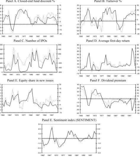
Prior work suggests a number of proxies for sentiment to use as time-series conditioning variables. There are no definitive or uncontroversial measures, however. We therefore form a composite index of sentiment that is based on the common variation in six underlying proxies for sentiment: the closed-end fund discount, NYSE share turnover, the number and average first-day returns on IPOs, the equity share in new issues, and the dividend premium. The sentiment proxies are measured annually from 1962 to 2001. We first introduce each proxy separately, and then discuss how they are formed into overall sentiment indexes.
The closed-end fund discount,CEFD, is the average difference between the
net asset values (NAV) of closed-end stock fund shares and their market prices.
Prior work suggests thatCEFDis inversely related to sentiment. Zweig (1973)
1656 The Journal of Finance
through 1993 from Neal and Wheatley (1998), for 1994 through 1998 from CDA/Wiesenberger, and for 1999 through 2001 from turn-of-the-year issues of theWall Street Journal.
NYSE share turnover is based on the ratio of reported share volume to
av-erage shares listed from theNYSE Fact Book. Baker and Stein (2004) suggest
that turnover, or more generally liquidity, can serve as a sentiment index: In a market with short-sales constraints, irrational investors participate, and thus add liquidity, only when they are optimistic; hence, high liquidity is a symp-tom of overvaluation. Supporting this, Jones (2001) finds that high turnover forecasts low market returns. Turnover displays an exponential, positive trend over our period and the May 1975 elimination of fixed commissions also has a
visible effect. As a partial solution, we defineTURN as the natural log of the
raw turnover ratio, detrended by the 5-year moving average.
The IPO market is often viewed as sensitive to sentiment, with high first-day returns on IPOs cited as a measure of investor enthusiasm, and the low idiosyncratic returns on IPOs often interpreted as a symptom of market timing
(Stigler (1964), Ritter (1991)). We take the number of IPOs, NIPO, and the
average first-day returns,RIPO, from Jay Ritter’s website, which updates the
sample in Ibbotson, Sindelar, and Ritter (1994).
The share of equity issues in total equity and debt issues is another measure of financing activity that may capture sentiment. Baker and Wurgler (2000) find that high values of the equity share predict low market returns. The equity share is defined as gross equity issuance divided by gross equity plus gross
long-term debt issuance using data from theFederal Reserve Bulletin.8
Our sixth and last sentiment proxy is the dividend premium,PD−ND, the log
difference of the average market-to-book ratios of payers and nonpayers. Baker and Wurgler (2004) use this variable to proxy for relative investor demand for dividend-paying stocks. Given that payers are generally larger, more profitable firms with weaker growth opportunities (Fama and French (2001)), the divi-dend premium may proxy for the relative demand for this correlated bundle of characteristics.
Each sentiment proxy is likely to include a sentiment component as well as idiosyncratic, non-sentiment-related components. We use principal components analysis to isolate the common component. Another issue in forming an index is determining the relative timing of the variables—that is, if they exhibit lead-lag relationships, some variables may reflect a given shift in sentiment earlier than others. For instance, Ibbotson and Jaffe (1975), Lowry and Schwert (2002), and Benveniste et al. (2003) find that IPO volume lags the first-day returns on IPOs. Perhaps sentiment is partly behind the high first-day returns, and this attracts additional IPO volume with a lag. More generally, proxies that involve
firm supply responses (S and NIPO) can be expected to lag behind proxies
8While they both reflect equity issues, the number of IPOs and the equity share have important
that are based directly on investor demand or investor behavior (RIPO, PD−ND,
TURN, andCEFD).
We form a composite index that captures the common component in the six proxies and incorporates the fact that some variables take longer to reveal the
same sentiment.9We start by estimating the first principal component of the
six proxies and their lags. This gives us a first-stage index with 12 loadings, one for each of the current and lagged proxies. We then compute the correla-tion between the first-stage index and the current and lagged values of each
of the proxies. Finally, we define SENTIMENTas the first principal
compo-nent of the correlation matrix of six variables—each respective proxy’s lead or lag, whichever has higher correlation with the first-stage index—rescaling the coefficients so that the index has unit variance.
This procedure leads to a parsimonious index
SENTIMENTt = −0.241CEFDt+0.242TURNt−1+0.253NIPOt
+0.257RIPOt−1+0.112St−0.283PtD−−1ND, (2) where each of the index components has first been standardized. The first principal component explains 49% of the sample variance, so we conclude that one factor captures much of the common variation. The correlation between the
12-term first-stage index and theSENTIMENTindex is 0.95, suggesting that
little information is lost in dropping the six terms with other time subscripts. TheSENTIMENTindex has several appealing properties. First, each indi-vidual proxy enters with the expected sign. Second, all but one enters with
the expected timing; with the exception ofCEFD, price and investor behavior
variables lead firm supply variables. Third, the index irons out some extreme observations. (The dividend premium and the first-day IPO returns reached unprecedented levels in 1999, so for these proxies to work as individual predic-tors in the full sample, these levels must be matched exactly to extreme future returns.)
One might object to equation (2) as a measure of sentiment on the grounds that the principal components analysis cannot distinguish between a common sentiment component and a common business cycle component. For instance, the number of IPOs varies with the business cycle in part for entirely rational
reasons. We want to identify when the number of IPOs is high fornogood reason.
We therefore construct a second index that explicitly removes business cycle variation from each of the proxies prior to the principal components analysis.
Specifically, we regress each of the six raw proxies on growth in the indus-trial production index (Federal Reserve Statistical Release G.17), growth in consumer durables, nondurables, and services (all from BEA National Income Accounts Table 2.10), and a dummy variable for NBER recessions. The
residu-als from these regressions, labeled with a superscript⊥, may be cleaner proxies
for investor sentiment. We form an index of the orthogonalized proxies following the same procedure as before. The resulting index is
9See Brown and Cliff (2004) for a similar approach to extracting a sentiment factor from a set
1658 The Journal of Finance
SENTIMENTt⊥ = −0.198CEFD⊥t +0.225TURNt⊥−1+0.234NIPO
⊥
t
+0.263RIPOt⊥−1+0.211S
⊥
t −0.243P D−ND,⊥
t−1 . (3) Here, the first principal component explains 53% of the sample variance of the orthogonalized variables. Moreover, only the first eigenvalue is above 1.00. In
terms of the signs and the timing of the components, SENTIMENT⊥ retains
all of the appealing properties ofSENTIMENT.
Table II summarizes and correlates the sentiment measures, and Figure 1 plots them. The figure shows immediately that orthogonalizing to macro vari-ables is a second-order issue. It does not qualitatively affect any component of the index or the overall index (see Panel E). Indeed, Table II suggests that
on balance the orthogonalized proxies are slightlymore correlated with each
other than are the raw proxies. If the raw variables were driven by common macroeconomic conditions (that we failed to remove through orthogonalization) instead of common investor sentiment, one would expect the opposite. In any case, to demonstrate robustness we present results for both indexes in our main analysis.
More importantly, Figure 1 shows that the sentiment measures roughly line up with anecdotal accounts of fluctuations in sentiment. Most proxies point to low sentiment in the first few years of the sample, after the 1961 crash in growth stocks. Specifically, the closed-end fund discount and dividend premium are high, while turnover and equity issuance-related variables are low. Each variable identifies a spike in sentiment in 1968 and 1969, again matching anec-dotal accounts. Sentiment then tails off until, by the mid 1970s, it is low by most measures (recall that for turnover this is confounded by deregulation). The late 1970s through mid 1980s sees generally rising sentiment, and, according to the composite index, sentiment has not dropped far below a medium level since 1980. At the end of 1999, near the peak of the Internet bubble, sentiment is high
by most proxies. Overall,SENTIMENT⊥ is positive for the years 1968–1970,
1972, 1979–1987, 1994, 1996–1997, and 1999–2001. This correspondence with anecdotal accounts seems to confirm that the measures capture the intended variation.
Investor
Sentiment
and
the
Cross-Section
of
Stoc
k
Returns
1659
Means, standard deviations, and correlations for measures of investor sentiment. In the first panel, we present raw sentiment proxies. The first (CEFD) is the year-end, value-weighted average discount on closed-end mutual funds. The data on prices and net asset values (NAVs) come from Neal and Wheatley (1998) for 1962 through 1993, CDA/Wiesenberger for 1994 through 1998, and turn-of-the-year issues of theWall Street Journalfor 1999 and 2000. The second measure (TURN) is detrended natural log turnover. Turnover is the ratio of reported share volume to average shares listed from the NYSE Fact Book. We detrend using the past 5-year average. The third measure (NIPO) is the annual number of initial public offerings. The fourth measure (RIPO) is the average annual first-day returns of initial public offerings. Both IPO series come from Jay Ritter, updating data analyzed in Ibbotson, Sindelar, and Ritter (1994). The fifth measure (S) is gross annual equity issuance divided by gross annual equity plus debt issuance from Baker and Wurgler (2000). The sixth measure (PD−ND) is the year-end log ratio of the value-weighted average market-to-book ratios of payers and nonpayers from Baker and Wurgler
(2004). Turnover, the average annual first-day return, and the dividend premium are lagged 1 year relative to the other three measures.SENTIMENTis the first principal component of the six sentiment proxies. In the second panel, we regress each of the six proxies on the growth in industrial production, the growth in durable, nondurable, and services consumption, the growth in employment, and a flag for NBER recessions. The orthogonalized proxies, labeled with a “⊥,” are the residuals from these regressions.SENTIMENT⊥is the first principal component of the six orthogonalized proxies. Superscripts
a, b, and c denote statistical significance at the 1%, 5%, and 10% level, respectively.
Correlations with Sentiment Correlations with Sentiment Components
Mean SD Min Max SENTIMENT SENTIMENT⊥ CEFD TURN NIPO RIPO S PD−ND
Panel A: Raw Data
CEFDt 9.03 8.12 −10.41 23.70 −0.71a −0.60a 1.00
TURNt−1 11.99 18.27 −26.70 42.96 0.71a 0.68a −0.29c 1.00
NIPOt 358.41 262.76 9.00 953.00 0.74a 0.66a −0.55a 0.38b 1.00
RIPOt−1 16.94 14.93 −1.67 69.53 0.76a 0.80a −0.42a 0.50a 0.35b 1.00
St 19.53 8.34 7.83 43.00 0.33b 0.44a −0.01 0.30c 0.16 0.26 1.00
PD−ND
t−1 0.20 18.67 −33.17 36.06 −0.83a −0.76a 0.52a −0.50a −0.56a −0.58a −0.12 1.00
Panel B: Controlling for Macroeconomic Conditions
CEFD⊥
t 0.00 6.25 −18.32 9.60 −0.62a −0.63a 1.00
TURN⊥
t−1 0.00 15.49 −26.03 26.37 0.69a 0.71a −0.26 1.00 NIPO⊥
t 0.00 226.30 −435.98 484.15 0.73a 0.74a −0.45a 0.39b 1.00
RIPO⊥
t−1 0.00 14.31 −23.55 46.54 0.77a 0.83a −0.46a 0.53a 0.44a 1.00 S⊥
t 0.00 6.15 −12.17 14.29 0.55a 0.67a −0.41a 0.32b 0.50a 0.47a 1.00
PD−ND⊥
1660 The Journal of Finance
Panel A. Closed-end fund discount %
-15 -10 -5 0 5 10 15 20 25 30
1962 1967 1972 1977 1982 1987 1992 1997 -20 -15 -10 -5 0 5 10 15
Panel B. Turnover %
-40 -30 -20 -10 0 10 20 30 40 50
1962 1967 1972 1977 1982 1987 1992 1997 -30 -20 -10 0 10 20 30
Panel C. Number of IPOs
0 200 400 600 800 1000 1200
1962 1967 1972 1977 1982 1987 1992 1997 -600 -400 -200 0 200 400 600
Panel D. Average first-day return
-10 0 10 20 30 40 50 60 70 80
1962 1967 1972 1977 1982 1987 1992 1997 -30 -20 -10 0 10 20 30 40 50 60
Panel E. Equity share in new issues
0 5 10 15 20 25 30 35 40 45 50
1962 1967 1972 1977 1982 1987 1992 1997 -15 -10 -5 0 5 10 15 20
Panel F. Dividend premium
-40 -30 -20 -10 0 10 20 30 40
1962 1967 1972 1977 1982 1987 1992 1997 -50 -40 -30 -20 -10 0 10 20 30 40 50
Panel E. Sentiment index (SENTIMENT)
-3.0 -2.0 -1.0 0.0 1.0 2.0 3.0
1962 1967 1972 1977 1982 1987 1992 1997 -3.0 -2.0 -1.0 0.0 1.0 2.0 3.0
IV. Empirical Tests
A. Sorts
Table III looks for conditional characteristics effects in a simple, nonpara-metric way. We place each monthly return observation into a bin according to the decile rank that a characteristic takes at the beginning of that month, and
then according to the level ofSENTIMENT⊥at the end of the previous
calen-dar year. To keep the meaning of the deciles similar over time, we define them based on NYSE firms. The trade-off is that there is not a uniform distribution of firms across bins in any given month. We compute the equal-weighted average monthly return for each bin and look for patterns. In particular, we identify
time-series changes in cross-sectional effects from the conditionaldifferenceof
average returns across deciles.
The first rows of Table III show the effect of size, as measured byME,
con-ditional on sentiment. These rows reveal that the size effect of Banz (1981) appears in low sentiment periods only. Specifically, Table III shows that when
SENTIMENT⊥ is negative, returns average 2.37% per month for the bottom
MEdecile and 0.92 for the top decile. A similar pattern is apparent when
con-ditioning onCEFD(not reported). A link between the size effect and closed-end
fund discounts is also noted by Swaminathan (1996). This pattern is consistent with some long-known results. Namely, the size effect is essentially a January effect (Keim (1983), Blume and Stambaugh (1983)), and the January effect, in turn, is stronger after a period of low returns (Reinganum (1983)), which is also when sentiment is likely to be low.
As an aside, note that the average returns across the first two rows of Table III illustrate that subsequent returns tend to be higher, across most of the cross-section, when sentiment is low. This is consistent with prior results that the equity share and turnover, for example, forecast market returns. More gen-erally, it supports our premise that sentiment has broad effects, and so the existence of richer patterns within the cross-section is not surprising.
The conditional cross-sectional effect of Age is striking. In general,
in-vestors appear to demand young stocks when SENTIMENT⊥ is positive and
prefer older stocks when sentiment is negative. For example, when
senti-ment is pessimistic, top-decile Age firms return 0.54% per month less than
bottom-decile Age firms. However, they return 0.85% more when sentiment
is optimistic. When sentiment is positive, the effect is concentrated in the very youngest stocks, which are recent IPOs; when it is negative, the con-trast is between the bottom and top several deciles of age. Overall, there is a nearly monotonic effect in the conditional difference of returns. This
re-sult is intriguing because Age has no unconditional effect.10 The strong
con-ditional effects, of opposite sign, average out across high and low sentiment periods.
10This conclusion is in seeming contrast to Barry and Brown’s (1984) evidence of an
1662
T
he
J
ournal
of
F
inance
Table III
Future Returns by Sentiment Index and Firm Characteristics, 1963–2001
For each month, we form 10 equal-weighted portfolios according to the NYSE breakpoints of firm size (ME),age, total risk, earnings-book ratio for profitable firms (E/BE), dividend-book ratio for dividend payers (D/BE), fixed assets (PPE/A), research and development (RD/A), book-to-market ratio (BE/ME), external finance over assets (EF/A), and sales growth (GS). We also calculate portfolio returns for unprofitable firms, nonpayers, zero-PP&E firms, and zero-R&D firms. We then report average portfolio returns over months in whichSENTIMENT⊥
from the previous year-end is positive, months in which it is negative, and the difference between these two averages.SENTIMENT⊥is positive for 1968–1970, 1972, 1979–1987, 1994,
1996–1997, and 1999–2001 (the return series ends in 2001, so the last value used is 2000).
Decile Comparisons
SENTIMENT⊥
t−1 ≤0 1 2 3 4 5 6 7 8 9 10 10−1 10−5 5−1 >0–≤0
ME Positive 0.73 0.74 0.85 0.83 0.92 0.84 1.06 0.99 1.02 0.98 0.26 0.06 0.20
Negative 2.37 1.68 1.66 1.51 1.67 1.35 1.26 1.25 1.05 0.92 −1.45 −0.75 −0.70
Difference −1.65 −0.93 −0.81 −0.68 −0.75 −0.51 −0.20 −0.26 −0.03 0.06 1.71 0.81 0.90
Age Positive 0.25 0.83 0.94 0.95 1.18 1.19 0.96 1.18 1.09 1.11 0.85 −0.07 0.93
Negative 1.77 1.88 1.97 1.68 1.70 1.68 1.38 1.34 1.36 1.24 −0.54 −0.46 −0.08
Difference −1.52 −1.05 −1.03 −0.74 −0.51 −0.49 −0.42 −0.16 −0.27 −0.13 1.39 0.39 1.00
σ Positive 1.44 1.41 1.25 1.20 1.24 1.08 1.01 0.88 0.75 0.30 −1.14 −0.94 −0.20
Negative 1.01 1.17 1.26 1.37 1.52 1.61 1.65 1.83 2.08 2.41 1.40 0.89 0.51
Difference 0.43 0.24 −0.01 −0.16 −0.28 −0.53 −0.65 −0.95 −1.33 −2.11 −2.54 −1.84 −0.71
E/BE Positive 0.35 0.68 0.85 0.86 0.89 0.92 0.88 0.92 1.05 1.10 0.93 0.24 0.01 0.24 0.61
Negative 2.59 2.24 2.10 2.26 1.82 1.65 1.79 1.62 1.59 1.43 1.57 −0.67 −0.08 −0.59 −0.95
Difference −2.25 −1.56 −1.25 −1.40 −0.93 −0.73 −0.91 −0.70 −0.54 −0.34 −0.65 0.91 0.09 0.82 1.56
D/BE Positive 0.44 1.08 1.09 1.29 1.11 1.24 1.17 1.31 1.24 1.19 1.15 0.07 −0.09 0.16 0.75
Negative 2.32 1.87 1.63 1.59 1.51 1.38 1.30 1.20 1.12 1.16 1.18 −0.69 −0.19 −0.49 −0.89
Difference −1.88 −0.79 −0.54 −0.30 −0.40 −0.14 −0.14 0.11 0.12 0.03 −0.03 0.76 0.11 0.65 1.64
PPE/A Positive 1.31 0.48 0.66 0.74 0.81 1.04 0.90 0.79 0.87 1.04 1.05 0.57 0.02 0.56 −0.53
Negative 1.26 1.93 1.96 1.90 1.87 1.82 1.89 1.66 1.56 1.29 1.62 −0.31 −0.20 −0.11 0.53
Difference 0.05 −1.45 −1.31 −1.17 −1.07 −0.78 −0.99 −0.87 −0.69 −0.25 −0.56 0.88 0.22 0.67 −1.05
RD/A Positive 0.80 1.21 1.04 1.37 1.37 1.34 1.22 1.24 1.29 1.39 1.38 0.17 0.04 0.13 0.55
Negative 1.63 1.57 1.47 1.58 1.73 1.66 1.81 1.97 2.04 2.13 2.44 0.87 0.78 0.09 0.43
Difference −0.83 −0.36 −0.43 −0.22 −0.36 −0.32 −0.60 −0.73 −0.75 −0.74 −1.05 −0.69 −0.74 0.04 0.12
BE/ME Positive 0.03 0.61 0.82 0.87 0.96 1.09 1.17 1.18 1.29 1.27 1.24 0.31 0.93
Negative 1.41 1.43 1.46 1.54 1.61 1.69 1.87 1.94 2.18 2.45 1.04 0.84 0.20
Difference −1.38 −0.81 −0.64 −0.67 −0.65 −0.60 −0.70 −0.76 −0.88 −1.18 0.20 −0.53 0.73
EF/A Positive 1.08 1.04 1.25 1.18 1.19 1.17 1.02 0.92 0.75 −0.01 −1.09 −1.20 0.11
Negative 2.43 2.09 1.85 1.75 1.59 1.53 1.51 1.51 1.71 1.53 −0.90 −0.06 −0.84
Difference −1.35 −1.05 −0.59 −0.57 −0.40 −0.35 −0.49 −0.60 −0.96 −1.54 −0.18 −1.14 0.96
GS Positive 0.70 1.07 1.19 1.15 1.21 1.18 1.22 1.10 0.81 0.05 −0.65 −1.16 0.51
Negative 2.49 1.78 1.61 1.54 1.47 1.57 1.68 1.78 1.68 1.69 −0.80 0.22 −1.02
Panel A. ME -2.5 -2.0 -1.5 -1.0 -0.5 0.0 0.5 1.0 1.5 2.0 2.5 3.0
1 2 3 4 5 6 7 8 9 10
1
Panel B. Age
-2.5 -2.0 -1.5 -1.0 -0.5 0.0 0.5 1.0 1.5 2.0 2.5 3.0
1 2 3 4 5 6 7 8 9 10
Panel C. Total Risk
-2.5 -2.0 -1.5 -1.0 -0.5 0.0 0.5 1.0 1.5 2.0 2.5 3.0
1 2 3 4 5 6 7 8 9 10
Panel D. Earnings
-2.5 -2.0 -1.5 -1.0 -0.5 0.0 0.5 1.0 1.5 2.0 2.5 3.0
0 1 2 3 4 5 6 7 8 9 10
Panel E. Dividends
-2.5 -2.0 -1.5 -1.0 -0.5 0.0 0.5 1.0 1.5 2.0 2.5 3.0
0 1 2 3 4 5 6 7 8 9 10
Panel F. PPE/A
-2.5 -2.0 -1.5 -1.0 -0.5 0.0 0.5 1.0 1.5 2.0 2.5 3.0
0 1 2 3 4 5 6 7 8 9 10 Panel G. RD/A
-2.5 -2.0 -1.5 -1.0 -0.5 0.0 0.5 1.0 1.5 2.0 2.5 3.0
0 1 2 3 4 5 6 7 8 9 10
Panel H. BE/ME
-2.5 -2.0 -1.5 -1.0 -0.5 0.0 0.5 1.0 1.5 2.0 2.5 3.0
1 2 3 4 5 6 7 8 9 10
Panel I. EF/A
-2.5 -2.0 -1.5 -1.0 -0.5 0.0 0.5 1.0 1.5 2.0 2.5 3.0
1 2 3 4 5 6 7 8 9 10
Panel J. GS
-2.5 -2.0 -1.5 -1.0 -0.5 0.0 0.5 1.0 1.5 2.0 2.5 3.0
1 2 3 4 5 6 7 8 9 10
Figure 2. Two-way sorts: Future returns by sentiment index and firm characteristics, 1963–2001.For each month, we form 10 portfolios according to the NYSE breakpoints of firm size (ME), age, total risk, earnings-book ratio for profitable firms (E/BE), dividend-book ratio for payers (D/BE), fixed assets (PPE/A), research and development (RD/A), book-to-market ratio (BE/ME), external finance over assets (EF/A), and sales growth (GS). We also calculate portfolio returns for unprofitable, nonpaying, zero-PP&E, and zero-R&D firms. The solid bars are returns following pos-itiveSENTIMENT⊥periods, and the clear bars are returns following negative sentiment periods. The dashed line is the average across both periods and the solid line is the difference. SENTI-MENT⊥ is positive for 1968–1970, 1972, 1979–1987, 1994, 1996–1997, and 1999–2001 (returns end in 2001, so the last value used is 2000).
The next rows of Table III indicate that the cross-sectional effect of return volatility is conditional on sentiment in the hypothesized manner. In particular, highSigmastocks appear to be out of favor when sentiment is low, as they earn
returns of 2.41% per month over the next year. However, just as with Age,
the cross-sectional effect ofSigmafully reverses in low sentiment conditions.
Loosely speaking, when sentiment is high, “riskier” stocks earnlowerreturns.
When sentiment is low, they earnhigherreturns. A natural interpretation is
that highly volatile stocks are, like young stocks, relatively hard to value and relatively hard to arbitrage, making them especially prone to fluctuations in sentiment.
Figure 2 shows the results of Table III graphically. Panel C, for example,
shows the unconditional average monthly returns acrossSigmadeciles (dashed
1664 The Journal of Finance
deciles; and the difference in conditional returns (solid line). The solid line
summarizes the difference in the relationship betweenSigmaand future
re-turns across the two regimes and clearly illustrates that the future rere-turns on highSigmastocks are more sensitive to sentiment.
The next rows examine profitability and dividends. For average investors, perhaps the most salient comparisons are simply those between profitable and
unprofitable (E<0) firms and payers and nonpayers (D=0). These contrasts
are in the extreme right column, where we average returns across profitable (paying) firms and compare them to unprofitable (nonpaying) firms. These characteristics again display intriguing conditional sign-flip patterns. When sentiment is positive, monthly returns over the next year are 0.61% higher on profitable than unprofitable firms and 0.75% higher on payers than nonpayers.
When it is negative, however, returns are 0.95% per monthloweron profitable
firms and 0.89% lower on payers. The left column shows that these patterns are driven mostly by conditional variation in the returns of unprofitable and nonpaying firms, although there are also some differences across levels of div-idend payments and profitability. Again, this is consistent with unprofitable, nonpaying firms being generally harder both to value and to arbitrage, thus exposing them more to sentiment fluctuations.
The next two rows look at asset tangibility characteristics under the notion that firms with less tangible assets may be more difficult to value. The patterns here are not so strong, but there is a suggestion that firms with more intangible
assets, as measured by lessPPE/A, are more sensitive to fluctuations in
senti-ment. (This pattern is only apparent within firms that report positivePPE/A.)
The clearest pattern inRD/Ais a modest unconditional effect in which higher
RD/Afirms earn higher returns.
The remaining variables—book-to-market, external finance, and sales growth—also display intriguing patterns. Most simply, running across rows, one can see that each of them has some unconditional explanatory power.
Fu-ture returns are generally higher for highBE/MEstocks, lowEF/Astocks, and
lowGSdecile stocks. TheEF/Aresult is reminiscent of Loughran and Ritter
(1995) and Spiess and Affleck-Graves (1995, 1999), while theGSresult is
sug-gested in Lakonishok, Shleifer, and Vishny (1994).
A closer look reveals that after controlling for these unconditional effects, a conditional pattern emerges. Specifically, there is a U-shaped pattern in the
conditional difference. Consider theGSvariable. The difference in returns on
bottom-decileGSfirms is−1.79% per month. For fifth-decile firms, the
differ-ence is only −0.26% per month. But for tenth-decile firms, the difference is
again large,−1.64% per month. U-shaped patterns also appear in the
condi-tional difference row forBE/MEand EF/A. The solid lines in Panels H–J of
Figure 2 show these “frowns” graphically. The figure illustrates why one must control for the strong unconditional effects in these variables in order to see the conditional effects.
the U reflect? It reflects the multidimensional nature of the growth and
dis-tress variables. ConsiderGS. High-GSfirms include high-flying growth firms,
low-GSfirms are often distressed firms with shrinking sales, and middle-GS
firms are steady, slow-growth firms. Thus, relative to firms in the middle deciles,
firms with extreme values ofGSare harder to value, and perhaps to arbitrage,
and thus may be more sensitive to sentiment. Put differently, firms with
ex-treme values of GSare likely to seem riskier, in a salient sense, than firms
in the middle. The same explanation may help to explain the U-shaped
pat-terns in the conditional difference row ofEF/AandBE/ME. There again, low
EF/Afirms and highBE/MEfirms include distressed firms, highEF/Aand low
BE/MEfirms include high-flyers, and the middle deciles tend to be populated
by the most “stable” firms.
In unreported results, we sort returns not just on positive and negative values ofSENTIMENT⊥but also on>1 and<−1 standard deviation values. Not
sur-prisingly, conditioning on more extreme values of sentiment leads to stronger results. We take more formal account of the continuous nature of the sentiment
indexes in the next subsection. Also, for brevity, we omit sorts onSENTIMENT
(the nonorthogonalized version), which give similar results. We present results for both indexes in the next section. Finally, we have also sorted returns on
positive and negativeSENTIMENT⊥, where positive and negative are defined
relative to a 10-year average. By requiring a 10-year history of sentiment, one loses a little more than one-quarter of the sample. The results are qualitatively
identical to those in Table III, although slightly weaker except forAge, which
is slightly stronger.
B. Predictive Regressions for Long–Short Portfolios
Another way to look for conditional characteristics effects is to use sentiment to forecast equal-weighted portfolios that are long on stocks with high values of a characteristic and short on stocks with low values. Above we see that the aver-age payer, for example, earns higher returns than the averaver-age nonpayer when sentiment is high, so sentiment seems likely to forecast a long–short portfolio formed on dividend payment. But a regression approach allows us to conduct formal significance tests, incorporate the continuous nature of the sentiment indexes, and determine which characteristics have conditional effects that are distinct from well-known unconditional effects.
Table IV starts by plotting the average monthly returns on various long–short portfolios over time. The first several rows show that, not surprisingly, long–
short portfolios formed on size (SMB), age, volatility, profitability, dividend
payment, and (to a lesser extent) tangibility are typically highly correlated. Thus, a good question, which we address in subsequent tables, is whether the results from the sorts are all part of the same pattern or are somewhat distinct. This question is also relevant given that our portfolios are equal-weighted. By
controlling for SMBin portfolio forecasting regressions, we can examine the
1666
T
he
J
ournal
of
F
inance
Table IV
Correlations of Portfolio Returns, 1963–2001
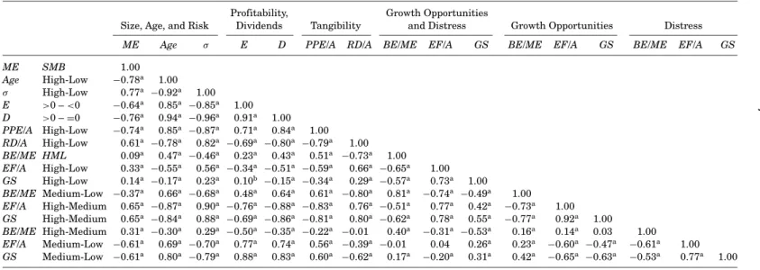
Correlations among characteristics-based portfolios. The sample period includes monthly returns from 1963 to 2001. The long–short portfolios are formed based on firm characteristics: firm size (ME),age, total risk (σ), profitability (E), dividends (D), fixed assets (PPE), research and development (RD), book-to-market ratio (BE/ME), external finance over assets (EF/A), and sales growth decile (GS). High is defined as a firm in the top three NYSE deciles, low is defined as a firm in the bottom three NYSE deciles, and medium is defined as a firm in the middle four NYSE deciles. Superscripts a, b, and c denote statistical significance at the 1%, 5%, and 10%, level, respectively.
Profitability, Growth Opportunities
Size, Age, and Risk Dividends Tangibility and Distress Growth Opportunities Distress
ME Age σ E D PPE/A RD/A BE/ME EF/A GS BE/ME EF/A GS BE/ME EF/A GS
ME SMB 1.00
Age High-Low −0.78a 1.00
In the last several rows of Table IV, we break the growth and distress vari-ables into “high minus medium” and “medium minus low” portfolios. In the case
of theGSvariable, for example, these portfolios are highlynegativelycorrelated
with each other, at−0.63, indicating that high and lowGSfirms actually move
together relative to middleGSfirms. Likewise, the correlation between “high
minus medium” and “medium minus low”EF/Ais−0.60. Thus, simple “high
minus low” analyses of these variables would omit crucial aspects of the cross-section.
The question is whether sentiment can predict the various long–short
port-folios analyzed in Table IV. We run regressions of the type11
RXit=High,t−RXit=Low,t=c+dSENTIMENTt−1+uit. (4) The dependent variable is the monthly return on a long–short portfolio, such
as SMB, and the monthly returns from January through December of t are
regressed on the sentiment index that prevailed at the end of the prior year. We also distinguish novel predictability effects from well-known comovement using the multivariate regression
RXit=High,t−RXit=Low,t=c+d SENTIMENTt−1+βRMKTt+sSMBt
+hHMLt+mUMDt+uit. (5)
The variable RMRF is the excess return of the value-weighted market over
the risk-free rate. The variableUMDis the return on high-momentum stocks
minus the return on low-momentum stocks, where momentum is measured
over months [−12,−2]. As described in Fama and French (1993),SMBis the
return on portfolios of small and bigMEstocks that is separate from returns on
HML, whereHMLis constructed to isolate the difference between high and low
BE/MEportfolios.12We excludeSMBandHMLfrom the right side when they
are the portfolios being forecast. Standard errors are bootstrapped to correct for the bias induced if the autocorrelated sentiment index has innovations that are correlated with innovations in portfolio returns, as in Stambaugh (1999).
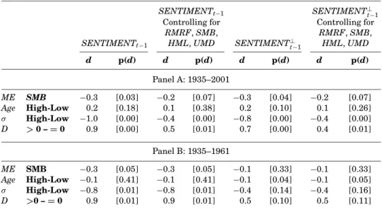
Table V shows the results. The results provide formal support to our pre-liminary impressions from the sorts. In particular, the first panel shows that when sentiment is high, returns on small, young, and high volatility firms are relatively low over the coming year. The coefficient on sentiment diminishes
once we control forRMRF, SMB,HML, andUMD, but in most cases the
signif-icance of the predictive effect does not depend on including or excluding these
controls. In terms of magnitudes, the coefficient for predictingSMB, for
exam-ple, indicates that a one-unit increase in sentiment (which equals a one-SD
increase, because the indexes are standardized) is associated with a −0.40%
lower monthly return on the small minus large portfolio.
11Intuitively, in terms of equation (1), this amounts to a regression of (b
1X+b2Tt−1X) on
1668 The Journal of Finance
Table V also shows that the coefficients onSENTIMENTandSENTIMENT⊥
are very similar. Keep in mind that the coefficients onSENTIMENT⊥are
essen-tially the same as one would find from regressing long–short portfolio returns directly on a raw sentiment index and controls for contemporaneous
macroeco-nomic conditions—that is, regressingXonZand using the residuals to predict
Y is equivalent to regressingY onX and Z. The similarity of the results on
SENTIMENT and SENTIMENT⊥ thus suggests that macroeconomic
condi-tions play a minor role.
For profitability and dividend payment, we run regressions to predict the difference between the profitable and paying portfolios and the unprofitable and nonpaying portfolios, respectively, because the sorts suggest that these are likely to capture the main contrasts. The results show that sentiment indeed has significant predictive power for these portfolios, with higher sentiment fore-casting relatively higher returns on payers and profitable firms. The patterns
are little affected by controlling forRMRF,SMB,HML, andUMD.
As we find with the sorts, the tangibility characteristics do not exhibit strong conditional effects. Sentiment does have marginal predictive power for the
PPE/Aportfolio, with high sentiment associated with relatively low future
re-turns on low PPE/Astocks, but this disappears after controlling for RMRF,
SMB,HML, andUMD. The coefficients on theRD/Aportfolio forecasts are not
consistent in sign or magnitude.
Also as we find with the sorts, the “growth and distress” variables do not have simple monotonic relationships with sentiment. Panel D shows that sentiment
does not predict simple high minus low portfolios formed on any of BE/ME,
EF/A, orGS. However, Panels E and F show that when the multidimensional
nature of these variables is incorporated, there is much stronger evidence of predictive power. We separate extreme growth opportunities effects from dis-tress effects by constructing High, Medium, and Low portfolios based on the top three, middle four, and bottom three NYSE decile breakpoints, respectively. The results show that when sentiment is high, subsequent returns on both
lowandhigh sales growth firms are low relative to returns on medium growth
firms. This illustrates the U-shaped pattern in Table III in a different way, and shows that it is statistically significant. An equally significant U-shaped pattern is apparent with external finance; when sentiment is high, subsequent
returns on both lowandhigh external finance firms are low relative to more
typical firms. In the case ofBE/ME, however, although sentiment predicts the
high minus medium and medium minus low portfolios with opposite signs, neither coefficient is reliably significant. This matches our inferences from the sorts, where we see that the U-shaped pattern in the conditional difference for
BE/MEis somewhat weaker than forEF/AandGS.