A Simple FEM Formulation Applied to Nonlinear Problems of Impact with Thermomechanical Coupling

Abstract

The thermal effects of problems involving deformable structures are essential to describe the behavior of materials in feasible terms. Verifying the transformation of mechanical energy into heat it is possible to predict the modifications of mechanical properties of materials due to its temperature changes. The current paper presents the numerical development of a finite element method suitable for nonlinear structures coupled with thermomechanical behavior; including impact problems. A simple and effective alternative formulation is presented, called FEM positional, to deal with the dynamic nonlinear systems. The developed numerical is based on the minimum potential energy written in terms of nodal positions instead of displacements. The effects of geometrical, material and thermal nonlinearities are considered. The thermodynamically consistent formulation is based on the laws of thermodynamics and the Helmholtz free-energy, used to describe the thermoelastic and the thermoplastic behaviors. The coupled thermomechanical model can result in secondary effects that cause redistributions of internal efforts, depending on the history of deformation and material properties. The numerical results of the proposed formulation are compared with examples found in the literature.

Keywords

Positional Formulation; Nonlinear analysis; Thermomechanical; Coupled problems; Impact.

A Simple FEM Formulation Applied to Nonlinear

Problems of Impact with Thermomechanical Coupling

1 INTRODUCTION

The current paper presents the study of thermomechanical response for frictionless impact problems, considering the nonlinear behavior through a simple formulation based on FEM, called positional.

João Paulo de Barros Cavalcante a Daniel Nelson Maciel b, *

Marcelo Greco c

José Neres da Silva Filho a

a _{Civil Engineering Department, Federal}

University of Rio Grande do Norte, Lagoa Nova, 59078-900, Natal, RN, Brazil.

b _{School of Sciences and Technology,}

Federal University of Rio Grande do Norte, Lagoa Nova, 59078-900, Natal, RN, Brazil.

c _{Structural Engineering Department,}

Federal University of Minas Gerais, Avenida Presidente Carlos, 31270-901, Belo Horizonte, MG, Brazil.

* Corresponding author. E-mail address: dnmaciel@ect.ufrn.br

http://dx.doi.org/10.1590/1679-78253737

The formulation is described in Total Lagrangian reference using as unknowns the nodal positions instead of the displacement. This formulation shows a simple language in respect to nonlinear geometric approach where the main advantage is the absence of co-rotational axes (the formulation can be carried on directly with global axes only) (Coda and Greco, 2004; Greco and Coda, 2006; Carrazedo and Coda, 2010; Coda and Paccola, 2011; Coda et al., 2013).

Duhamel in 1837 and Neumann in 1885 identified the modification need of the mechanical models to consider the temperature differences to accurately represent the behavior of the materials (Sherief et al., 2004). The thermomechanical theory investigates the interaction between temperature and structural strains. In many cases, the influence of the strains in relation to the thermal field may be neglected. This results in thermomechanical uncoupled system, for which only the effect of temperature modifies the strains field. The experimental studies and theoretical models of thermomechanical have advanced simultaneously. The use of more sophisticated experiments results in more accurate and efficient mathematical models.

The thermoelasticity and thermoplasticity are defined as part of the thermomechanical theory that determines the behavior of elastic and plastic bodies, respectively, submitted to thermal and mechanical efforts. The first studies were devoted to static problems. Danilovskaya (1950) was the first researcher that tried to include the effects of inertia in thermoelastic transient problems. These problems presented simple nature, but the solution explained the process of transmission of the thermal stresses. The theory of uncoupled thermoelasticity may not be satisfactory for some transient problems, because experimental observations that shown the thermal field modified by the strains field. Several experiments emphasize the influence of strains on thermal field (Rittel, 1998; Benzerga et al., 2005; Stanley, 2008).

Biot (1956) developed the classical theory of coupled thermoelasticity. The equations of elasticity and heat conduction are interdependent. The equations used to describe this theory are a combination between the elasticity theory and the laws of thermodynamics. The equations that represent the heat conduction are parabolic and heat propagation velocity in an elastic system is infinite. The theory of generalized thermoelasticity came to deal with these inconsistencies observed in experimental results. The general theory of thermoelasticity has been modified over the years. The first theory proposed by Lord and Shulman (1967) considers that the heat conduction law is altered to consider the heat flux and its rate. It was considered a time parameter relaxation to ensure finite velocity of propagation of heat. The second theory developed by Green and Lindsay (1972) considers that the constitutive equations are modified by insertion of two time parameters relaxation. Green and Naghdi (1993) presented a new theory of generalized thermoelasticity based on the balance of energy and entropy, where energy dissipation is not allowed. Subsequently, Green and Naghdi (1995) presented the most general case for the theory of generalized thermoelasticity, where energy dissipation was taken into account.

Although the solution of a heat conduction problem does not present major complexity for most materials, the modeling strategy of thermal and mechanical interdependence continues to be a challenge for nonlinear problems. The study nonlinear thermomechanical behavior problems remains subject of many researches in different fields, such as Rajagopal (1995), Rajagopal et al. (1996), Canadija and Brnic (2009), Canadija and Brnic (2010), Ozakin and Yavari (2010) and Yavari and Goriely (2013).

2 THE COUPLED THERMOMECHANICAL

The thermoelasticity has been used in several areas, especially for the application of static problems (Copetti, 1999; Shahani and Nabavi, 2007) and dynamic problems (Chen and Dargush, 1995; Norris, 2006; Shahani and Bashusqeh, 2014). Other analysis methods have been adopted to deal with coupled thermoelastic problems. As an example, Soler and Brull (1965) used perturbation techniques and more recently Lychev et al. (2010) determined a closed form solution by an expansion of functions generated by the heat conduction and equations of motion.

Several studies described the thermoelastic behavior of orthotropic materials, such as Lu and Pister (1975), Vujosevic and Lubarda (2002) e Lubarda (2004). Another field of research is the study of anisotropic materials (Deb et al., 1991; Li, 1992; Clayton, 2013; Mahmoud et al., 2015). Numerical approximations for thermoelastic equations are commonly found using the FEM. Models for transient thermoelastic FEM are developed and compared with analytical solutions, as presented in Nickell and Sackman (1968) and Ting and Chen (1982). Rand and Givoli (1995) developed a dynamic model thermoelastic for FEM. Formulations of finite elements for thermoelastic damping are obtained from an irreversible entropy flux due to the heat fluxes caused by the variations of volumetric stresses, as presented in Serra and Bonaldi (2009).

The determination of the temperature field in an elastic body is obtained by solving the differential equation of heat conduction, subject to initial and boundary conditions. The thermomechanical behavior of an elastic and heat conducting body is described by the heat conduction equation (Eq. (1)) and local dynamic equilibrium (Eq. (2)), which are the main equations of the theory of coupled thermoelasticity.

, 0

1 2

1 2

n

q aq e r q r

n +

= +

--  

ii kk e

k G c R (1)

,

1

2 0

1 2 1 2

n n

e e d aqd r

n n

é _{æ + ö} ù

÷

ê ç_{ç + - ÷÷} ú_{+ - =}

ê _{çè - - ÷ø} ú

ê ú

ë û



ij kk ij ij i

j

G F x ₍₂₎

where G is the transverse modulus of elasticity, n is the Poisson coefficient, r is the density, e are

the deformations, dij is the Kronecker delta and Fi are the external forces applied. The Eqs. (1) and (2) also show the coefficient of thermal expansion of material (a), specific heat (ce), coefficient of

thermal conductivity (k ), internal heat source (R), reference temperature (q0) and temperature

The heat variation is defined by the heat flux and the heat generated internally. The equation of thermoplasticity firm in the first and second law of thermodynamics. In the form of the inequality of Clausius-Duhem, one has:

, 0

ru -s eij ij +qi i -rR= (3)

, , 0

rq r q

q

- + - ³

 i

i i i

q

S R q (4)

where u is the internal energy, sij are the axial stress, q is the heat flux and S the entropy. For all energy transformations there is an increase in the entropy. The total energy involved in the process can not vary, and the entropy increase is a way to measure the energy that can be converted into mechanical work. The Helmholtz free-energy measures the energy of a system that can be transformed into work. The Eqs. (5) and (6) define, respectively, the Helmholtz free-energy (Φ) and its rate (Φ ) as a function of temperature (T).

(

)

-Φ ij T U TS (5)

(

)

e

¶ ¶

= - - = +

¶ ¶

 

  Φ _ Φ 

Φ _{ij ij}

ij

T U TS TS T

T (6)

Combining the concept of Helmholtz free-energy with Eqs. (3) and (4), it is possible to obtain the equation that defines the energy conservation equation in terms of the internal dissipation, defined by:

,

rqS = L -q_{i i} +rR ₍₇₎

Where,

r r q s e

- Φ - S+ ij ij = L (8)

With L representing the internal dissipation of energy.

2.1 Internal Variables

In accordance with experimental results it was observed that part of the plastic work was converted into heat (Farren and Taylor, 1925; Taylor and Quinney, 1934). Dillon Jr. (1963) and Perzyna and Sawzcuk (1973) presented the first attempts to develop constitutive models considering the interaction between the plastic work and thermal effects. Subsequently, formulations have been developed considering with large deformations (Lemonds and Needleman, 1986; Simo and Miehe, 1992; Canadija and Brnic, 2004).

introduced: the plastic deformation (ep

ij) and the hardening variable (xi). The decomposition of the strain tensor is defined additively, where the total strain is the result of the sum of elastic and plastic parts:

ee=e -ep

ij ij ij (9)

where ee

ij is the elastic deformation.

From Eq. (9), the rate of Helmholtz free-energy can be expressed by Eq. (10). For reasons of convenience, from that moment the temperature gradient q,i is defined by Θ.

e e x q

x q e e ¶ ¶ ¶ ¶ ¶ = - + + + ¶ ¶ ¶ ¶ ¶   

 Φ _ Φ _ Φ Φ Φ

Φ Θ

Θ

p

ij ij i

e e

i

ij ij

(10)

Substituting Eq. (10) into (4) one has:

s r e r q r r e r x

q x q

e e

æ _¶ ö_{÷ æ ¶ ö ¶ ¶ ¶}

ç _{÷ ç ÷}

ç _{- ÷ - ç + ÷ - - - - ³}

ç _{÷ ç ÷÷}

ç ÷÷ è ¶ ø ¶ ¶

ç ¶ ¶

è ø

  

 

Φ Φ Φ_Θ Φ Φ _{Θ 0}

Θ

p i

ij _e ij _e ij i

i

ij ij

q

S ₍₁₁₎

According to Carrazedo and Coda (2010), by demanding that (11) holds for all admissible thermomechanical process which means that it must satisfy all independent variations of e, q and



Θ, Eq. (11) is satisfied if and only if:

(

)

0 e x q, ,

¶ _{=  =}

¶

Φ _{Φ Φ}

Θ eij i (12)

s r e ¶ = ¶ Φ ij _e ij (13) q ¶ = -¶ Φ S (14)

Considering Eqs. (12), (13) and (14) and substituting Eq. (11) into Eq. (7) gives:

,

rq s e r x r

q x ¶ ¶ - = ¶ - - + ¶ ¶  _ 

Φ p Φ

ij ij i i i

i

q R ₍₁₅₎

Deriving the first term of Eq. (15), one has:

2 2 2

, 2

rq e x q s e r x r

x

q e q x q

æ _{¶ ¶ ¶ ö÷ ¶}

ç _÷

ç

- ç_ç + + ÷_÷÷= ¶ - _¶ - +

÷

ç ¶ ¶ ¶ ¶ ¶

è ø

  

 

Φ Φ Φ p Φ

ij i ij ij i i i

e

i

ij i

q R ₍₁₆₎

absorbed energy due to generation and rearrangement of imperfections in the process of plasticity is defined as stored energy of cold work (E ), given by:

2

q

x q x

¶ ¶ = -¶ ¶ ¶ Φ Φ i i E ₍₁₇₎

Based on the law of Fourier, specific heat settings and stored energy of cold work, the Eq. (16) is rewritten as follows:

( )

,

s

r q q r q e s e r x x

x q ¶ _¶ = + + ¶ + ¶ -¶ ¶

 ij _e _p 

e ii ij ij ij i

i

E

c k R (18)

where, s q e q ¶ = ¶ ¶  ij e elast ij H (19) s e

= ¶p

plast ij ij

H ₍₂₀₎

( )

r x x

x ¶ = ¶  cw i i E H ₍₂₁₎

The Eqs. (19), (20) and (21) represent, respectively, the heat generation due to elastic deformation, the dissipated plastic working and the stored energy of cold work.

The dissipation mechanisms are of several studies. Referring the stored energy of cold work, is possible to highlight the theoretical and the experimental studies of Bever et al. (1973), Oliferuk et al. (1993), Rosakis et al. (2000), Mroz and Oliferuk (2002), Rittel et al. (2012) and Kolupaeva and Semenov (2015). These studies emphasize the complexity of characterizing E , because it is dependent

on the accumulated plastic deformations. In the absence of information on the microstructural behavior of materials about the variables influence the process and in what quantity, it is convenient to use a constant factor to represent the energy dissipation.

Therefore, it is assumed that the relationship between the plastic working and stored energy of cold work is defined by a constant factor, here denoted by b (Simo and Miehe, 1992; Zhou et al., 1996; Kapoor and Nemat-Nasser, 1998). Thus, we have the following simplification:

( )

s e r x x bs e

x ¶

¶ - = ¶

¶ 

p p

ij ij i ij ij

i

E

(22)

Combining Eqs. (22) and (18), has the final expression that defines the heat transfer to thermoplastic problems, given by:

,

s

r q q r q e bs e q

¶

= + + ¶ + ¶

¶

 ij _e _p

e ii ij ij ij

2.2 The Heat Conduction Discrete Equation

The energy balance presented at Eq. (23) is solved adopting as a reference the initial configuration of the structure, rewritten as:

, 0

q_ii -r q_e+r + _m =

k c R R ₍₂₄₎

In that R_m defines the heat generated due to mechanical deformations, expressed as:

0

1 2

1 2

n _{aq e bs e}

n +

= - ¶ + ¶

-  

p

m kk ij ij

R G (25)

The heat problem is solved before the mechanical problem. Therefore, employ the heat source from the previous time step t. Thus, for the current time step t + Dt, the expression (24) is rewritten as follows:

, 0

q -r q+r + t =

ii e m

k c R R ₍₂₆₎

The numerical procedure starts by substituting the function q by a finite element approximation as:

q =q f_{i i (27)}

where qi and fi defined temperature and shape function in node i, respectively.

To approximate Eq. (26) the method of weighted residues is adopted here. Specifically the Galerkin method, thus:

, 0

q - r q + r + =

ò

ò

ò

ò

ii e m

VWk dV VW c dV VW RdV VWR dV (28) where,

f = _{j j}

W w ₍₂₉₎

where V is the volume, W the work, w_j are the weighting functions and fj represent arbitrary

constants related to nodes j of the elements.

Through Eqs. (27), (28) and (29), for any value of wj and qi being constant, one has:

(

)

ò

ò

ò

ò

i i _kk j e i i j j m j

Vk dV V c dV V R dV VR dV (30)

Manipulating Eq. (30), obtain a similar expression, defined by:

(

)

, , , _, 0

q f f - q f f + r q f f - r f - f =

ò

ò

ò

ò

ò

i i k j k i i k j _k e i i j j m j

Vk dV Vk dV V c dV V R dV VR dV (31)

(

)

q f f = q f f

ò

ò

Vk dV Ak dA (32)

The Eq. (32) expresses the thermodynamic forces applied on the boundary. Therefore, combining Eqs. (31) and (32) one has:

, , 0

q f f + r q f f - r f - f + f =

ò

ò

ò

ò

ò

i i k j k e i i j j m j j

Vk dV V c dV V R dV VR dV Aq dA (33)

Developing the volume integrals, Eq. (33) can be written in a matrix form as:



ij i ij i i

C θ + K θ = F ₍₃₄₎

where,

r f f =

_ò

ij e i j

V c dV

C ₍₃₅₎

, ,

f f =

_ò

ij i k j k

Vk dV

K ₍₃₆₎

r f f f

=

_ò

_ò

_ò

i j m j j

V R dV VR dV Aq dA

F ₍₃₇₎

3 POSITIONAL FINITE ELEMENT METHOD

In particular, the study developed uses an alternative formulation, called positional FEM, considers node coordinate positions as variables instead of displacements. The positional formulation is classified as Total Lagrange Formulation (Wong and Tin-Loi, 1990).

Although recent, there are many studies that use positional formulation. Greco and Coda (2006) present a nonlinear dynamic analysis of one-dimensional structures using Newmark's temporal integration algorithm. Coda and Paccola (2008) study the geometric nonlinear analysis of shells with thickness variation and use of curved elements. Carrazedo and Coda (2010) applied the positional formulation in the study of the thermomechanical coupling in nonlinear problems of impact between trusses and rigid obstacle, through the positional finite element method. Greco et al. (2012) compares the numerical results of the positional and co-rotational formulation for truss problems. It is also worth mentioning the following studies that use the proposed formulation in non-linear problems: Greco et al. (2006), Greco et al. (2013), Reis and Coda (2014), Sampaio et al. (2015) and Siqueira and Coda (2016).

The positional formulation uses the Lagrangian description that describes the kinematics of the deformation in terms of a coordinate system, fixed in space. The principle of minimum potential energy, applying a total Lagrangian description, is applied (Greco et al., 2013). The total potential energy (П) is written by:

 =U_e -P +K_C +K_{A (38)}

According to Eqs. (39) and (40), the total deformation energy is defined by the integral of the specific strain energy (ue) over the initial volume and potential energy of the applied forces is expressed as a function of the external forces applied (Fi) and position (Xi). The index i refers to the degree of freedom that are associated forces and positions.

0 0

=

_ò

e e

V

U u dV ₍₃₉₎

= _{i i}

P F X ₍₄₀₎

The kinetic energy is given by:

0 2 0 r

=

_ò

C V

x x

K dV (41)

Substituting Eqs. (39), (40) and (41) into (38) one has:

0 0 0 2 0 r

 =

_ò

_ò

-e A i i

V V

x x

u dV dV K F X (42)

where,

0 0

0 r 0

¶ ¶

= =

¶

ò

ò

A A

m i

V V

i i

K K

dV c x dV

X X (43)

where cm is the damping coefficient.

This energy function can be evaluated substituting the exact position field for an approximate non-dimensional field (x).

(

)

(

)

(

)

x r x x

 =

_ò

_ò

V u X dV V x X dV K X F X (44)

Thus, the position of dynamic equilibrium is defined using the minimum potential energy theorem, by differentiating Eq. (44) regarding the generic nodal position Xs, resulting in:

(

)

₍

₎

(

)

(

)

0 0 0 0

, , ,

, 0

x x x

r x

¶ ¶ ¶

¶  _{= + + - =}

¶

ò

ò

 

e i i i A i

i i S

V V

s s s s

u X x X K X

dV x X dV F

X X X X (45)

Substituting Eq. (43) into (45) one has:

(

)

₍

₎

(

)

₍

₎

0 0 0 0 0 0

, ,

, , 0

x x

r x r x

¶ ¶

¶  _{= + + - =}

¶

ò

ò

ò



 

e i i i

i i m i i S

V V V

s s s

u X x X

dV x X dV c x X dV F

The equilibrium Eq. (28) is nonlinear regarding Xi. Thus, to dissipate the residual forces is inevitable to use a numerical strategy to solve this problem. In the current work, the Newton-Raphson procedure was used to reach the equilibrium. In order to solve it, a Taylor expansion regarding Xi is used as follows:

(

)

( )

( )

¶

k

k k k

k

g X

g X X g X O

X (47)

Neglecting higher-order errors _O2 _{one has:}

( )

_{( )}

æ_¶ ö_÷

ç _÷

ç

D =_{ç ÷}

÷÷ ç ¶ è ø k k k k g X

X g X

X (48) where,

(

)

(

)

(

)

₍

₎

(

)

(

)

x x x x

r x

x r

æ ö

¶ ¶ ¶ ¶ ÷

¶ _{= +} ç_{ç + ÷÷}

ç ÷

ç ÷

¶ ¶ ¶ _çè ¶ ¶ ¶ ¶ _ø

¶ + - = ¶

ò

ò

ò

e i i i i i i i

i i

V V

k k s k s k s

i i

m S

V

k

u X x X x X x X

g

dV x X dV

X X X X X X X

x X

c dV F

X

(49)

In Eq. (49), the first term represents the Hessian matrix. Thus, the dynamic nonlinear problem is achieved by combining the iterative Newton-Raphson procedure with a temporal integration algorithm.

The total deformation (e) of the problem is given by the sum of the elastic (ee_{), plastic (e}p₎ and thermal (eq) parcels according to the equation:

q

e = ee +ep +e ₍₅₀₎

The total energy potential strain, considering the nonlinear behavior material and thermal effects is defined by:

(

)

e e e e

q

s e e e e e e e

e ee ee

= = -

-æ _ö÷

ç

= ç_ç - - ÷_÷÷

è ø

ò ò

ò ò

ò

ò

ò

p

e _{V V}

p V

U d dV E d E d E d dV

E E E dV (51)

where E is the elastic longitudinal modulus.

In Eq. (51), eq describes the thermal behavior, while the term ep _{describes the plastic behavior} of the element obtained from the constitutive material model.

4 NUMERICAL EXAMPLES

4.1 Thermal Loading on Rod

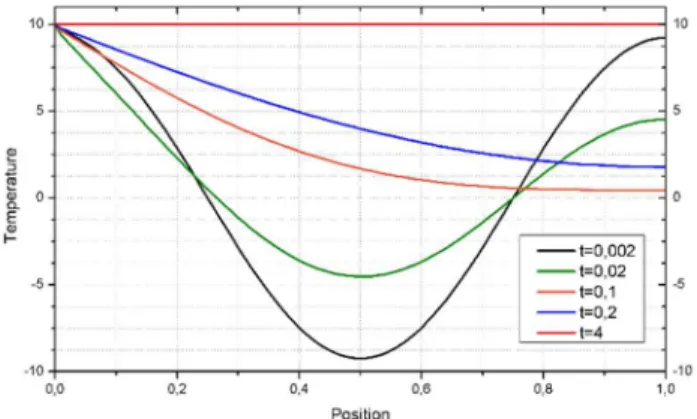
In this example, presented by Copetti (2002) is studied the thermal behavior of a one-dimensional bar with thermal loading. The bar was divided into 100 elements of equal size. The author adopts the thermal conductivity, the specific heat and the density of the material equivalent to 1. The temporal discretization is performed with a time interval equal to 0.0001.

The Figure 1 shows the thermal load along the bar, described by Equation:

( )

p x x ₍₅₂₎

The temperature and displacement are constrained at the position x =0:

( )

q t = ₍₅₃₎

( )

u t ₍₅₄₎

The Figures 1 and 2 give a summary of the temperature variations over time. The results obtained are similar to the Copetti (2002).

Figure 1: Temperature change.

As shown in Figure 1, because the boundary conditions the temperature of all nodes tend to remain in equilibrium when t = 4. It should be noted that over time the thermal load is dissipated

between the nodes. Figure 2 illustrates the path of the thermal balance for different positions of the bar, where they tend to a common point (q =10).

4.2 Temperature Evolution in a Rod

This example was originally presented by Kamlah and Haupt (1998), and subsequently by Carrazedo and Coda (2010), which consist in a cylindrical rod of 10cm length under elastoplastic loading and

a reference temperature of 293K , under the following initial and boundary conditions:

( )

q x = ₍₅₅₎

( )

(

)

q t =q t = ₍₅₆₎

The following material properties were set:

10 2

2 10

=

E kgf m k = 20 J

(

)

7800

r = kg m c_e = 480 J

(

)

7 2

2 10

s_Y = kgf m a= 0.000016 m

(

)

It considered the kinematic hardening, with a value of _{H =3 10}8_{kgf /m}2_{. It is assumed that all}

plastic work is converted into heat, or neglects to stored energy of cold work. An important consideration used by the authors is that the temperature does not cause deformations. Furthermore, the loading history is given by a non-monotonic strain history with changing absolute value of the strain rate:

( )

e_{ t = s}

-for 0 %£ £e 1.5 %  0 s£ £t 150 s

( )

e_{ t = - s}

-for 1.5 %£ £ -e 1.5 %  150 s£ £t 210 s

( )

e_{ t = s}

-for -1.5 %£ £e 1.0 %  210 s £ £t 335 s

With the aid of the mechanical model response, this process can be divided further in periods of elastic and elastoplastic loading:

1. 0 s£ £t 10 s Elastic tension

2. 10 s£ £t 150 s Elastoplastic tension

3. 150 s £ £t 154 s Elastic compression 4. 154 s£ £t 210 s Elastoplastic compression 5. 210 s£ £t 220 s Elastic tension

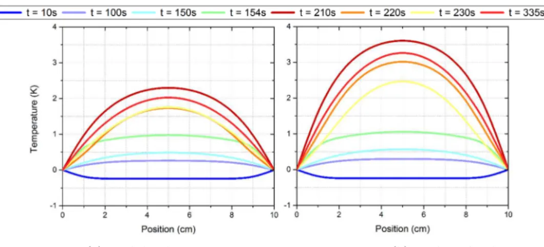
Confronting the results obtained with the work mentioned above. The different elastic and elastoplastic periods in the history of loading can be easily identified in Figure 3, which illustrates the thermomechanical heat source through time. It is noted that the elastoplastic hardening model has a heat source larger than the perfect elastoplastic model and therefore more relevant temperature changes. The Figure 4 shows the temperature variation in the center of rod.

Figure 3: Mechanical heat source.

Figure 4: Temperature variation in time.

(a) With hardening (b) Without hardening

The Figure 5 shows the temperature variation along the rod for different time instants. Changes in heating and cooling phases are defined by the state of the body changes. As expected, it is noted that the elastoplastic model with strain hardening kinematic presents higher temperature variations than the perfect elastoplastic model, due to the levels of stresses in the kinematic model are higher.

4.3 Impact of a Bar on a Rigid Wall

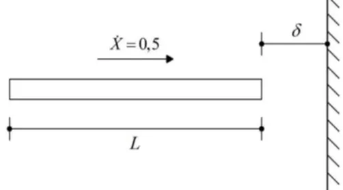
This example, approached initially by Armero and Petocz (1998), consists of uniaxial impact from a bar (with a constant velocity) and rigid wall, as shown in Figure 6. The problem is modified to consider the thermomechanical effects. The geometrical and material characteristics of both elements are given by: E =1, L =1, A=1, r =1, k =1, c_e =1, a=0.17 and d =0.05.

Figure 6: Impact of a rod on a rigid wall. Problem definition.

Only the extremity node of the bar is impacted. It is investigated the behavior of contact forces, velocities, stresses and temperature changes of the bar. In this example it is investigated only geometric nonlinearity. The time discretization is done to 250 time steps of 0.01. The bar is discretized with 20 finite elements of the same dimension.

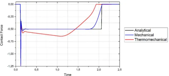
The Figures 7 and 8 describe respectively the velocity and contact force, comparing the analytical response to the mechanical and thermomechanical numeric responses. In both figures, before the impact, mechanical and thermomechanical response are equal and the structure does not show deformations.

Figure 8: Contact force on impact point.

The velocity results of mechanical and thermomechanical models of the impactor node are practically identical up to the instant of 1.93. After this time instant, the difference between the models increases with time. As shown in Figure 8, the heat generation resulting in higher contact forces to mechanical response, and consequently the contact time is reduced.

The Figure 9 shows the temperature field to the undeformed configuration of the bar. It is considered the coupled and the uncoupled problem, respectively. It is observed that the thermomechanical coupling causes a secondary effect and temperature variations were more relevant when considering that the temperature changes generate deformations. The bar has maximum temperatures between times instants of 1.0 and 1.5, approximatively. The bar begins to cool quickly after reflection.

(a) With hardening (b) Without hardening

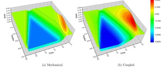
In the surface of Figure 10 it is possible to compare the stresses on the bar. It is observed a redistribution of stresses caused by thermomechanical coupling. In mechanical problem the stress varies between -0.50 and 0.20. While the problem coupled, has higher stress levels in compression and traction varying from -0.60 to 0.30. Consequently, the thermomechanical coupling increases the contact force and reduces the contact time.

(a) Mechanical (b) Coupled

Figure 10: Stress field over time and space.

4.4 Unidirectional Impact Between Two Bars

In this example it is studied the case of impact between two identical bars with the same initial velocity (Figure 11), however, moving in opposite senses. This example is present in the studies by Carpenter et al. (1991). The geometrical and physical characteristics of both elements are given by:

30000.0

=

E ksi,_{k =8.09 BTU ft h F( º )}-1_{, =0.120 ( º )}-1 e

c BTU lb F , _{r =7.337 10}-4 _{lb s}2_/in4_, 2

1.0

=

A in and b = 0.8.

Figure 11: Problem description for one dimensional impact example.

Figure 12: Impact of a rod on a rigid wall. Problem definition.

The bar was discretized in 20 finite elements and the initial distance between the bars is

0.002

d = in. Plasticity is considered in the analysis. Adopts the model of hardening isotropic

15000

=

K ksi with sY =10 ksi. The reference temperature is 68 ºF. The numeric responses are

obtained with time intervals of D =t 0.0000005 s.

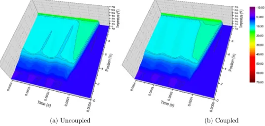
In Figure 13, verifies the plasticizing effect of heat generation at x =9.5in. It is observed that the evolution of temperature changes is very dependent on the accumulation of irreversible deformations. The Figures 14, 15 and 16 compare the temperature changes obtained with different coefficient of thermal expansion.

Figure 13: Hardening effect on the temperature changes (coupled).

(a) Uncoupled (b) Coupled

(a) Uncoupled (b) Coupled

Figure 15: Temperature field over time and space (a= 0.0000046).

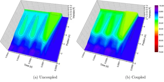
(a) Uncoupled (b) Coupled

Figure 16: Temperature field over time and space (a= 0.0000096).

It is noted that smaller coefficients of thermal expansion result in smaller temperature changes and small difference between the uncoupled and coupled responses. The thermomechanical coupled generates a secondary effect which causes larger variations in temperature and changes in the structural behavior.

The results presented in Figure 16 show high levels of temperature. In this case, due to redistribution efforts, the field of temperatures for coupled problem varies between -6.3 ºF and

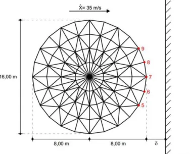
4.5 Impact Between a Plane Truss and a Rigid Wall

This example is the impact between a circular truss and rigid wall (Figure 17). The structure has 264 bars and 97 nodes. The time discretization is done through the Newmark method with

0.00001

D =t s. The geometrical and material data of both elements are given by:

11 2

2.1 10 /

=

E N m _{A=0.0036 m}2 _{H =5.0 10}8 _{N /m}2

27 / ( )

=

k J K m s _{s =1.0 10}8 _/ 2

Y N m ce = 480 J / (K kg) 3

7850 /

r = kg m a= 0.000011m/ (K m)

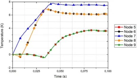
It is assumed that all plastic work is converted into heat. It adopts a reference temperature equivalent to 300K . The structure moves with velocity of 35m/s, with d = 0.01m .

Figure 17: Impact between a plane truss and a rigid wall. Problem definition.

Five nodes are impacted (Figure 17). The Figure 18 shows the evolution of temperature changes of the nodes impacting over time. The temperature of these nodes begin to increase rapidly from the moment of impact. It is observed a small decrease in the variations of temperatures from a certain moment, characterized by Gough-Joule effect and the dissipation of temperatures between nodes. The Figure 19 shows for different time, the temperature distribution of the structure in the deformed configuration.

Figure 18: Temperature change of impact points.

(a) t =0.01s (b) t =0.02s (c) t =0.04s

(a) t = 0.05s (a) t = 0.07s (a) t = 0.10s

5 CONCLUSIONS

A simple and effective alternative formulation to deal with the dynamic nonlinear systems, written in relation to nodal positions has been successfully applied to coupled thermomechanical problems. The formulation includes a complete treatment of the analysis of elastoplastic materials for simple configurations.

Through the numerical examples it is possible to observe the difference between the mechanical and the thermomechanical responses. Therefore, it is necessary to consider the interaction between thermal and mechanical behavior, which can cause redistributions of stress. The reference temperature is a determining factor in thermomechanical analysis, and high reference temperatures imply high temperature variations. The study of structures with elastoplastic behavior is important because depending on the history of deformation and accumulation of irreversible deformations, has a significant part in the generation of heat.

It emphasizes the consideration of thermomechanical coupling in impact problems, because the interaction between the mechanical and thermal response cause significant secondary effects due to high strain rates by modifying the structural behavior. Therefore, depending on the material, loading and initial conditions, the thermomechanical coupling can result in predominant contributions in structural response.

Acknowledgments

The authors would like to thank the Brazilian Research Funding Agencies CAPES (Coordination of Improvement of Higher Education Personnel), CNPq (National Council for Scientific and Technological Development) and FAPEMIG (Foundation for Research Support of Minas Gerais State) for the financial supports.

References

Armero, F., Petocz, E., (1998). Formulation and analysis of conserving algorithms for frictionless dynamic contact/impact problems. Computer Methods in Applied Mechanics and Engineering 158:269–300.

Benzerga, A. A., Brechet, Y., Needleman, A., Van der Giessen, E. (2005). The stored energy of cold work: Predictions from discrete dislocation plasticity. Acta Materialia 53:4765-4779.

Bever, M. B., Holt, D. L., Titchener, A. L. (1973). The stored energy of cold work. Mechanics of Materials 17:1-190. Biot, M. A. (1956). Thermoelasticity and irreversible thermodynamics. Journal of Applied Physics 27:240-253. Canadija, M., Brnic, J. (2004). Associative coupled thermoplasticity at finite strains with temperature-dependent material parameters. International Journal of Plasticity 20:1851-1874.

Canadija, M., Brnic, J. (2009). Nonlinear kinematic hardening in coupled thermoplasticity. Materials Science and Engineering A 499:275-278.

Canadija, M., Brnic, J. (2010). A dissipation model for cyclic non-associative thermoplasticity at finite strains. Mechanics Research Communications 37:510-514.

Carpenter, N. J., Taylor, R. L., Katona, M. G. (1991). Lagrange constraints for transient finite element surface contact. International Journal for Numerical Methods in Engineering 32:103-128.

Chen, J., Dargush, G. F. (1995). Boundary element method for dynamic poroelastic and thermoelastic analyses. International Journal of Solids and Structures 32:2257-2278.

Clayton, J. D. (2013). Nonlinear eulerian thermoelasticity for anisotropic crystals. Journal of the Mechanics and Physics of Solids 61:1983-2014.

Coda, H. B., Greco, M. (2004). A simple FEM formulation for large deflection 2D frame analysis based on position description. Computer Methods in Applied Mechanics and Engineering 193:3541-3557.

Coda, H. B., Paccola, R. R. (2008). A positional FEM formulation for geometrical non-linear analysis of shells. Latin American Journal of Solids and Structures 5:205-223.

Coda, H. B., Paccola, R. R. (2011). A FEM procedure based on positions and unconstrained vectors applied to non-linear dynamic of 3D frames. Finite Elements in Analysis and Design 47:319-333.

Coda, H. B., Paccola, R. R., Sampaio, M. S. M. (2013). Positional description applied to the solution of geometrically non-linear plates and shells. Finite Elements in Analysis and Design 67:66-75.

Copetti, M. I. M. (1999). Finite element approximation to a contact problem in linear thermoelasticity. Mathematics of computation 68:1013-1024.

Copetti, M. I. M. (2002). A one-dimensional thermoelastic problem with unilateral constraint. Mathematics and Computers in Simulation 59:361-376.

Danilovskaya, V. (1950). Thermal stresses in an elastic half-space due to sudden heating of its boundary. Prikl. Mat. Mech. 14:316-324.

Dargush, G. F., Banerjee, P. K. (1991). Boundary element methods for three-dimensional thermoplasticity. International Journal of Solids and Structures 28:549-565.

Deb, A., Henry Jr., D. P., Wilson, R. B. (1991). Alternative BEM formulations for 2- and 3-D anisotropic thermoelasticity. International Journal of Solids and Structures 27:1721-1738.

Dillon Jr., O. W. (1963). Coupled thermoplasticity. Journal of the Mechanics and Physics of Solids 11:21-33.

Farren, W. S., Taylor, G. I. (1925). The heat developed during plastic extension of metals. Proceedings of the Royal Society of London 107:422-451.

Greco, M., Coda, H. B., Venturini, W. S. (2004). An alternative contact/impact identification algorithm for 2d structural problems. Computational Mechanics 34:410-422.

Greco, M., Coda, H. B. (2006). Positional FEM formulation for flexible multi-body dynamic analysis. Journal of Sound and Vibration 290:1141-1174.

Greco, M., Ferreira, I. P., Barros, F. B. (2013). A classical time integration method applied for solution of nonlinear equations of a double-layer tensegrity. Journal of the Brazilian Society of Mechanical Sciences and Engineering 35:41-50.

Greco, M., Gesualdo, F. A. R., Venturini, W. S., Coda, H. B. (2006). Nonlinear positional formulation for space truss analysis. Finite Elements in Analysis and Design 42:1079-1086.

Greco, M., Menin, R. C. G., Ferreira, I. P., Barros, F. B. (2012). Comparison between two geometrical nonlinear methods for truss analyses. Structural Engineering and Mechanics 41:735:750.

Green, A. E., Lindsay, K. A. (1972). Thermoelasticity. Journal of Elasticity 2:1-7.

Green, A. E., Naghdi, P. M. (1993). Thermoelasticity without energy dissipation. Journal of Elasticity 31:189-208. Green, A. E., Naghdi, P. M. (1995). A unified procedure for construction of theories of deformable media. I – Classical continuum physics, II – Generalized continua, III – Mixtures of interacting continua. Proceedings of the Royal Society: Mathematical, Physical & Engineering Sciences 448:335-388.

Kamlah, M., Haupt, P. (1998). On the macroscopic description of stored energy and self heating during plastic deformation. International Journal of Plasticity 13:893-911.

Kapoor, R., Nemat-Nasser, S. (1998). Determination of temperature rise during high strain rate deformation. Mechanics of Materials 27:1-12.

Kolupaeva, S., Semenov, M. (2015). The stored energy of plastic deformation in crystals of face-centered cubic metals. Materials Science and Engineering 71:1-6.

Lemonds, J., Needleman, A. (1986). Finite element analyses of shear localization in rate and temperature dependent solids. Mechanics of Materials 5:339-361.

Li, X. (1992). A generalized theory of thermoelasticity for an anisotropic medium. International Journal of Engineering Science 30:571-577.

Lord, H. W., Shulman, Y. (1967). A generalized dynamical theory of thermoelasticity. Journal of the Mechanics and Physics of Solids 15:299-309.

Lu, S. C. H., Pister, K. S. (1975). Decomposition of deformation and representation of the free energy function for isotropic thermoelastic solids. International Journal of Solids and Structures 11:927-934.

Lubarda, V. A. (2004). Constitutive theories based on the multiplicative decomposition of deformation gradient – Thermoelasticity, elastoplasticity, and biomechanics. ASME Applied Mechanics Review 57:95-108.

Lychev, S. A., Manzhirov, A. V., Joubert, S. V. (2010). Closed solutions of boundary-value problems of coupled thermoelasticity. Mechanics of Solids 45:610-623.

Mahmoud, W., Ghaleb, A. F., Rawy, E. K., Hassan, H. A. Z., Mosharafa, A. A. (2015). Numerical solution to a nonlinear, one-dimensional problem of anisotropic thermoelasticity with volume and heat supple in a half-space – interaction of displacements. Archive of Applied Mechanics 85:433-454.

McKnight, R. L., Sobel, L. H. (1977). Finite element cyclic thermoplasticity analysis by the method of subvolumes. Computers and Structures 7:417-424.

Mroz, Z., Oliferuk, W. (2002). Energy balance and identification of hardening moduli in plastic deformation processes. International Journal of Plasticity 18:379-397.

Nickell, R. E., Sackman, J. L. (1968). Approximate solutions in linear coupled thermoelasticity. Journal of Applied Mechanics 35:255-266.

Norris, A. N. (2006). Dynamics of thermoelastic thin plates – a comparison of four theories. Journal of Thermal Stresses 29:169-195.

Oliferuk, W., Swiatnicki, W. A., Grabski, M. W. (1993). Rate of energy storage and microstructure evolution during the tensile deformation of austenitic steel. Materials Science and Engineering A 161:55-63.

Ozakin, A., Yavari, A. (2010). A geometric theory of thermal stresses. Journal of Mathematical Physic 51:1-32. Perzyna, P., Sawzcuk, A. (1973). Problems in thermoplasticity. Nuclear Engineering and Design 24:1-55. Rajagopal, K. R. (1995). Boundary layers in finite thermoelasticity. Journal of Elasticity 36:271-301.

Rajagopal, K. R., Maneschy, C. E., Massoudi, M. (1996). Inhomogeneous deformations in finite thermos-elasticity. International Journal of Engineering Science 34:1005-1017.

Rand, O., Givoli, D. (1995). Reduction of the periodic thermoelastic deformation in truss-structures by design refinements and active loads. Computers and Structures 54:757-765.

Reis, M. C. J., Coda, H. B. (2014). Physical and Geometrical non-linear analysis of plane frames considering elastoplastic semi-rigid connections by the positional FEM. Latin American Journal of Solids and Structures 11: 1163-1189.

Rittel, D., Kidane, A. A., Alkhader, M., Venkert, A., Landau, P., Ravichandran, G. (2012). On the dynamically stored energy of cold work in pure single crystal and polycrystalline copper. Acta Materialia 60:3719-3728.

Rosakis, P., Rosakis, A. J., Ravichandran, G., Hodowany, J. (2000). A thermodynamic internal variable model for the partition of plastic work into heat and stored energy in metals. Journal of the Mechanics and Physics of Solids 48:581-607.

Sampaio, M. S. M., Paccola, R. R., Coda, H. B. (2015). A geometrically nonlinear FEM formulation for the analysis of fiber reinforced laminate plates and shells. Composite Structures 119: 799-814.

Serra, E., Bonaldi, M. (2009). A finite element formulation for thermoelastic damping analysis. International Journal for Numerical Methods in Engineering 78:671-691.

Shahani, A. R., Bashusqeh, S. M. (2014). Analytical solution of the thermoelasticity problem in a pressurized thick-walled sphere subjected to transient thermal loading. Mathematics and Mechanics of Solids 19:135-151.

Shahani, A. R., Nabavi, S. M. (2007): Analytical solution of the quasi-static thermoelasticity problem in a pressurized thick-walled cylinder subjected to transient thermal loading. Applied Mathematical Modelling 9:1807-1818.

Sherief, H. H., Hamza, F. A., Saleh, H. A. (2004). The theory of generalized thermoelastic diffusion. International Journal of Engineering Science 42:591-608.

Simo, J. C., Miehe, C. (1992). Associative coupled thermoplasticity at finite strains: Formulation, numerical analysis and implementation. Computer Methods in Applied Mechanics and Engineering 98:41-104.

Simo, J. C., Wriggers, P., Schweizerhof, K. H., Taylor, R. L. (1986). Finite deformation post-buckling analysis involving inelasticity and contact constraints. International Journal for Numerical Methods in engineering 23:779-800.

Siqueira, T. M., Coda, H. B. (2016). Development of sliding connections for structural analysis by a total lagrangian FEM formulation. Latin American Journal of Solids and Structures 13:2059-2087.

Soler, A. L., Brull, M. A. (1965). On solution to transient coupled thermoelastic problems by perturbation techniques. Journal of Applied Mechanics 32:389-399.

Stanley, P. (2008). Beginnings and early development of thermoelastic stress analysis. Journal Compilation 44:285-297. Taylor, G. I., Quinney, H. (1934). The latent energy remaining in a metal after cold working. Proceedings of the Royal Society: Mathematical, Physical and Engineering Sciences 143:307-326.

Ting, E. C., Chen, H. C. (1982). A unified numerical approach for thermal stress waves. Computers and Structures 15:165-175.

Vujosevic, L., Lubarda, V. A. (2002). Finite-strain thermoelasticity based on multiplicative decomposition of deformation gradient. Theoretical and Applied Mechanics 28-29:379-399.

Wong, M. B., Tin-Loi, F. (1990). Geometrically nonlinear analysis of elastic framed structures. Computers and Structures 34:633-640.

Yavari, A., Goriely, A. (2013). Nonlinear elastic inclusions in isotropic solids. Proceedings of the Royal Society: Mathematical, Physical and Engineering Sciences 469:1-21.