Predictive analysis in healthcare

(1)

Department of Information Science and Technology

Predictive analysis in Healthcare

Filipe da Silva Gonçalves

Dissertation submitted as partial fulfillment of the requirements for the degree of Master in Computer Engineering

Supervisor:

Doctor Rúben Filipe de Sousa Pereira, Assistant Professor, ISCTE-IUL

Co-supervisor:

Doctor João Carlos Amaro Ferreira, Assistant Professor, ISCTE-IUL

(2)

i

Acknowledgements

There are several persons that were important during the journey of development of this master’s thesis.

Firstly, I would like to express my gratitude towards my thesis advisors, Dr. Rúben Pereira and Dr. João Ferreira for the constant and valuable reviews of my work, guiding me through the research and development processes and helping me to improve it through quality feedback. I am humbled and thankful for all of your effort. I would also like to express my gratefulness to the management of the hospital that collaborated with me through the development of the thesis, for promptly providing me with any of the needed resources.

As a student-worker I would also like to thank everyone in my workplace, specially Ana Lara, João Andrade, Fábio Costa and Diogo Pires for all the support, both motivational and technical. You were some of the pillars of this journey, helping me when I needed.

Finally, I also want to show my appreciation towards my family and close friends for the unconditional love and for providing me with all the conditions needed to complete this important step in my life.

(3)

(4)

iii

Resumo

As urgências dos hospitais são o maior ponto de entrada para o sistema de saúde. Com o aumento da esperança média de vida e o aumento do número de doenças, aumentou a necessidade e a procura dos serviços de saúde, levando a que seja importante que as urgências dos hospitais consigam fazer uma gestão eficiente dos seus recursos de forma a proporcionar a melhor experiência possível aos seus utentes. Se a procura por recursos nas urgências dos hospitais for superior aos recursos disponíveis, ocorre um fenómeno de concentração excessiva de pessoas nas urgências, o que pode causar vários problemas como por exemplo tempos de espera mais longos, falta de camas, utentes nos corredores, o que acaba por afetar a satisfação dos utentes.

Uma forma de aumentar a satisfação dos utentes é através da previsão do tempo de espera nas urgências do hospital, visto que ajuda a administração do hospital a fazer uma melhor gestão dos recursos disponíveis e oferecer uma previsão do tempo de espera aos utentes leva a maior satisfação.

O autor desenvolveu em conjunto com um hospital Português perto de Lisboa, usando dados reais, um protótipo que permite fazer a previsão do tempo de espera nas urgências do hospital. Para complementar os dados providenciados pelo hospital, o autor adicionou alguns atributos como informação do estado meteorológico por dia (temperatura, humidade, precipitação e vento), anúncios da Direção-Geral de Saúde (DGS) e o número de jogos de futebol das duas principais equipas de Lisboa (Sporting CP e SL Benfica) por dia.

O autor aplicou os algoritmos Naive Bayes e Random Forest em três cenários diferentes: o primeiro em que apenas se utilizam os dados originais providenciados pelo hospital, o segundo em que se adicionam os atributos dos anúncios da DGS e o número de jogos de futebol e o terceiro em que para além dos atributos do cenário anterior, se adicionou os atributos relativos ao estado meteorológico do dia mencionados anteriormente.

O algoritmo com melhor performance foi o Random Forest, principalmente no terceiro cenário, fator que levou a que este tenha sido o modelo escolhido para ser utilizado no protótipo. Depois de fazer as previsões do tempo de espera e analisar os resultados, pode- se concluir que para além do algoritmo Random Forest apresentar melhores resultados para a previsão do tempo de espera nas urgências, tendo em conta o tipo de dados

(5)

iv fornecido, os atributos externos adicionados posteriormente e que não pertenciam ao conjunto de dados original providenciado pelo hospital, não são dos atributos que mais afetam os tempos de espera, sendo que os atributos que têm mais importância para os tempos de espera das urgências são a cor de triagem e a categoria da doença.

Palavras-Chave: Urgências hospitalares; Previsão de tempos de espera; Cuidados de

(6)

v

Abstract

The Emergency departments (ED) are the major entry point to the healthcare system. With the growing demand due to the increase of life expectancy and the greater number of diseases, it is mandatory for the ED’s to have a more efficient resource management in order to try and provide the best experience possible to its patients. If the resource demand is greater than the resources available, then ED crowding occurs. This phenomenon leads to several problems that affect the patient experience, like longer waiting times, lack of beds, patients in hallways, etc.

One of the ways to improve patient satisfaction is through patient waiting time prediction, since it would allow for a better resource management in the ED and providing patients with a waiting time estimation on the triage increases patient satisfaction. The author collaborated with a Portuguese hospital near Lisbon using real ED data and built a prototype to predict the ED waiting time. The researcher complemented the ED original dataset with external data like weather information, DGS Announcements and number of football games, to try to find the most accurate model.

To perform the prediction, the Naïve Bayes (NB) and Random Forest (RF) algorithms were applied in three different scenarios: the first one only with data from the original dataset, the second one where the number of football games and DGS announcements attributes were added and finally, a third one with the same dataset as the previous scenario but added weather information (temperature, wind, humidity and precipitation). The RF algorithm was the one with the best performance, especially in the third scenario. For this reason, the author used the RF algorithm with the variable inputs from the third scenario to perform the predictions on the prototype. The author concluded that the external data attributes added in both second and third scenarios were not the most important attributes for the waiting times, being the most important variables, the triage colors, disease category.

Keywords: emergency department; waiting time prediction; healthcare; big data; patient

(7)

(8)

vii

List of Tables

Table 1 - Manchester Triage Protocol ... 15

Table 2 - Waiting time discretized classes ... 21

Table 3 - Period of the day discretized classes ... 21

Table 4 - Average waiting times per triage color ... 25

Table 5 - Average waiting time per period of the day class ... 27

Table 6 - Top five disease categories with the longest average waiting time ... 28

Table 7 - Possible values for the attributes used as input for the applied algorithms .... 35

Table 8 - Top 3 variables with the highest probability for each patient waiting time .... 39

Table 9 - Accuracy for each predicted class with Naive Bayes algorithm ... 41

Table 10 - Performance results of the Naive bayes algorithm ... 42

Table 11 - Classification error values for each of the waiting time classes ... 43

Table 12 - Performance results of the RF algorithm ... 44

(11)

(12)

xi

List of Figures

Fig 1- Methodology processes performed during this research ... 13

Fig 2 - ED flow followed in the studied hospital ... 14

Fig 3 - Population age distribution according to the Portuguese 2011 Census ... 15

Fig 4 - Original dataset attributes list ... 17

Fig 5 - Attributes used during the research... 23

Fig 6 - Average waiting time distribution through a day of the week ... 26

Fig 7 - Average waiting time per period of the day... 26

Fig 8 - Percentage of records per triage color ... 28

Fig 9 - Monthly distribution of "Diseases of the respiratory system." ... 29

Fig 10 - Prototype schema ... 31

Fig 11 - Variables used in the dataset to apply the algorithms ... 33

Fig 12 - Variables used in applying the algorithms in Scenario 1. ... 36

(13)

(14)

xiii

List of abbreviations and acronyms

ACEP - American College of Emergency Physicians DGS - Direcção Geral da Saúde

ED - Emergency Department EHR - Electronic Health Records F1 - F1-Score

GDPR - General Data Protection Regulation IF - Impact factor

ICD9 - International Classification of Diseases 9 KPI - Key performance indicator

MTP - Manchester Triage Protocol NB - Naïve Bayes

PA - Predictive Analytics PREC - Precision

RF - Random Forest TPR - True-Positive rate

(15)

1

Chapter 1 – Introduction

Emergency departments (ED) are an important and complex area of a hospital and are the major entry point to the healthcare system [1]. With the increase in life expectancy, population ageing and a larger amount of health issues, ED tends to have higher demand [2]. If hospitals and more specifically, ED, are not ready, this will increase emergencies crowding, creating a big problem for authorities and hospital management since resources are limited [2]. According to the American College of Emergency Physicians (ACEP) “Crowding occurs when the identified need for emergency services exceeds resources for patient care in the emergency department, hospital or both” [3]. Lack of beds, patients in hallways, a greater amount of people in the waiting rooms, longer waiting times, greater patient length of stay and general patient dissatisfaction are some of the consequences of this phenomenon. It is an international problem, and it is vital for hospitals to solve it due to the life-threatening context of the area [3].

ED wait times are the second most referred theme regarding patient experience [4] which indicates that this area requires intervention to increase care quality and resource efficiency to achieve greater patient satisfaction. That can be achieved using Predictive Analytics (PA) which has the potential to improve the operational flexibility and throughput quality of ED services [5]. Waiting time prediction would help clinicians prioritize patients and adjust workflow to minimize the time spent [6].

Predictive Analytics allows predicting future events or trends using retrospective and current data [7]. It could be applied in several healthcare areas, taking advantage of the big data in healthcare.

Big data refers large volumes of high velocity, complex and variable data that require advanced techniques and technologies to enable the capture, storage, distribution, management and analysis of the information as stated in [8] based on a report delivered to the U.S Congress in 2012.

The complexity associated with big data is due to its dimensions velocity, variety, and volume [9]. In the healthcare industry, there is another critical dimension which is veracity [8]. The data for healthcare needs to be veracious so that the decisions can be as accurate as possible since sometimes those decisions can mean life or death of the patient. Some authors defend the inclusion of other dimensions like value [10], validity or volatility [11].

(16)

2 Big Data in healthcare can be overwhelming not only due to the volume dimension but also because of the variety of sources from where it is collected and the speed at what it must be managed [8], especially if the goal is to apply real-time analytics. Part of the data used in big data healthcare analytics comes from electronic health records (EHR) which are real-time databases of patient health information including medical history, diagnoses, medications, allergies, lab tests, etc [12]. Other sources can be clinical decision support systems, government sources, laboratories, pharmacies or insurance companies [8].

With technological advances, newer sources are becoming available like 3D imaging, genomics and biometric sensors [8]. However, this variety of sources are challenging since some of them are unstructured, do not use a homogeneous format [12]. Using this data, analytics can be performed, extracting knowledge by discovering patterns on that data [13]. This knowledge allows going for evidence-based medicine. Performing big data analytics in healthcare would allow to know new diseases and treatments, predict treatment outcomes, support real-time decisions, disease surveillance, control outbreaks, manage population health, etc. [10].

An example where big data analytics was applied with success is at the Johns Hopkins School of Medicine where Google Flu Trends data is used to predict sudden increases in flu-related emergency room visits earlier. Another example comes from the Columbia University Medical Center where analytics are used to provide clinicians with critical information to help treating complications in patients with brain injuries [8]. There are several big data analytics techniques like statistical modeling, artificial intelligence, predictive analytics, data mining, and machine learning techniques [14]. According to [13], one tactic that healthcare organizations should adopt is the more effective use of predictive analytics, allowing the stratification of risk to predict outcomes and in healthcare, outcomes can be harmful to the patients.

Some of the advantages of applying predictive analytics in healthcare would be the adoption of more sensor-based technologies, provide lifestyle changes suggestions [14], help the management of high risk and high-cost patients [13], improve resource management, readmissions prevention, complications estimation at triage, etc.

Grounded on the aforementioned points, this research describes the application of data mining techniques using data collected from a Portuguese hospital ED. This dataset was supplemented with other external data attributes like weather information and national announcements. With this, the author aimed to help hospital’s management to improve

(17)

3 the quality of their service, giving them more insights about the waiting times and diseases behavior regarding some dimensions that will be forwardly identified, allowing them increase patient satisfaction [15].

1.1. Goals

During this research, the author aims at predicting the patient ED waiting time, by building a prototype that based on an input, produces an output that represents an estimation of patient waiting time. The author applied data mining techniques with different input configurations and compared its performance in order to find the most accurate model for the core of the prototype. Throughout the research, the author also seeks to discover the Key Performance Indicators (KPI’s) regarding the emergency department waiting time. This prototype can be used by different interactors, both patients, to understand the waiting times in the ED of the hospital, or the hospital ED management to understand the current or future status of the ED waiting times and ensure correct resource management. This allows for more efficient resource management and greater patient satisfaction [15].

1.2. Thesis Organization

The rest of the document is organized in six different sections. First, the Chapter 2: Literature review and Related work, which is subdivided on four where big healthcare data availability and problems are analyzed, as well as predictive analytics in healthcare, focusing on the ED waiting times and procedures. Then, Chapter 3: Work Methodology, where the work methodology followed during this research is explained, introducing the four main sub-processes involved. The next section, Chapter 4: Data Pre-processing where inconsistent data was removed, and new external data (weather information, number of football games and announcements regarding public health) was added to complement the dataset. Then, Chapter 5: Statistical Analysis, which corresponds to the section where some analysis were performed in order to gain more insights about the data. After, Chapter 6: Predictive Analytics through a Data Mining approach, where data mining techniques were applied to the dataset with the goal of predicting the patient waiting time and understand the main factors that influence it. Finally, the last section,

(18)

4 Chapter 7: Conclusions, where the results are analyzed and compared with the predefined goals of the research.

(19)

5

Chapter 2 – Literature Review and Related Work

The goal of this master thesis is to study the emergency waiting times, applying predictive analytics and investigating the main factors that influence the ED waiting time, to build a prototype of a system that allows predicting ED waiting time, for a Portuguese hospital near Lisbon.

To achieve this, the author started by researching big data analytics in healthcare, learning about the data diversity of the area and analyzing examples of predictive analytics applications. Later on, the focus was shifted to researching the ED waiting times, to understand which were the most important factors regarding the ED waiting time as well as the best data mining approaches. Each one of these steps represents one sub-section on this chapter.

The research was conducted on IEEE digital library, ACM digital library, SpringerLink, ResearchGate and ScienceDirect, using the keywords “Big data analytics in healthcare”, “Predictive analytics in healthcare”, “Predictive analysis in healthcare”, “Predictive analytics in Emergency Department” and “Emergency Department waiting time prediction”.

2.1. Big Data Analytics in Healthcare

Most of the authors in this section produced a framework or a model on how to apply big data analytics in healthcare. For example, Chauhan and Jangade [14] propose an architectural framework for big data analytics in healthcare, studying tools, data mining techniques and data sources. Some of those authors also explained big data characteristics in healthcare, based on Gartner 2012, that defended that there are three main big data characteristics, volume, velocity and variety. Some of those authors are Kankanhalli et al. [9], who studied on how big data analytics can be applied in the healthcare industry, defending that it has three main characteristics: volume, velocity and variety. They described the new data sources like medical images, sensor data, genomics, etc. The authors defend that predictive analytics will be “the next revolution both in statistics and medicine around the world”.

W. Raghupathi and V. Raghupathi [8] also studied big data analytics in the healthcare industry, but added a new characteristic for big healthcare data, which is

(20)

6 veracity. The authors defined big data in healthcare as “electronic health data sets so large and complex that they are difficult (or impossible) to manage with traditional software and/or hardware”. They have studied some of the existent challenges like the new data sources and unstructured data and some of the possible benefits in areas like early detection of diseases, general population health management, treatment outcome prediction or risk for medical complications. Finally, provided an architectural framework on how to apply big data analytics in healthcare, analyzing different tools and methodologies.

Asri et al. [10] defend that big data in healthcare has the same characteristics as described by W. Raghupathi and V. Raghupathi [8], adding value as a new characteristic. The authors studied the application of big data in healthcare, giving the example of reality mining, which can be defined as “using big data to study our behavior through mobile phone sensors” and how it can be used in healthcare. The research also explores some of the big data analytics challenges like data sources, data quality and human resources needed to implement and manage big data analytics systems and how it can help patients, clinicians and researchers.

Ojha and Mathur [11] proposed the application of big data analytics in an Indian Hospital and when characterizing big data in healthcare, added two new characteristics to the idea of W. Raghupathi and V. Raghupathi [8], validity and volatility. They defined big data as “extremely large data sets that can be analyzed computationally to find patterns, trends, and associations, visualization, querying, information privacy and predictive analytics on large wide spread collection of data.” exploring the advantages and limitations of its usage. Also defined EHR as “systematic collection of patient’s electronic health information which can be shared across different units of the hospital through a connected network”.

Others did not propose a framework but studied how big data could be applied in healthcare, pointing out challenges and possible benefits.

One of those authors is Dinov [7] who studied how big data can be applied in healthcare, pointing out its challenges like different data formats, unstructured data, incompleteness and data complexity, and explaining benefits and possible usages like predictive analytics. Compared algorithms and methods that can be used in healthcare.

(21)

7 Others are Reddy and Kumar [16] that also discussed how big data analytics could be beneficial to the healthcare industry, reviewing and comparing tools and techniques.

Other authors, focused on some specific areas, like Bates et al. [13] that studied how big data analytics can be applied in healthcare, more specifically in high risk and high-cost patients management, or Belle et al. [17] that focused on medical image processing, signal processing and genomics, pointing challenges, tools and algorithms (for example SVM) to be applied.

Palem [12] focused on data sources and studied how EHR and Clinical decision support systems (CDSS) can be beneficial to the healthcare industry, discussing its benefits and challenges like data privacy and unstructured data.

2.2. Predictive Analytics in Healthcare

Some authors reviewed and applied predictive analytics in the healthcare industry, studying its advantages and possible applications, like Malik et al. [18] that reviewed and analyzed applications of predictive analytics and data mining in the healthcare industry.

Chauhan and Jangade [14] claim that predictive analytics in healthcare can be beneficial as it would allow for patient disease prediction, fraud detection and cost management initiatives.

Another author that defends predictive analytics importance in the healthcare industry is Palem [12], defending that predictive analytics can be helpful on various areas of the healthcare industry like “life-sciences, healthcare providers, insurance providers, public health, individuals”.

For Janke et al. [5] predictive systems can also be beneficial to the ED. They studied big data and predictive analytics implementation challenges and opportunities and how it could improve the ED patient flow, also analyzing several algorithms that can be used to apply predictive analytics in healthcare.

The aforementioned systems or models are defined by Kaul et al. [19], that defined predictive models as models that “concentrate upon analyzing a set of relevant data, and predict a future implication or a meaningful pattern” and analyzed how they can be applied in healthcare, for example, allowing to provide alerts about disease outbreaks. They have studied healthcare data and state that “80% of medical data is unstructured and

(22)

8 difficult to analyze”. Compared the usage of three different algorithms (CARE, COHESY, and HARM) to be applied in a predictive system.

To help the community using predictive analytics, Qureshi [20] proposed a framework to apply Predictive Analysis in healthcare, based on cloud computing, allowing institutions from different areas to collaborate (insurance companies, hospitals, research centers, etc).

Soni and Vyas [21] compared some associative classifiers and classification techniques to be applied on predictive analytics in healthcare, stating that associative classifiers have the advantage of being easier to interpret and the dataset can be updated without major consequences unlike other traditional algorithms like decision trees.

Chennamsetty et al. [22] developed a system that allows performing predictive analysis, which will help on patient treatment, by analyzing several patient characteristics like “family history, lifestyle, smoking habits “. This system was built using the tool Hive and is based on the management of EHR, which can be defined as a “digital version of a patient’s medical chart”. During the development of this system, the authors analyzed the challenges regarding the usage of EHR as well as the possible benefits, claiming that it allows to “improve safety, quality, the efficiency of healthcare”.

Some of the authors also analyzed the advantages of predictive analytics but focusing on some specific areas. One of those cases is Bates [13] that provided some use cases of predictive analytics application on high risk and cost patient management. They also defined predictive systems as “software tools that allow the stratification of risk to predict an outcome”, defending that, in the future, healthcare organizations will use predictive analytics.

Alharbey [23] created a model to predict exacerbations of patients that suffer from Chronic Obstructive Pulmonary Disease (COPD) based on Neural Network with backpropagation algorithm. With this system care givers could provide early care avoiding possible negative outcomes.

Behara et al. [24] developed a model to predict the outcome of diabetes occurrence. Used multi-layer perceptron (MLP) and Bayesian networks as classifiers with the help of the tool Weka.

One of the areas that were most analyzed was the ED. According to Fong et al. [25], the “emergency department has been recognized as one of the most interruption laden

(23)

9 environments”. The authors developed a model to predict if a clinician will return to its task after an interruption, using logistic regression, defining memory decay from the interruption and workload during the interruption as main factors for task resumption.

2.3. ED Procedures and Waiting times

As stated before, ED crowding is an important issue to solve, so Barad et al. [3] studied the ED of an Israeli hospital in order to find the reasons for ED crowding. Conducted interviews with the clinicians and analyzed the communication between departments. Used the American College of Emergency Physicians definition of ED crowding, “Crowding occurs when the identified need for emergency services exceeds resources for patient care in the emergency department, hospital or both”.

Khalifa [26] also studied the factors (input and throughput) that could affect ED crowding, also studying the ED crowding effects: “adverse clinical outcomes, reduced healthcare quality, impaired access to care and healthcare provider losses”. Used descriptive analytics methods in an ED of a Saudi Arabian hospital, suggesting the adoption of the CTAS – Canadian Triage and Acuity Scale – to filter the patients.

According to Liu et al. [1], the hospital capacity and the doctor behavior are some of the factors that have the most influence on the patient Length of Stay (LoS), which can affect ED Crowding. These authors, simulated an ED using agent-based simulation, to understand the relation between some of the ED sub-processes and the general state of the emergencies.

Regarding the patient LoS and its waiting times, in the United Kingdom, ED is required to ensure that “at least 98% of patients are discharged or admitted within 4 hours of arrival” [27].

2.4. Predictive analytics for ED waiting times

There are a few predictive analytics applications in the ED focusing on predicting the ED waiting times.

Some authors developed models using system simulation techniques, like Bruballa et al. [2] that created an agent-based simulation to study the patient length of stay, considering it as “one of the most important problems for the management of the

(24)

10 healthcare system worldwide”. They also defend that the existence of information or a recommendation system showing emergency department state information would help to avoid long waiting times in the services or Chong et al. [28] that developed a dynamic system model to study the patient flow in the emergency department of a hospital in Hong Kong. They concluded that by increasing staff and the number of beds, the time spent by patients in the ED could be reduced.

Others used machine learning techniques, like quantile regression, Q-Lasso or expectation maximization.

Sun et al. [6] were some of the authors that used quantile regression to develop a model to predict emergency department waiting time, based on triage information. Did not use the predicted mean waiting time since it is affected by possible outliers, instead, predicted “a range of the 50th_{percentile to the 95}th_{percentile”. They defined waiting time as the} “interval from triage end time to the physician’s consultation time” and considered that the patient flow rates of other acuity levels could impact on other levels since clinicians could move between queues. The inputs of the model were the patient flow rate in the last hour, the day of the event, start time and end time of the triage and patient acuity. This developed model ignored patient characteristics which could be a limitation. Other authors that used quantile regression were Ding et al. [15], that created a system to predict the length of stay in ED. They claim that “providing patients with an expected LoS at triage may result in increased patient satisfaction”. They considered three phases for the length of stay: waiting time, treatment time and boarding time, and used “acuity level, arrival day and time, arrival mode, chief complaint and patient characteristics.” as variables.

Q-Lasso was used by Ang et al. [29] to predict ED waiting time. They defined Q-Lasso as an algorithm that is a combination of the “queueing theory and the lasso method, that uses a penalty to correct estimation errors”. Data from four different hospitals from the United States of America was used, and the input variables of the model were the number of patients in the ED, number of patients of low-acuity that started treatment in within the last hour, time of the day and the week.

Wang et al. [27] used the expectation maximization algorithm in order to analyze long LoS of patients in ED in hospital in the United Kingdom.

(25)

11 Marshall and McCrink [30] modeled patient waiting times using a discrete conditional phase-type model. These models have two components, “one for continuous survival distribution and one for the inter-related variables”. They used logistic regression as the statistical approach for this last component. They considered two different types of waiting times: waiting time for treatment and waiting time for admission.

Sonis et al. [4] developed a systematic review of the literature about the emergency department patient experience. Analyzed several articles to understand which themes were more common. Concluded that communication, wait times and staff empathy were the most frequent themes when talking about the patient experience.

(26)

(27)

13

Chapter 3 – Work Methodology

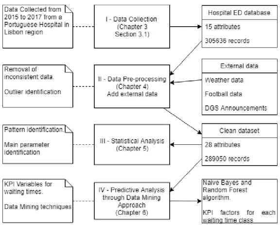
This section explains the work methodology followed in this research, which is summarized in Fig. 1. On this figure, the cards on the left represent a general description of what was achieved on the correspondent process, while the cards in the middle correspond to the name of each event. Finally, the cards on the right, represent the inputs for each process, the arrows meaning the flow of those aforementioned inputs.

The research started by the collecting data process, where hospital’s ED data, from 2015 to 2017 was extracted, counting with 3056363 event records each one with 15 attributes. Then, the data was processed, where inconsistent data and outliers were removed, and attributes from external sources were added in order to complement the dataset. This led to a clean and more complete dataset that didn’t have any outliers or inconsistent data and had 289050 event records with 28 attributes. This dataset was later used for statistical analysis, a process where the goal was to analyze and statistically understand the data. The clean dataset was also used for the last process, called Predictive Analysis through a Data Mining approach, which aimed at producing a prototype after identifying the main KPI’s for the waiting times and testing several input formulas with the Naïve Bayes and Random Forest algorithms.

(28)

14

3.1. Data Collection

On this process, the data used for the research was collected. This occurred between January 1st,_{2015 and December 31}st,_{2017 (a total of 1095 days), with data from a real} ED of a Portuguese hospital near Lisbon. Every time a patient visits the ED, a record is stored in the hospital’s internal database. In total there were 305 636 records, with each record representing the interaction of a patient with the hospital ED, containing a total of 15 attributes to describe it. These attributes are represented in Fig. 4 and will be explained after.

Whenever a patient visits the ED, a sequence of processes is followed, called the ED flow. The ED flow of this ED has five main processes. It starts with the patient admission, that corresponds to the process where the patient is admitted to the ED. The next process is the triage, where the patient will be assessed and classified with a colour according to the Manchester Triage Protocol (MTP). After the triage, the patient will wait to be observed by a doctor, which corresponds to the third ED flow process (Observation). After getting observed or getting treatment from a clinician, the patient will be discharged (fourth ED flow process) and later on that discharge will be reviewed, allowing the patient to effectively leave the hospital, in a process called administrative discharge, that corresponds to the fifth ED flow process. The difference between these last two processes is that the first one occurs after a clinician evaluates the patient’s health state and determines that he can be released or moved to another department or clinic, while the second one only occurs when the previously filled discharge documentation was reviewed and approved. This flow is summarized in Fig. 2.

Fig 2 - ED flow followed in the studied hospital

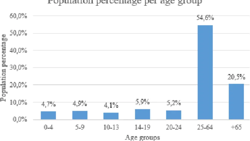
To contextualize and describe the population that lives in the same region as where the ED is located, the hospital is situated in a region that according to the Portuguese census of 2011 has a population density of 2478.8 per km2. Most of the population is aged between 25 and 64 years old (54%), while 20.5% has over 65 years old. Regarding unemployment, 14.33% of the population is unemployed (Fig. 3).

(29)

15

Fig 3 - Population age distribution according to the Portuguese 2011 Census

As previously mentioned, during the triage process, the patient is categorized in a triage colour according to the MTP. This protocol defines the recommended time limit for the patients to be taken care of, dividing them into five different possible triage colours: red, orange, yellow, green and blue. The possible triage colours and the respective recommended time limits are represented in Table 1.

Colour Treatment Recommended time limit (in minutes)

Red Immediate 0

Orange Very urgent 10

Yellow Urgent 60

Green Standard 120

Blue Non-urgent 240

Table 1 - Manchester Triage Protocol

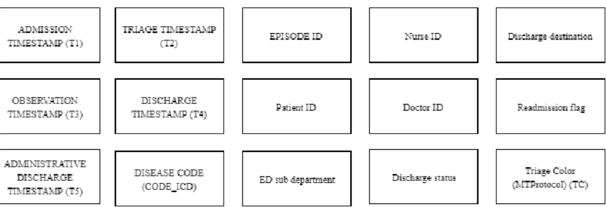
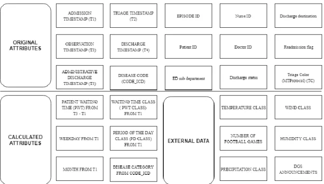
As stated before, there was a total of 15 attributes on the original dataset (Fig. 4). Five of those fifteen attributes correspond to a timestamp (in the dd-MM-YYYY hh:mm:ss format) for the steps above of the ED flow, so admission timestamp (T1), triage timestamp (T2), first observation timestamp (T3), discharge (T4) and administrative discharge (T5).

(30)

16 Another attribute on the dataset was the triage color (TC), that represented the triage color that was attributed to the patient when he went through the triage process. The possible values for this attribute are the colors defined in the MTP, stated in Table 1.

There was also information regarding the discharge, like the discharge status (a flag indicating if the discharge was attributed or not) and its respective discharge destination (for the cases where the patient was discharged). Another flag in the dataset was the readmission flag, indicating if the record represents an episode where the patient was readmitted or not.

There were also identifiers (id’s) to identify the doctors, nurses and patients involved in the event. Starting by the doctors, there were id’s for the doctors responsible for the patient first observation (third step on the ED flow) and discharge (fourth step in the ED flow). There was also an id to identify the nurse responsible for the patient triage (second step in the ED flow). Regarding the patient, there was the patient internal ID (to identify the patient and to track his history) and finally an identifier for the episode or event record. Since these aforementioned id’s were used to identify staff or patients, the data extraction was followed by an anonymization process, in order to be compliant with the European Union General Data Protection Regulation (GDPR) and to protect the patients and clinicians privacy, transforming the id’s to another number sequence to avoid the patient, ED staff or event identification. The hospital approach to privacy is that the health information can be used for research, but not for patient identification.

During the aforementioned anonymization process, the information that needs to be hidden (in this case, patient, doctor and nurse information) is encrypted. The correlation between the encrypted data and the original non-encrypted data can only be performed with a key (master key). This encryption and decryption process was based on a standard encryption process using both asymmetric-key algorithm like RSA (used to decrypt the symmetric key and consequently the data) and symmetric-key algorithm like AES (used to encrypt the data).

Finally, the last two attributes were the ED sub-department where the event took place and the patient ICD disease code for that occurrence. This last attribute, the patient ICD disease code (CODE_ICD) corresponds to the International Classification of Diseases (ICD9) code. These codes are managed by the World Health Organization (WHO) and allow to statistically classify and analyze diseases. Each disease has a code that is ordered according to disease similarity, which allows group diseases into bigger categories.

(31)

17 The mentioned attributes are summarized in Fig. 4

Fig 4 - Original dataset attributes list

3.2. Data Pre-Processing

This is the second process regarding the methodology used during this research. The main goal of this process is to prepare the data for the rest of the research.

Having faulty data can compromise the research results and analysis, meaning that it is important to ensure that the data is valid and veracious, respecting some of the big data characteristics [10]. To ensure that the data is valid and won’t compromise the results of the research, several data cleansing actions were taken in order to remove inconsistent data. The author considered as inconsistent, the records that have missing values or outlier values on any of the attributes.

To attempt to improve the results of the research, the author also added external data. The new added attributes were related to the weather conditions on the day of the patient visit to the ED, number of football games from the teams with the most supporters in Lisbon for that same day and finally if there was any official statement from the DGS (Direcção-Geral da Saúde) for that day. DGS is a Portuguese government health institution that has several intervention areas, being one of them to analyze and release public health information.

This process is described in more depth in Chapter 4.

3.3. Statistical analysis

After the data is cleaned and ready to be used for research, the author performed statistical analysis, to extract knowledge and gain more insights about the data being used

(32)

18 in the research. This knowledge discovery can be done through pattern identification in the data. The author considers the existence of a pattern when it is possible to describe a whole subset of data.

To perform this analysis, the author used Power BI tool from Microsoft and calculated maximum, minimum, average values of patient waiting time. Simple dashboards to analyze the distribution for some variables that were considered essential and were related with the average waiting times by the ED management were also created. An example for those variables are the average waiting times distribution per triage color, period of the day, weekday or month. The author also configured the schedule refresh option on Power BI, which will refresh the data that is fed to the dashboards automatically on a weekly basis.

These insights were valuable for the data mining process (last process of Figure 1). This process is described in more depth in Chapter 5.

3.4. Predictive Analytics through Data Mining Approach

Finally, in the last process, the data mining process, the author applied data mining techniques in order to discover hidden patterns in the data that was worked in the previous sections.

In this section, the author built a prototype that allows predicting the emergency department waiting time. This prediction was done using supervised learning techniques developed in R as a programming language. To validate the performance of the applied algorithm, the author used the “r-miner” library.

Then, the most important factors that affect the patient waiting time were also studied, to help the developed prototype users make the most informed decisions.

(33)

19

Chapter 4 – Data Pre-Processing

In this process, referenced as II – Data Pre-Processing in Fig.1, all the data collected the previous process, referenced as I – Data Collection in Fig.1, was analyzed and inconsistent data was removed (section 4.1 Inconsistent Data). Then, to improve the data, the author added external data attributes related to each day of the event. These new attributes were the weather conditions, the number of football games from the two teams with most fans in Lisbon and if there was an official statement from the DGS (Direção Geral de Saúde). DGS is a Portuguese governmental institution that has several goals, being one of them to manage public health information.

4.1. Inconsistent data

The main goal of this action was to remove inconsistent data. As aforementioned in the previous section, data needs to be valid and veracious to not compromise the results of the research. So, to ensure that the data was ready to be used in the research, several data cleansing operations were performed, allowing to remove inconsistent data. The author considered as inconsistent data any record that had missing values or outlier values on any of the attributes. Also, new attributes were calculated, based on the existing ones, in order to get more information from the available data. The calculation of these new attributes is explained below.

The author developed a script in Python 3.6, using the pandas and numpy python libraries to analyze and manipulate the data. The first operation of the script was to drop any data row (that represents an event) with null values on any of the attributes, using pandas drop.na() function. This resulted in the removal of 11 598 records, which represented almost 4% of the original dataset.

Then, the author calculated the patient waiting time, considering it as the time that the patient had to wait in order to be observed by a clinician. To calculate this, the author subtracted the timestamp from when the patient was admitted to the ED (admission timestamp), attribute identified with T1 in Fig. 4, from the timestamp of when the patient was first observed by a clinician (observation timestamp), attribute identified with T3 in Fig. 4. Before doing this, these timestamps had to be converted to python datetime objects, so that the subtraction could be performed and the calculated patient waiting time could also be stored as datetime object, which allowed future datetime manipulations like

(34)

20 converting the timestamp to seconds. After these calculations were finished, the author noticed that some of the waiting times were inconsistent since they were negative, which means that for that record, the observation timestamp (T3) was smaller than the admission timestamp (T1), something that is not possible to happen, since according to the hospital’s ED flow (reported in Fig. 1), the observation only happens after the patient admission. This resulted in the removal of 1 144 records, which corresponded to 0.4% of the original dataset. Still looking into the patient waiting time, the maximum value for the waiting time was 81 days. This showed that there were still inconsistent values as it was impossible for any patient to wait for 81 days to be observed by a doctor after being through the triage process in this ED. To correctly handle these high values, at first, the author attempted to use the 98 percentiles (includes only the records with the first 98% patient waiting times), but this would still leave records with 5 days of patient waiting time, which is still considered unrealistic by the ED management. On the other hand, if the author considered the 97 percentiles, the maximum waiting time was 5 hours. So, the author concluded that this would not be a good strategy to manage the outliers on this dataset and instead, considered as outliers, the records where the patient waiting time was higher than one day. This means that all the records where the patient waiting time was higher than a day were removed.

Other calculated attributes were the day of the week where the patient was admitted and the month of admission. Both of these attributes calculation was based on the admission timestamp (T1 in Fig. 4), using python’s weekday() and month() function respectively. These functions could only be applied because the timestamps were converted to python’s datetime objects before.

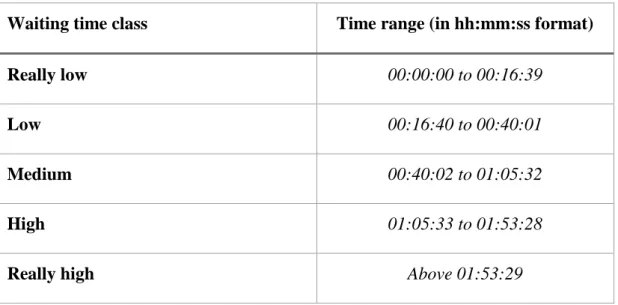
The previously calculated patient waiting time had continuous values. For example, 00:02:51 had no particular meaning, so in order to extract knowledge, these continuous values should be discretized in different classes, to improve the statistical analysis capability. The author discretized this variable (referenced as PWT in Fig. 5) into five different classes. The author chose five classes as a commitment between knowledge extraction and prediction efficiency, if there were fewer classes, the predictive power would increase, but there would be less knowledge to be extracted since the classes would have a bigger range. The python pandas qcut function was used to do this discretization. This function discretized the variable in equal sized classes (equal length bins), meaning

(35)

21 that all classes had the same ammount of events. The generated classes and the respective time ranges are explained on Table 2.

Waiting time class Time range (in hh:mm:ss format)

Really low 00:00:00 to 00:16:39

Low 00:16:40 to 00:40:01

Medium 00:40:02 to 01:05:32

High 01:05:33 to 01:53:28

Really high Above 01:53:29

Table 2 - Waiting time discretized classes

Another field that was calculated through discretization was the period of the day class, which corresponds to the period of the day where the patient was admitted, based on the admission timestamp (T1 from Fig. 4). The author also used the python pandas qcut function to discretize this attribute in five different classes. These possible values for each of these classes are explained in Table 3.

Period of the day class Time range (in hh:mm:ss format)

First class 00:00:00 to 09:41:57

Second class 09:41:58 to 12:27:11

Third class 12:27:12 to 15:34:53

Fourth class 15:34:54 to 19:07:57

Fifth class 19:07:58 to 23:59:59

Table 3 - Period of the day discretized classes

Other important atribute was the disease code (CODE_ICD from Fig. 4), that represents the ICD9 code associated with the disease that the patient suffered. As previously mentioned, each disease code is associated to a certain disease category. This is a way to discretize the disease codes, so the author calculated a new attribute called disease category, by matching the available disease code to the correspondent ICD9

(36)

22 disease category. To perform this operation, the author created a document with all the available ICD9 categories and their correspondent disease code ranges and used the pandas loc function to match the new attribute of disease category. This function allows to associate a value to a certain record, based on a boolean condition.

After this, the data was considered consistent and valid, so the author proceeded to the next step, where as aforementioned, external data was added.

4.2. External data

After preparing the hospital’s ED collected data, the author enriched it with external data, in order to improve the dataset and boost the predictive capability.

The first data to be added was associated with the weather information for the day of the event, based on the admission timestamp (T1 from Fig. 4). The author collected the weather information from 2015 January 1st_{to 2017 December 31}st_{, from the} wunderground service (www.wunderground.com). This service collects information hourly, from a single point in the city (weather station), in this case, near the Lisbon airport, also providing an average for each attribute for that day. The author collected the average values for each day on the aforementioned period, for the following attributes: temperature, humidity, wind and precipitation. Since these attributes were continuous, they were also discretized in five different classes, using the same process for discretization as mentioned before. The inclusion of these attributes in the dataset allowed the author to try to understand the weather influence on the patient waiting times.

Other external data that was collected were the number of football games, from the two main teams from Lisbon (Sporting CP and SL Benfica), from 2015 January 1st to 2017 December 31st. For each day during the aforementioned period, the number of games of any of the previously mentioned teams, was added up and stored in an attribute that represents the number of football games from those teams for that day. The data was collected from the zerozero platform (www.zerozero.pt), a website with a large football database, with the football, matches history, results, players, news, etc. Adding this information to the dataset allowed the author to try to understand the influence of football games on the ED demand and correspondent waiting times. During the research, the author held several meetings with the hospital’s ED management, and they considered

(37)

23 that it was expected for football games to be a big factor to influence the patient waiting times.

Finally, the last external data to be added to the studied dataset was the public health history from 2015 January 1st to 2017 December 31st. Using the “Direcção Geral de Saúde (DGS)” website, the author collected the main events (disease outbreaks, heat waves, vaccines shortage, etc.) that happened during the previously mentioned time period. This allowed the author to understand the influence of the DGS announcements on the patient waiting times, since some of those announcements could lead to more patient interactions with the health system.

To add all of this previously external data attributes to the original dataset, the author used the pandas merge function, that merges two datasets based on common keys, which in this case were the date of the event records (the admission date on the hospital data, reported as T1 in Fig. 4) and the date of the external events (the date of the weather conditions on the weather conditions dataset, the date of the game on the football games dataset and the date of the DGS public announcement on the public health history dataset). The structure of the dataset after the data pre-processing process is reported on Fig. 5 below.

Fig 5 - Attributes used during the research

After this process, there should be no faulty data, meaning that the dataset was ready for the next processes where the data were analyzed, and data mining techniques were applied, allowing to extract knowledge and make conclusions.

(38)

(39)

25

Chapter 5 – Statistical Analysis

In this process, represented as III – Statistical analysis in Fig.1, using the data collected and processed on the previous sections (whose attributes structure is exposed on Fig. 5), the author performs statistical analysis in order to find patterns and gain more insights. It is considered as finding a pattern when it is possible to describe a subset of data, being that description of the pattern. In this process, the author analyzed and studied some variables that are considered necessary by the ED management like the patient waiting times, attendance, disease distribution or fluctuation through the periods of the day, for example.

Starting with the average patient waiting time, it is 01:12:00 (in the hh:mm:ss format). Regarding the average patient waiting times per triage color, as expected, according to the MTP, the most urgent classes like red and orange have lower average waiting times, while the less urgent triage colors have higher average waiting times. The average waiting times per triage color are represented on the table 4 below.

Triage color Average waiting time (hh:mm:ss)

Red 00:19:20

Orange 00:35:18

Yellow 01:09:23

Green 01:26:05

Blue 02:02:12

Table 4 - Average waiting times per triage color

When looking into the average patient waiting time per month, the month of December has the longest average patient waiting time (01:24:21 in the hh:mm:ss format). The month with the lowest average patient waiting time is May (01:08:23 in the hh:mm:ss format).

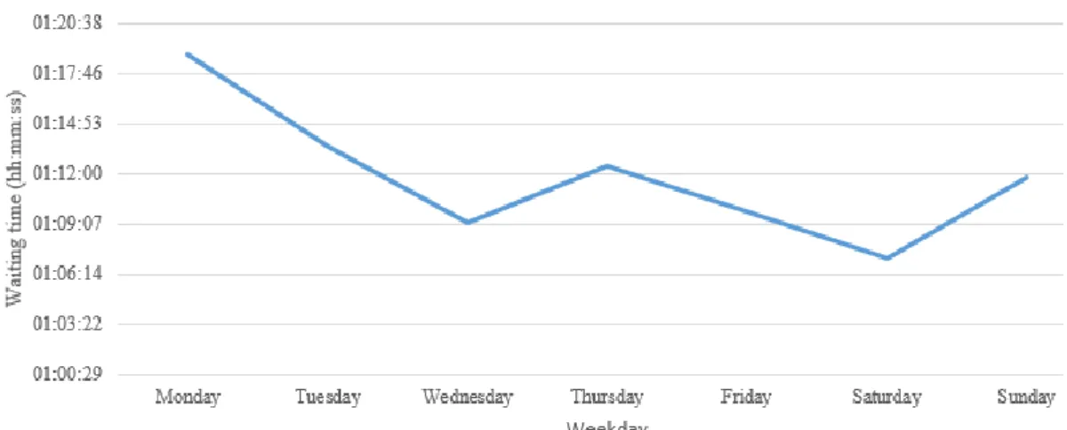
Making the same analysis but through the day of the week, Monday is the day with the longest average waiting time, 1:18:50 (hh:mm:ss). The average waiting time decreases throughout the week, except for Thursday (1:12:25 hh:mm:ss) and Sunday (1:11:44

(40)

26 hh:mm:ss) where there are small increases. The graph on Fig.6 represents the evolution of the average waiting time per day of the week.

Fig 6 - Average waiting time distribution through a day of the week

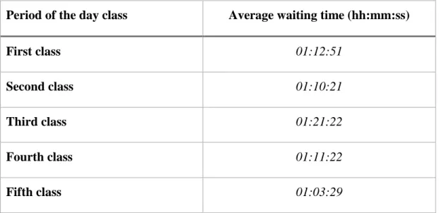
Regarding the patient average waiting time distribution through the period of the day, a variable that was discretized in the previous section and whose possible values are explained on Table 3, the period of the day with the lowest average waiting time is the last period, from 19:07:58 to 23:59:59, with an average patient waiting time of 01:03:29, in the hh:mm:ss format. On the other hand, the period with the highest average waiting time is the third class, that ranges from 12:27:12 to 15:34:53, with an average waiting time of 1:21:22 (hh:mm:ss format). The distribution of the average patient waiting time through the period of the day classes (available in Table 3) is available on Fig. 7 below.

Fig 7 - Average waiting time per period of the day

The average waiting time for each period of the day class is represented on the Table 5 below.

(41)

27

Period of the day class Average waiting time (hh:mm:ss)

First class 01:12:51

Second class 01:10:21

Third class 01:21:22

Fourth class 01:11:22

Fifth class 01:03:29

Table 5 - Average waiting time per period of the day class

Still regarding the period of the day classes, explained in Table 3, some classes have a longer range than others, even though this attribute was discretized using an equal areas method, where all classes have the same number of events. This happens because the attendance of the ED is not the same throughout the day. The period of the day classes with shorter range, like the second class (duration of 2 hours 45 minutes and 13 seconds) represent periods of higher attendance. On the other hand, longer classes like the first one (with a duration of 9 hours 41 minutes and 57 seconds) represent periods of less attendance, needing more time to reach the same number of occurrences as the other classes.

Regarding the triage color, most of the occurrences fall into the yellow or green triage categories, 40.9%, and 40.07% respectively. The triage color red, which according to the MTP represents the most urgent cases, covers only 0.73% of the occurrences. The number of event records per triage color is available in Fig. 8 below.

(42)

28

Fig 8 - Percentage of records per triage color

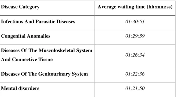
Regarding the disease categories, Table 6 below represents the top five disease categories with the longest average waiting time.

Disease Category Average waiting time (hh:mm:ss) Infectious And Parasitic Diseases 01:30:51

Congenital Anomalies 01:29:59

Diseases Of The Musculoskeletal System

And Connective Tissue 01:26:34

Diseases Of The Genitourinary System 01:22:36

Mental disorders 01:21:50

Table 6 - Top five disease categories with the longest average waiting time

Regarding the added external events, starting by the analysis the football games influence on the average waiting time, there is a minimal decrease on the average waiting time when there is one football game on that day. On the days where there are no football games, the average waiting time is 1:12:07 (hh:mm:ss). On the other hand, if there is one football game from the any of the two analyzed football teams on that day, the average waiting time is 1:11:13 (hh:mm:ss). If there are two games from those same teams on that day, the average waiting time is 1:12:44 (hh:mm:ss). These differences are so subtle that it was not possible for the author to conclude if there was an influence of the football games or not.

(43)

29 When looking at the other external data that was added, the announcements from the DGS, when there were announcements regarding the lack of vaccines for a specific disease, the average patient waiting time decreased, from 1:12:00 (average waiting time without any announcement in the hh:mm:ss format) to 1:03:46 (hh:mm:ss). On the other hand, the announcement of the outbreak of Legionare diseases in fall 2017, the average waiting time increased to 1:18:54 (hh:mm:ss). Other announcements like the increase of temperatures during the summer, the decrease of temperatures during the winter, pollution from wildfires or measles disease outbreak did not have any noticeable influence on the average waiting times.

The author also performed an analysis of the most common disease categories. Considering that there are in total 19 possible disease categories, there are two that stand out from the rest, which corresponds to “Symptoms, Signs and Ill-defined conditions” (18.76%) and “Injury and Poisoning” (18.29%). The third most common disease category is “Disease of the Musculoskeltal system and connective tissue” (8.76%).

Looking into the distribution of the disease categories throughout the year, the “Diseases of the respiratory system” decrease throughout the year, covering 10.2% of the events in January, 7.84% in March and 6.23% in June. In September, the number of “Diseases of the respiratory system” starts growing again (6.74%), reaching 11.12% in December. This was already expected, as the respiratory diseases are seasonal, having more prevalence during the Winter season and less in the Summer. The monthly distribution of the “Diseases of the respiratory system” is reported in Fig. 9.

Fig 9 - Monthly distribution of "Diseases of the respiratory system."

(44)

(45)

31

Chapter 6 – Predictive Analytics through Data Mining Approach

This is the fourth process described on Fig.1, represented as IV – Data Mining, where the author built a prototype to predict the patient ED waiting time. Data Mining techniques were applied to find hidden patterns and study the most efficient ways to improve ED patient waiting time. The prototype was built using R programming language with R studio. This approach was complex due to the number of attributes in the dataset, 28, as reported in Fig. 5.

This prototype consists of a system which is described in Fig. 10 and is based on three phases. The first phase corresponds to the phase where the user introduces inputs, which can be any of the variables used to train the predictor model (section 2), represented in Fig. 11. Then, those inputs are fed to a predictor model (section 2 on Fig. 10) based on an algorithm. The author applied the algorithms in three different scenarios, each one of them using different variables as input, in order to try and find the most accurate one. Finally, this model will compute an estimation for the patient waiting time, based on the conditions that were inserted on the first phase by the user. Since the user can not insert some attributes because they are only attributed while at the hospital after the triage process, like the triage color or the disease category, it is produced an estimation per possible value for any of those attributes. Summarizing, it is produced an estimation for all possible values of triage color and disease category.

Fig 10 - Prototype schema

6.1 – Predictor Model description

The second section of the prototype is based on a trained model of an algorithm. The author tested two algorithms and optimized the model by experimenting several input formulas, creating different scenarios, until reaching the one with the most accuracy.

The researcher applied both Naïve Bayes (NB) and Random Forest (RF) algorithms. Starting by the NB, it is a probabilistic classifier, that considers each variable as independent and then associates it to a conditional probability. This conditional

(46)

32 probability is calculated based on the Bayes theorem and can be expressed on the following equation:

𝑃(𝐶|𝐴) = 𝑃(𝐴|𝐶)∗ 𝑃(𝐶)

𝑃(𝐴) (1)

Looking into the equation (1), it shows that the algorithm calculates the probability of an event, based on something that already occurred. In this case, C corresponds to the probability for any of the possible waiting time classes, while the A corresponds to the conditions known and used as input to discover the waiting time class, which can be for example the weather conditions, a period of the day, the day of the week, month, etc.

Another algorithm that the author applied was the RF algorithm. The author chose to apply this algorithm because it was applied by [31] on waiting time prediction where it was concluded that it performs more accurate predictions than other regression models.

This algorithm builds several decision trees using bootstrap samples from the training dataset, randomly choosing predictor variables for every node. Then, in a process called bagging, it calculates the mean or majority class from all of those samples, producing the final output. This helps to avoid overfit and increases the accuracy of the model [31] , by creating small subsets of trees, while the decision tree algorithm has a unique decision tree, meaning that it will be deeper and denser, a possible cause for overfitting.

Summarizing, for all of the trees given as input for the algorithm, it will produce a bootstrap sample from the training dataset. Then, it will build a tree by randomly selecting a subset of variables and for every node of that tree and based on the values of those chosen variables it will generate new nodes until it reaches a defined minimum node size. Finally, it will produce a prediction, by averaging the result of all those produced trees.

As stated before, the NB algorithm calculates the conditional probability for all possible values of the predictor variable. If there are too many possible values for the predictor variable, then it would have a bad performance. A similar logic applies for the RF algorithm since if it has more possible values, the generated trees will be larger. For this reason, it is essential to discretize the continuous data before applying the algorithms, creating classes for that variable. The author already discretized the patient waiting time and the period of the day attribute in section II – Data Pre-processing (Chapter 4). The possible values for each variable are in Table 2 and Table 3, respectively.

(47)

33 Since some attributes were not crucial for the prediction or they were already represented through another attribute, they were removed.

Summarizing, the variables used as input for this phase were: triage color, the day of the week, month, a period of the day, disease category, number of football games, DGS announcements, temperature class, wind class, humidity class, sea level class and precipitation class. The rest of the attributes were removed from this dataset.

The variables of this new dataset that was used to apply the algorithms are exposed to Fig. 11. The names between the parenthesis represent the abbreviation for each variable, which can be used on the rest of this section.

Fig 11 - Variables used in the dataset to apply the algorithms

(48)

34

Attribute Possible values

Waiting time class Really low (00:00:00 to 00:16:39); Low (00:16:40 to 00:40:01); Medium (00:40:02 to 01:05:32); High

(01:05:33 to 01:53:28); Really high (above 01:53:29)

Triage color Red; Orange; Yellow; Green; Blue

Weekday Monday; Tuesday; Wednesday; Thursday; Friday; Saturday; Sunday

Month January; February; March; April; May; June; July; August; September; October; November; December

Disease Category Infectious And Parasitic Diseases; Neoplasms; Endocrine, Nutritional And Metabolic Diseases; And

Immunity Disorders; Diseases Of The Blood And Blood-Forming Organs; Mental disorders; Diseases Of The Nervous System And Sense Organs; Diseases Of The Circulatory System; Diseases Of The Respiratory System; Diseases Of The Digestive System; Diseases Of The Genitourinary System; Complications Of Pregnancy, Childbirth, And The Puerperium; Diseases Of The Skin And Subcutaneous Tissue; Diseases Of The Musculoskeletal System And Connective Tissue; Congenital Anomalies; Certain Conditions Originating In The Perinatal Period; Symptoms, Signs, And Ill-Defined Conditions; Injury And Poisoning; Supplementary Classification Of Factors Influencing Health Status And Contact With Health Services; Supplementary Classification Of External Causes Of Injury And Poisoning

Period of the day First class (00:00:00 to 09:41:57); Second class (09:41:58 to 12:27:11); Third class (12:27:12 to 15:34:53);

Fourth class (15:34:54 to 19:07:57); Fifth class (19:07:58 to 23:59:59)

Number of football games

0; 1; 2

DGS Announcements Measles outbreak; Lack of vaccines; Pollution from wildfires; Legionnaire disease outbreak in Lisbon;