Carlos Pestana Barros & Nicolas Peypoch
A Comparative Analysis of Productivity Change in Italian and Portuguese Airports
WP 006/2007/DE _________________________________________________________
Maria Cândida Ferreira
Financial Integration in European Countries: Some Panel
Evidence
WP 21/2010/DE/UECE _________________________________________________________
Department of Economics
W
ORKINGP
APERSISSN Nº 0874-4548
Financial Integration in European Countries: Some Panel Evidence
Cândida Ferreira [1]
Abstract
This paper provides empirical evidence of the financial integration of some developed countries, mostly in the European Union, covering the period between 1961 and 2008.
The main contributions are to be found first, in the application of panel estimates and test statistics. particularly of some recently developed tests like the Westerlund (2007) bootstrap cointegration tests and the Pesaran (2004) test of cross-sectional independence, using the available AMECO series of nominal and real long-term and short-term interest rates as well as the yield curve; secondly, in the comparison of the approximations between the countries’ series of rates and those of two chosen benchmarks: the German and US rates, for six panels of EU and some non-EU countries during three specific time intervals.
The obtained results allow us to draw conclusions not only on the quite high degree of approximation towards the benchmark rates, particularly those of Germany, but also on the differences in the patterns of this approximation before and after the implementation of the Single Market Program and of the EMU. Furthermore, we draw conclusions on some specific characteristics of the considered series of rates and, in particular, of the yield curves.
Keywords: Financial integration; European integration; panel estimates; cointegration tests.
JEL Classification: C33; E43; E44; F36.
[1]
ISEG-UTL - Instituto Superior de Economia e Gestão – Technical University of Lisbon and UECE – Research Unit on Complexity and Economics
Rua Miguel Lupi, 20, 1249-078 - LISBOA, PORTUGAL tel: +351 21 392 58 00
2
Financial Integration in European Countries: Some Panel Evidence
1. Introduction
Since the 1970s, and particularly after the collapse of the Bretton Woods system, followed by the
first acute, deep oil crisis, there has been a global trend to reduce the barriers to free international
trade, to increase direct foreign investment and also to establish a clear process of international
financial liberalisation (Dooley, 1996; Obstfeld, 1998; Maggi, 1999; Mansfield et. al. 2000, Rose
and Wincoop, 2001; Baier and Bergstrand, 2007).
In Europe, over the past half-century, a remarkable process of integration has taken place with the
aim of guaranteeing the stability and security of the continent. This process started with the
common undertaking of six countries to create the European Coal and Steel Community in 1951,
the forerunner of the European Economic Community (EEC) which was established in 1958. By
2007, the EEC had evolved into the European Union (EU), incorporating 27 member-states.
At the same time, and at least since the 1960s, there were proposals for a single currency as a way
to enhance the process of integration of the member-states. However, it was only in the 1992 that
the Maastricht Treaty led to the creation of the single European currency - the euro - and the
European Monetary Union (EMU).
The establishment, first, of the Single Market Program and then, of the EMU was supposed to
accelerate the process of consolidation and economic and financial integration not only between
the countries in the euro area but also in the European Union as a whole. The process of financial
integration is also quite often presented as a necessary pre-requisite for the adoption of the euro
and the implementation of the single monetary policy, with the predominance of the banking
intermediation in the context of the EU (Cabral et al., 2002; European Central Bank, 2003;
Hartman et al., 2003; Baele et al., 2004; Sørensen and Gutiérrez, 2006).
However, there is no clear consensus on the evidence of increasing consolidation and integration
of the European markets and some empirical studies have even concluded that the European
financial markets are far from being integrated (Monti, 1996; Gardener et al., 2002, Affinito and
Farabullini, 2006; European Central Bank, 2007; European Central Bank, 2008; Gropp and
Kashyap, 2008).
One of the explanations for the lack of consensus is to be found in the fact that financial
3 process is theoretically linked to the law of one price and the notion that “financial integration in
euro area financial markets is achieved when all economic agents ... face identical rules and have
equal access to financial instruments or services in those markets” (Baele et al. 2004, pp. 5).
This definition has direct and important implications for the methodologies and measures that are
usually adopted in the degree of integration across the different market segments. The analysis
uses a set of quantitative indicators of financial integration which require available and fully
compatible series of data. So the empirical studies face a particular dilemma: either to use longer
series for a small number of countries, or to use sets including more countries, but for only
relatively short time periods.
This paper endeavours to overcome the above-mentioned dilemma by using the available AMECO
series of nominal and real long-term and short-term interest rates, as well as the yield curves. It
contributes to the empirical research into the degree of financial integration across different sets of
EU and some non-EU countries and the time period between 1961 and 2008.
The main questions to be answered are:
1) In a world of international financial liberalisation, is there a clear process of
European integration and is it more relevant than the global process of integration? In
attempting to answer this question, we not only always include some non-European
countries in our panels, but also choose two particular benchmarks: the German and US
rates.
2) Is it possible to identify different patterns of approximation towards the
benchmark rates for different panels of more or less homogeneous countries over
particular time intervals? Our panels begin with only 9 EU countries and end with 25
EU countries, taking into account the possible influences of the implementation of the
Single Market Program after 1985 and the inception of the EMU in 1999.
3) Are there any differences in the patterns of approximation towards the
benchmarks of the nominal, real long-term or short-term interest rates, or of the yield
curves? Here, we use all available AMECO interest rate and yield curve series,
differentiating not only the short-term from the long-term rates, but also the nominal
4 The remainder of this paper is structured as follows. The next section presents the methodological
framework and the data. Section 3 reports the obtained results with “first” and “second” generation
panel unit root and cointegration tests. The cross-sectional independence test, which was applied
after panel fixed-effects estimates, is presented in Section 4. Section 5 reports the obtained results
with three-stage panel estimations. Section 6 concludes.
2. Methodological Framework and Data
From the existing literature on measuring financial integration, we mainly follow the important
contributions of Adam et al. (2002), Adjaouté and Danthine (2003) and Baele et al. (2004). These
authors present several price-based and quantity-based indicators and models which may be
adapted to the empirical measure of financial integration through yield differences in individual
countries or markets.
Taking into account that, theoretically, in a perfectly integrated market we would have an ideal
yield, one of the proposed measures could be the comparison between a particular (country, market
or segment) yield and the ideal one. Since the ideal yield is not observable, Adam et al (2002) and
Adjaouté and Danthine (2003) propose a second-best alternative, using a determined benchmark
yield as a proxy for the ideal one.
Another method that is widely used in this type of study (among others by Adam et al., 2002;
Hartmann et al., 2003; Baele et al., 2004 Sander and Kleimeier, 2004; Vajanne, 2007; European
Central Bank, 2007 and 2008) adapt the beta, and sometime also the sigma, convergence models
that are borrowed from the literature on economic growth.
In the present paper, we will adapt these models and as we aim to compare the degree of
integration among EU countries and some non-EU countries, we will always consider two possible
benchmarks: the German and US yields or interest rates.
We apply the following general regression model to our panels with n series, for i countries and t
time periods:
Rn = αn + βn ∆nb + εn [ 1]
Where, for all n series we have:
αn = intercept
5 ∆nb = the differences between each country’s rate and one of the benchmark’s rate.
εn = error term
The use of the available AMECO series is a guarantee for the compatibility of all data. We select
the series of nominal and real (both by private consumption and the GDP deflators) long-term and
short-term interest rates, as well as the yield curves. They allow us to compare the evolution of the
degree of integration between some EU and a few, but relevant, non-EU countries in different time
periods.
We will consider six panels of countries in three time intervals:
1) A panel with 432 observations for 48 years (1961-2008) and 9 EU countries (Belgium, Denmark, Finland, France, Germany, Italy, Netherlands, Sweden and the United Kingdom);
2) A panel with 480 observations for the same 48 years (1961-2008) and 10 countries (the above EU-9 plus the USA);
3) A panel with 336 observations for 24 years (1985-2008) and 14 EU countries (Austria, Belgium, Denmark, Finland, France, Germany, Greece, Ireland, Italy, Netherlands, Portugal, Spain, Sweden, the United Kingdom);
4) A panel with 408 observations for the same 24 years (1985-2008) and 17 countries (the previous EU-14 plus Japan, Norway and the USA);
5) A panel with 250 observations for 10 years (1999-2008) and 25 EU countries (all the actual EU members except Luxembourg and Romania);
6) A panel with 290 observations for the same 10 years (1999-2008) and 29 countries (the same EU-25 plus Japan, Norway, Switzerland and the USA).
Taking into account our aim to compare the degree of integration among EU countries and some
non-EU countries, we choose two benchmark countries: Germany and the USA; we use the
provided series to calculate, for each of the selected countries, the differences between the
country’s rate and Germany’s rate, as well as the difference between the country’s rate and the US
rate1.
1
6 So, for each of the six panels, we will consider the following variables:
1. ILN = Nominal long-term interest rates
2. ILRC = Real long-term interest rates, deflator private consumption 3. ILRV = Real long-term interest rates, deflator GDP
4. ISN = Nominal short-term interest rates
5. ISRC = Real short-term interest rates, deflator private consumption 6. ISRV = Real short-term interest rates, deflator GDP
7. IYN = Yield curve
8. ∆ILN Germany = (ILN)i – (ILN)Germany
9. ∆ILRC Germany = (ILRC)i – (ILRC)Germany
10.∆ILRV Germany = (ILRV)i – (ILRV)Germany
11.∆ISN Germany = (ISN)i – (ISN)Germany
12.∆ISRC Germany = (ISRC)i – (ISRC)Germany
13.∆ISRV Germany = (ISRV)i – (ISRV)Germany
14.∆IYN Germany = (IYN)i – (IYN)Germany
15.∆ILN USA= (ILN)i – (ILN)USA
16.∆ILRC USA= (ILRC)i – (ILRC) USA
17.∆ILRV USA= (ILRV)i – (ILRV) USA
18.∆ISN USA= (ISN)i – (ISN) USA
19.∆ISRC USA= (ISRC)i – (ISRC) USA
20.∆ISRV USA= (ISRV)i – (ISRV) USA
21.∆IYN USA= (IYN)i – (IYN) USA
3. Panel Unit Root and Cointegration Tests
In the last few years, the literature and empirical estimations on panel unit root and cointegration
tests has advanced considerably and has begun to distinguish between the “first” generation tests,
which are mainly based on the assumption of cross-sectional independence among the panel units,
except for the common time effects, and the “second” generation tests which includes tests
allowing for different types of cross-sectional dependence among the panel units and tests allowing
for structural breaks.
Among the available “first” generation panel unit root tests, we choose to use the Levin, Lin and
Chu (2002) test and the Im, Pesaran and Shin (2003) test.
The Levin, Lin and Chu (2002) may be viewed as a pooled Dickey-Fuller test, or as an augmented
Dickey-Fuller test, when lags are included and the null hypothesis is the existence of
7 this paper, with fixed-effects and it assumes that there is a common unit root process. The results
reported in Appendix I allow us to reject the existence of the null hypothesis.
The Im, Pesaran and Shin (2003) test estimates the t-test for unit roots in heterogeneous panels and
allows for individual unit root processes. It is based on the mean of the individual Dickey-Fuller
t-statistics of each unit in the panel and assumes that all series are non-stationary under the null
hypothesis. Appendix II presents the obtained results and they confirm the rejection of the
non-stationarity.
Representing the “second” generation of tests, we implement four panel cointegration tests
developed by Westerlund (2007) and Westerlund and Edgerton (2007), which test for the absence
of cointegration by determining whether the individual panel members are error correcting. These
tests are very flexible2, working well in unbalanced, heterogeneous and/or relatively small panels
and they allow for dependence both between and within the cross-panel units.
These tests provide four test statistics: Gt, Ga, Pt and Pa. The Gt and Ga statistics test H0: ai = 0
for all i versus H1: ai < 0 for at least one of the series, i, starting from a weighted average of the
individually estimated coefficients ai and their respective t-ratios. The Pt and Pa test statistics
consider the pooled information of all panel cross-section units to test H0: ai = 0 for all i versus
H1: ai < 0 for all cross-section units. Thus, the rejection of the H0 has always to be taken as the
rejection of the cointegration for the whole panel. Any single cross-unit can cause the rejection of
the H0 and it is not possible to identify which cross-unit is responsible for this rejection.
In this paper, we apply the bootstrap version of the Westerlund (2007) cointegration test to the
seven rates included in our panel and their respective differences to the considered benchmarks:
the German and the US rates. For each of the considered panels of countries and time periods, we
report the obtained robust p-values3.
2
The application of these panel cointegration tests to the i series included in one panel will consider, for each moment t (during the time interval t=0,…,p), the following error-correction model:
Dyit = ci +ai1*Dyit-1 +…+ aip*Dyit-p + bi0*Dxit + bi1*xit-1 + …+ bip * Dxit-p + ai (yit-1 – bi*xit-1)+ uit
3
8
Table 1 - Bootstrap robust p-values obtained with the Westerlund (2007) panel cointegration test -
1961-2008
Cointegration
between the variables * EU9** EU9+USA Gt Ga Pt Pa Gt Ga Pt Pa
ILN and ∆ILNGermany 0.480 0.350 0.360 0.240 0.490 0.320 0.390 0.220
ILRC and ∆ ILRCGermany 0.020 0.000 0.000 0.000 0.010 0.000 0.000 0.000
ILRV and ∆ ILRVGermany 0.000 0.000 0.000 0.000 0.000 0.020 0.000 0.000
ISN and ∆ ISNGermany 0.030 0.040 0.020 0.020 0.030 0.040 0.010 0.000
ISRC and ∆ ISRCGermany 0.000 0.000 0.000 0.000 0.000 0.000 0.000 0.000
ISRV and ∆ ISRVGermany 0.000 0.000 0.000 0.000 0.000 0.000 0.000 0.000
IYN and ∆ IYNGermany 0.000 0.000 0.000 0.000 0.000 0.000 0.000 0.000
ILN and ∆ILNUSA 0.500 0.540 0.380 0.410 0.460 0.520 0.430 0.460
ILRC and ∆ ILRCUSA 0.340 0.300 0.320 0.270 0.280 0.200 0.200 0.150
ILRV and ∆ ILRVUSA 0.420 0.450 0.400 0.430 0.320 0.320 0.390 0.350
ISN and ∆ ISNUSA 0.220 0.260 0.140 0.160 0.160 0.160 0.070 0.080
ISRC and ∆ ISRCUSA 0.120 0.120 0.090 0.050 0.080 0.110 0.060 0.070
ISRVand ∆ ISRVUSA 0.160 0.220 0.060 0.060 0.120 0.110 0.070 0.050
IYN and ∆ IYNUSA 0.000 0.000 0.000 0.000 0.000 0.000 0.000 0.000
*
ILN = Nominal long-term interest rates; ILRC = Real long-term interest rates, deflator private consumption; ILRV = Real long-term interest rates, deflator GDP; ISN = Nominal short-term interest rates; ISRC = Real short-term interest rates, deflator private consumption; ISRV = Real short-term interest rates, deflator GDP; IYN = Yield curve; ∆ILN Germany = (ILN)i – (ILN)Germany; ∆ILRC Germany = (ILRC)i – (ILRC)Germany; ∆ILRV Germany = (ILRV)i – (ILRV)Germany; ∆ISN Germany = (ISN)i – (ISN)Germany; ∆ISRC Germany = (ISRC)i – (ISRC)Germany; ∆ISRV Germany = (ISRV)i – (ISRV)Germany; ∆IYN Germany = (IYN)i – (IYN)Germany; ∆ILN USA= (ILN)i – (ILN)USA; ∆ILRC USA= (ILRC)i – (ILRC) USA; ∆ILRV USA= (ILRV)i – (ILRV) USA; ∆ISN USA= (ISN)i – (ISN) USA; ∆ISRC USA= (ISRC)i – (ISRC) USA; ∆ISRV USA= (ISRV)i – (ISRV) USA ; ∆IYN USA= (IYN)i – (IYN) USA.
**EU9 = Belgium, Denmark, Finland, France, Germany, Italy, Netherlands, Sweden, United Kingdom
According to the results reported in Table 1, we can conclude that the differences between the left
and the right sides of the table are not relevant, meaning that the inclusion of the USA in the panel
of EU-9 countries does not provide any significant changes in the approximation between the
considered countries.
Reading across the lines of this table, we clearly see the differences between its first part, where
almost all p-values indicate strong approximation, both between and within the cross-units and in
the panel as a whole, demonstrating the approximation of the different countries’ interest rates to
the German patterns. The only exception is the series of the nominal long-term interest rate, which
reveals the individual behaviour of the included countries and is clearly not closed to the
differences to the German nominal long-term rate.
On the other hand, the lines of the second part of Table 1 evidently show that there is no
approximation with the USA´s patterns. The only exception is the series of the yield curves,
9
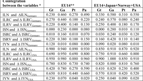
Table 2 - Bootstrap robust p-values obtained with the Westerlund (2007) panel cointegration test -
1985-2008
Cointegration
between the variables * EU14** EU14+Japan+Norway+USA Gt Ga Pt Pa Gt Ga Pt Pa
ILN and ∆ILNGermany 0.230 0.460 0.270 0.490 0.330 0.580 0.310 0.550
ILRC and ∆ ILRCGermany 0.270 0.440 0.100 0.220 0.240 0.570 0.080 0.240
ILRV and ∆ ILRVGermany 0.220 0.400 0.140 0.130 0.250 0.400 0.180 0.170
ISNand ∆ ISNGermany 0.000 0.230 0.000 0.080 0.000 0.280 0.010 0.110
ISRC and ∆ ISRCGermany 0.010 0.160 0.010 0.070 0.030 0.240 0.030 0.120
ISRV and ∆ ISRVGermany 0.220 0.380 0.100 0.150 0.160 0.420 0.110 0.140
IYN and ∆ IYNGermany 0.120 0.010 0.080 0.000 0.090 0.020 0.080 0.010
ILN and ∆ILNUSA 0.900 0.940 0.890 0.930 0.850 0.910 0.870 0.920
ILRC and ∆ ILRCUSA 0.690 0.950 0.690 0.800 0.750 0.910 0.660 0.800
ILRV and ∆ ILRVUSA 0.950 0.980 0.880 0.960 0.900 1.000 0.850 0.910
ISNand ∆ ISNUSA 0.780 0.830 0.730 0.740 0.820 0.880 0.810 0.760
ISRC and ∆ ISRCUSA 0.420 0.780 0.270 0.590 0.410 0.820 0.230 0.400
ISRV and ∆ ISRVUSA 0.650 0.810 0.440 0.660 0.570 0.810 0.420 0.520
IYN and ∆ IYNUSA 0.230 0.070 0.040 0.020 0.250 0.040 0.090 0.020
*
ILN = Nominal long-term interest rates; ILRC = Real long-term interest rates, deflator private consumption; ILRV = Real long-term interest rates, deflator GDP; ISN = Nominal short-term interest rates; ISRC = Real short-term interest rates, deflator private consumption; ISRV = Real short-term interest rates, deflator GDP; IYN = Yield curve; ∆ILN Germany = (ILN)i – (ILN)Germany; ∆ILRC Germany = (ILRC)i – (ILRC)Germany; ∆ILRV Germany = (ILRV)i – (ILRV)Germany; ∆ISN Germany = (ISN)i – (ISN)Germany; ∆ISRC Germany = (ISRC)i – (ISRC)Germany; ∆ISRV Germany = (ISRV)i – (ISRV)Germany; ∆IYN Germany = (IYN)i – (IYN)Germany; ∆ILN USA= (ILN)i – (ILN)USA; ∆ILRC USA= (ILRC)i – (ILRC) USA; ∆ILRV USA= (ILRV)i – (ILRV) USA; ∆ISN USA= (ISN)i – (ISN) USA; ∆ISRC USA= (ISRC)i – (ISRC) USA; ∆ISRV USA= (ISRV)i – (ISRV) USA ; ∆IYN USA= (IYN)i – (IYN) USA.
**EU14 = Austria, Belgium, Denmark, Finland, France, Germany, Greece, Ireland, Italy, Netherlands, Portugal, Spain, Sweden, United Kingdom.
Table 2 presents the bootstrap robust p-values obtained for the two panels during the time period
1985-2008, that is, after the implementation of the Single Market Program and the beginning of the
relevant EU enlargement processes. The 14 EU countries included in our panels are more
heterogeneous, as are the non-EU countries that we consider in the right column of the table, and
the results reveal their individualities. The differences between the two groups of countries are
now more evident and they indicate the greater heterogeneity of the panel when 3 non-EU
countries were added.
Generally speaking, and with very few exceptions, there are no clear cointegration relationships in
either panel. However, reading carefully across the lines, we still find some differences between
the first and the second parts of the table, revealing that the approximation to the German patterns
10 The few exceptions of approximation in the series behaviour are to be found in the short-time
nominal interest rate and, to a lesser extent, also in the real short-term interest rate (using the
private consumption deflator) which approximate to the German rates. This may be understood as
a symptom of the required monetary integration in the context of the EMU implementation
process. The yield curves also reveal their particular behaviour and are still much more correlated
than the other series.
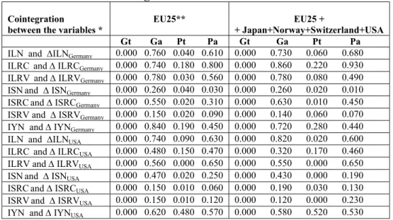
Table 3 - Bootstrap robust p-values obtained with the Westerlund (2007) panel cointegration test -
1999-2008
Cointegration between the variables *
EU25** EU25 +
+ Japan+Norway+Switzerland+USA Gt Ga Pt Pa Gt Ga Pt Pa
ILN and ∆ILNGermany 0.000 0.760 0.040 0.610 0.000 0.730 0.060 0.680
ILRC and ∆ ILRCGermany 0.000 0.740 0.180 0.800 0.000 0.860 0.220 0.930
ILRV and ∆ ILRVGermany 0.000 0.780 0.030 0.560 0.000 0.780 0.080 0.490
ISNand ∆ ISNGermany 0.000 0.260 0.040 0.030 0.000 0.260 0.020 0.010
ISRCand ∆ ISRCGermany 0.000 0.550 0.020 0.310 0.000 0.630 0.010 0.450
ISRV and ∆ ISRVGermany 0.000 0.150 0.020 0.090 0.000 0.140 0.060 0.070
IYN and ∆ IYNGermany 0.000 0.840 0.190 0.450 0.000 0.720 0.280 0.440
ILN and ∆ILNUSA 0.000 0.740 0.090 0.630 0.000 0.820 0.020 0.600
ILRC and ∆ ILRCUSA 0.000 0.480 0.150 0.470 0.000 0.320 0.170 0.460
ILRV and ∆ ILRVUSA 0.000 0.560 0.000 0.650 0.000 0.550 0.000 0.650
ISNand ∆ ISNUSA 0.000 0.470 0.020 0.250 0.000 0.430 0.000 0.190
ISRCand ∆ ISRCUSA 0.000 0.150 0.010 0.060 0.000 0.190 0.030 0.130
ISRVand ∆ ISRVUSA 0.000 0.150 0.010 0.120 0.000 0.120 0.000 0.230
IYN and ∆ IYNUSA 0.000 0.620 0.480 0.570 0.000 0.580 0.520 0.530
*
ILN = Nominal long-term interest rates; ILRC = Real long-term interest rates, deflator private consumption; ILRV = Real long-term interest rates, deflator GDP; ISN = Nominal short-term interest rates; ISRC = Real short-term interest rates, deflator private consumption; ISRV = Real short-term interest rates, deflator GDP; IYN = Yield curve; ∆ILN Germany = (ILN)i – (ILN)Germany; ∆ILRC Germany = (ILRC)i – (ILRC)Germany; ∆ILRV Germany = (ILRV)i – (ILRV)Germany; ∆ISN Germany = (ISN)i – (ISN)Germany; ∆ISRC Germany = (ISRC)i – (ISRC)Germany; ∆ISRV Germany = (ISRV)i – (ISRV)Germany; ∆IYN Germany = (IYN)i – (IYN)Germany; ∆ILN USA= (ILN)i – (ILN)USA; ∆ILRC USA= (ILRC)i – (ILRC) USA; ∆ILRV USA= (ILRV)i – (ILRV) USA; ∆ISN USA= (ISN)i – (ISN) USA; ∆ISRC USA= (ISRC)i – (ISRC) USA; ∆ISRV USA= (ISRV)i – (ISRV) USA ; ∆IYN USA= (IYN)i – (IYN) USA.
**EU-25 = all the actual EU members except Luxembourg and Romania.
The robust p-values obtained for the last two panels (one with EU-25 countries and the other with
4 non-EU countries included, both for the time period 1999-2008) are reported in Table 3 and they
clearly show the differences among the four test statistics provided by the Westerlund (2007) panel
cointegration tests.
Now for both panels, the Gt columns indicate clear integration between the countries’ rates,
revealing the importance of the approximation of the rates, for at least some countries in the
11 However, as expected in a dynamic world and with panels of quite heterogeneous countries, the Ga
and Pa p-values clearly point to non-integration, not only within at least one country, but also
overall for the pooled information of both panels.
4. Fixed-effects estimates and cross-sectional independence
In order to continue our analysis of the degree of integration between the considered countries’
rates and the two chosen benchmarks, we will apply panel fixed-effects estimates to the general
regression model represented by equation [1]
After each regression, we test the hypothesis of cross-sectional independence using the test
proposed in Pesaran (2004), which follows a standard normal distribution and is able to deal with
balanced and unbalanced panels. Here, we present not only the Pesaran statistic, but also the
average value of the off-diagonal elements of the cross-sectional correlation matrix of residuals.
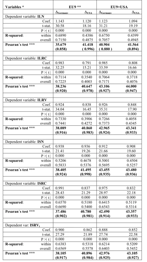
Table 4 reports, for our first two panels of countries (EU-9 and EU-9 plus USA, both for the time
period 1961-2008), the fixed-effects coefficients, t-statistics, p-values, the respective between and
overall R-squared values, as well as the Pesaran test results for all considered nominal and real
interest rates and the yield curves4.
The presented results confirm the better approximation of almost all considered rates to the
German rates than to the US rates. In addition, since the reported overall R-squared values are
always a little higher than the within R-squares, they also allow us to conclude that the
approximation is mainly between the different countries, our cross-units, for the same time
periods, rather than the approximation within each individual country during this relatively long
time interval.
The reported Pesaran results are in line with the previous conclusions.
They are always higher, revealing more independent relationships, when the explaining variable is
the difference between the country’s rate and the US rate.
Moreover, they confirm that in these two panels, the highest degree of integration is among the
yield curves, which, nevertheless, also reveal their specific characteristics. Now it becomes very
clear that the yield does not depend mostly on the approximation to the German patterns, rather
4
12 they reflect the dynamic character of the international financial markets, in which the USA still has
a dominant role.
Table 4 – Fixed-effects panel estimates and Pesaran (2004) test of cross-sectional independence -
1961-2008
Variables * EU9 ** EU9+USA ∆Germany ∆USA ∆Germany ∆USA Dependent variable: ILN
Coef. 1.143 1.120 1.123 1.094 t-stat. 30.58 18.16 31.21 19.19 P >| t | 0.000 0.000 0.000 0.000
R-squared: within overall
0.6890 0.4386 0.7150 0.4875
0.6750 0.4399 0.7057 0.4945
Pesaran´s test *** 35.679 41.418 (0.858) ( 0.996)
40.904 41.564 ( 0.880 ) (0.894)
Dependent variable: ILRC
Coef. 0.983 0.791 0.985 0.808 t-stat. 32.25 15.21 33.59 16.66 P >| t | 0.000 0.000 0.000 0.000
R-squared: within overall
0.7114 0.3540 0.7225 0.4003
0.7064 0.3718 0.7171 0.4076
Pesaran´s test *** 38.236 40.647 (0.920) (0.978)
43.106 44.000 (0.927) (0.947)
Dependent variable: ILRV
Coef. 0.924 0.838 0.926 0.848 t-stat. 34.04 16.45 35.31 17.90 P >| t | 0.000 0.000 0.000 0.000
R-squared: within overall
0.7330 0.3906 0.7441 0.4272
0.7266 0.4058 0.7373 0.4345
Pesaran´s test *** 38.089 40.860 (0.916) (0.983)
42.965 43.341 (0.924) (0.933)
Dependent variable: ISN
Coef. 0.938 0.936 0.912 0.908 t-stat. 21.41 19.26 21.66 19.60 P >| t | 0.000 0.000 0.000 0.000
R-squared: within overall
0.5206 0.4678 0.5833 0.5376
0.5001 0.4504 0.5695 0.5257
Pesaran´s test *** 38.405 41.495 (0.924) (0.998)
43.455 43.480 (0.935) (0.936)
Dependent variable: ISRC
Coef. 0.991 0.837 0.975 0.832 t-stat. 28.43 21.29 28.97 22.18 P >| t | 0.000 0.000 0.000 0.000
R-squared: within overall
0.6570 0.5180 0.6690 0.5400
0.6415 0.5119 0.6543 0.5314
Pesaran´s test *** 37.486 40.780 (0.902) (0.981)
42.490 43.357 (0.914) (0.933)
Dependent var: ISRVi
Coef. 0.900 0.862 0.888 0.852 t-stat. 27.29 21.89 27.74 22.58 P >| t | 0.000 0.000 0.000 0.000
R-squared: within overall
0.6383 0.5318 0.6569 0.5578
0.6214 0.5209 0.6403 0.5452
Pesaran´s test *** 38.105 40.896 (0.917) (0.984)
13
Dependent variable: IYN
Coef. 0.500 0.607 0.486 0.586 t-stat. 13.70 22.28 14.19 22.17 P >| t | 0.000 0.000 0.000 0.000
R-squared: within overall
0.3077 0.5404 0.3632 0.5772
0.3005 0.5117 0.3517 0.5456
Pesaran´s test *** 30.883 31.995 (0.743) (0.769)
33.985 34.458 (0.731) (0.741)
*
ILN = Nominal long-term interest rates; ILRC = Real long-term interest rates, deflator private consumption; ILRV = Real long-term interest rates, deflator GDP; ISN = Nominal short-term interest rates; ISRC = Real short-term interest rates, deflator private consumption; ISRV = Real short-term interest rates, deflator GDP; IYN = Yield curve; ∆ILN Germany = (ILN)i – (ILN)Germany; ∆ILRC Germany = (ILRC)i – (ILRC)Germany; ∆ILRV Germany = (ILRV)i – (ILRV)Germany; ∆ISN Germany = (ISN)i – (ISN)Germany; ∆ISRC Germany = (ISRC)i – (ISRC)Germany; ∆ISRV Germany = (ISRV)i – (ISRV)Germany; ∆IYN Germany = (IYN)i – (IYN)Germany; ∆ILN USA= (ILN)i – (ILN)USA; ∆ILRC USA= (ILRC)i – (ILRC) USA; ∆ILRV USA= (ILRV)i – (ILRV) USA; ∆ISN USA= (ISN)i – (ISN) USA; ∆ISRC USA= (ISRC)i – (ISRC) USA; ∆ISRV USA= (ISRV)i – (ISRV) USA ; ∆IYN USA= (IYN)i – (IYN) USA.
**EU9 = Belgium, Denmark, Finland France, Germany, Italy, Netherlands, Sweden, United Kingdom.
*** Pesaran´s statistic and, in brackets, the average value of the off-diagonal elements of the cross-sectional correlation matrix of residuals.
The obtained results for our EU-14 and EU-14 plus three non-EU countries for the time period
1985-2008 are presented in Table 5. They confirm the relatively highest independency, since the
panels now include more heterogeneous countries.
The differences between these two panels are now a little clearer: the Pesaran results for the series
of the second panel, including 14 EU countries plus Japan, Norway and the USA, are almost
always higher, revealing the comparatively strongest degree of integration among the EU
countries.
On the other hand, and in line with our previous results, in both panels, the approximation of the
different countries’ rates to the German rates is always more relevant than the approximation to the
USA’s rates. Furthermore, now and particularly for the panel of the EU-14 countries, not only the
series of the nominal long-term interest rates but also the series of the nominal short-term interest
rates show a high degree of dependency and approximation of the EU rates towards the German
rates, as required for the implementation of the single monetary policy.
The results obtained for the series of the yield curves go on showing their specific characteristics:
14
Table 5 – Fixed-effects panel estimates and Pesaran (2004) test of cross-sectional independence -
1985-2008
Variables * EU14** EU14+Japan+Norway+USA ∆Germany ∆USA ∆Germany ∆USA Dependent variable: ILN
Coef. 1.266 1.323 1.231 1.244 t-stat. 45.70 34.84 46.26 34.96 P >| t | 0.000 0.000 0.000 0.000
R-squared: within overall
0.8668 0.7908 0.8804 0.8219
0.8458 0.7581 0.8723 0.8079
Pesaran´s test *** 35.546 39.583 (0.773) (0.847)
46.906 50.148 (0.825) (0.879)
Dependent variable: ILRC
Coef. 1.042 0.976 0.990 0.915 t-stat. 20.39 17.21 20.36 17.17 P >| t | 0.000 0.000 0.000 0.000
R-squared: within overall
0.5642 0.4799 0.5808 0.5024
0.5153 0.4305 0.5435 0.4639
Pesaran´s test *** 45.323 46.719 (0.970) (1.000)
55.938 56.006 (0.979) (0.980)
Dependent variable: ILRV
Coef. 0.961 0.871 0.940 0.892 t-stat. 29.16 15.66 34.87 19.82 P >| t | 0.000 0.000 0.000 0.000
R-squared: within overall
0.7259 0.4332 0.7438 0.4702
0.7572 0.5018 0.7709 0.5301
Pesaran´s test *** 44.448 46.274 (0.951) (0.990)
54.721 54.750 (0.958) (0.958)
Dependent variable: ISN
Coef. 1.209 1.014 1.160 0.994 t-stat. 31.48 28.34 31.81 29.39 P >| t | 0.000 0.000 0.000 0.000
R-squared: within overall
0.7554 0.7145 0.7951 0.7706
0.7218 0.6890 0.7824 0.7620
Pesaran´s test *** 38.532 46.727 (0.829) (1.000)
50.054 52.894 (0.876) (0.926)
Dependent variable: ISRC
Coef. 1.134 0.789 1.103 0.765 t-stat. 27.33 21.02 28.01 22.12 P >| t | 0.000 0.000 0.000 0.000
R-squared: within overall
0.6993 0.5792 0.7130 0.6006
0.6679 0.5565 0.6928 0.5894
Pesaran´s test *** 41.549 45.477 (0.889) (0.973)
52.25 54.126 (0.915) (0.947)
Dependent var: ISRVi
Coef. 1.031 0.768 1.002 0.786 t-stat. 33.48 19.88 38.71 23.77 P >| t | 0.000 0.000 0.000 0.000
R-squared: within overall
0.7774 0.5519 0.7911 0.5781
0.7934 0.5917 0.8069 0.6168
Pesaran´s test *** 42.454 45.046 (0.908) (0.964)
53.082 53.250 (0.929) (0.932)
Dependent variable: IYN
15 R-squared: within
overall
0.3601 0.5483 0.4158 0.5761
0.3478 0.5371 0.4052 0.5675
Pesaran´s test *** 39.655 38.122 (0.849) (0.816)
48.334 45.950 (0.846) (0.804)
*
ILN = Nominal long-term interest rates; ILRC = Real long-term interest rates, deflator private consumption; ILRV = Real long-term interest rates, deflator GDP; ISN = Nominal short-term interest rates; ISRC = Real short-term interest rates, deflator private consumption; ISRV = Real short-term interest rates, deflator GDP; IYN = Yield curve; ∆ILN Germany = (ILN)i – (ILN)Germany; ∆ILRC Germany = (ILRC)i – (ILRC)Germany; ∆ILRV Germany = (ILRV)i – (ILRV)Germany; ∆ISN Germany = (ISN)i – (ISN)Germany; ∆ISRC Germany = (ISRC)i – (ISRC)Germany; ∆ISRV Germany = (ISRV)i – (ISRV)Germany; ∆IYN Germany = (IYN)i – (IYN)Germany; ∆ILN USA= (ILN)i – (ILN)USA; ∆ILRC USA= (ILRC)i – (ILRC) USA; ∆ILRV USA= (ILRV)i – (ILRV) USA; ∆ISN USA= (ISN)i – (ISN) USA; ∆ISRC USA= (ISRC)i – (ISRC) USA; ∆ISRV USA= (ISRV)i – (ISRV) USA ; ∆IYN USA= (IYN)i – (IYN) USA.
**EU-14 = Austria, Belgium, Denmark, Finland, France, Germany, Greece, Ireland, Italy, Netherlands, Portugal, Spain, Sweden, United Kingdom.
*** Pesaran´s statistic and, in brackets, the average value of the off-diagonal elements of the cross-sectional correlation matrix of residuals.
According to the results reported in Table 6 for our last two panels (one with 25 EU countries and
the other for this EU-25 plus four other non-EU countries, both panels for the time period
1999-2008), and as expected, the enlargement process to much more heterogeneous countries decreased
the degree of integration between the series and the countries included in our panels.
Nevertheless, there is still a clear approximation of all series of the different interest rates to the
German rates, and particularly with regard to the values of the nominal short-term interest rate,
which may be taken as a proxy for the monetary policy rates.
In addition, confirming the previous conclusions obtained with the Westerlund (2007) panel
cointegration tests for these two panels, in Table 6 we also observe that the within R-squares are
always lower than the overall ones, revealing that, after the implementation of the EMU, the
approximation overall the different countries’ series of rates is stronger than the evolution within
each of the considered national series.
The specific characteristics of this time period in the aftermath of the implementation of the single
currency explain the changes in the results obtained for the yield curves. Now for the overall
panels, the approximation to the German patterns acquire relevance, revealing not only the much
easier circulation among EU countries, but particularly the role of the single monetary policy and
the influence of the historically low interest rates in capital markets in EMU, EU and even
16
Table 6 – Fixed-effects panel estimates and Pesaran (2004) test of cross-sectional independence -
1999-2008
Variables * EU25**
EU25+
+Japan+Norway+Switzerland+USA ∆Germany ∆USA ∆Germany ∆USA Dependent variable: ILN
Coef. 1.079 0.899 1.045 0.861 t-stat. 22.87 18.58 22.98 18.58 P >| t | 0.000 0.000 0.000 0.000 R-squared: within
overall
0.7002 0.6064 0.8273 0.7824
0.6701 0.5705 0.8533 0.8103 Pesaran´s test *** 50.185 54.425
(0.916) (0.994)
59.501 62.283 (0.934) (0.977)
Dependent variable: ILRC
Coef. 0.979 0.909 0.960 0.871 t-stat. 27.46 19.43 27.48 19.37 P >| t | 0.000 0.000 0.000 0.000 R-squared: within
overall
0.7710 0.6276 0.8185 0.7119
0.7439 0.5908 0.8008 0.6836 Pesaran´s test *** 53.173 54.329
(0.971) ( 0.992)
62.032 62.585 (0.974) (0.982)
Dependent variable: ILRV
Coef. 0.878 0.914 0.857 0.890 t-stat. 25.58 25.25 28.53 27.91 P >| t | 0.000 0.000 0.000 0.000 R-squared: within
overall
0.7450 0.7401 0.7956 0.7989
0.7579 0.7498 0.8006 0.7931 Pesaran´s test *** 50.837 54.089
(0.928) (0.988)
58.261 61.321 (0.914) (0.962)
Dependent variable: ISN
Coef. 0.936 0.572 0.922 0.550 t-stat. 24.91 11.75 25.80 12.18 P >| t | 0.000 0.000 0.000 0.000 R-squared: within
overall
0.7348 0.3812 0.8529 0.6132
0.7192 0.3634 0.8603 0.6326 Pesaran´s test *** 48.419 49.292
(0.884) (0.900)
57.148 56.807 (0.897) (0.892)
Dependent variable: ISRC
Coef. 0.910 0.590 0.906 0.566 t-stat. 28.20 12.39 28.96 12.69 P >| t | 0.000 0.000 0.000 0.000 R-squared: within
overall
0.7802 0.4065 0.8421 0.5491
0.7634 0.3823 0.8312 0.5285 Pesaran´s test *** 50.642 47.252
(0.925) (0.863)
59.381 54.531 (0.932) (0.856)
Dependent var: ISRVi
Coef. 0.868 0.690 0.859 0.664 t-stat. 25.25 14.53 27.97 16.63 P >| t | 0.000 0.000 0.000 0.000 R-squared: within
overall
0.7400 0.4853 0.8108 0.6175
0.7506 0.5155 0.8104 0.6206 Pesaran´s test *** 49.261 47.678
(0.899) (0.874)
17
Dependent variable: IYN
Coef. 0.756 0.356 0.733 0.351 t-stat. 14.82 7.46 15.74 8.07 P >| t | 0.000 0.000 0.000 0.000 R-squared: within
overall
0.4951 0.1990 0.7060 0.4332
0.4878 0.2002 0.6915 0.4204 Pesaran´s test *** 48.591 40.358
(0.887 (0.746)
56.090 46.387 (0.880) (0.736)
*
ILN = Nominal long-term interest rates; ILRC = Real long-term interest rates, deflator private consumption; ILRV = Real long-term interest rates, deflator GDP; ISN = Nominal short-term interest rates; ISRC = Real short-term interest rates, deflator private consumption; ISRV = Real short-term interest rates, deflator GDP; IYN = Yield curve; ∆ILN Germany = (ILN)i – (ILN)Germany; ∆ILRC Germany = (ILRC)i – (ILRC)Germany; ∆ILRV Germany = (ILRV)i – (ILRV)Germany; ∆ISN Germany = (ISN)i – (ISN)Germany; ∆ISRC Germany = (ISRC)i – (ISRC)Germany; ∆ISRV Germany = (ISRV)i – (ISRV)Germany; ∆IYN Germany = (IYN)i – (IYN)Germany; ∆ILN USA= (ILN)i – (ILN)USA; ∆ILRC USA= (ILRC)i – (ILRC) USA; ∆ILRV USA= (ILRV)i – (ILRV) USA; ∆ISN USA= (ISN)i – (ISN) USA; ∆ISRC USA= (ISRC)i – (ISRC) USA; ∆ISRV USA= (ISRV)i – (ISRV) USA ; ∆IYN USA= (IYN)i – (IYN) USA.
**EU-25 = all the actual EU members except Luxembourg and Romania.
*** Pesaran´s statistic and, in brackets, the average value of the off-diagonals elements of the cross-sectional correlation matrix of residuals.
5. Three-stage panel estimations for systems of simultaneous equations
Finally, we apply three-stage estimations to the system of equations represented by the general
expression of equation [1], testing the approximation of our series of nominal and real rates as
well as the yield curves to the German and US series. This type of estimation allows the use of
some endogenous variables among the explanatory variables. In the next tables we will present for
each equation of all panels the obtained coefficients, z-statistics and p-values, as well as the
R-squared values of the explaining variables5.
These results are in line with those that we obtained with fixed-effects estimates. The p-values are
equal and the R-squared values are very similar and, although the values of the coefficients and p
or z statistics are not the same, they always respect the same orientation or sort order and will
allow the same type of conclusion.
5
18
Table 7 – Three-stage panel estimations -
1961-2008
Variables * EU9 ** EU9+USA ∆Germany ∆USA ∆Germany ∆USA Dependent variable: ILN
Coef. 0.992 1.003 0.985 0.990 z-stat. 75.00 88.06 78.43 90.55 P >| z | 0.000 0.000 0.000 0.000
R-squared: 0.7058 0.4841 0.6978 0.4915
Dependent variable: ILRC
Coef. 0.960 0.952 0.958 0.944 t-stat. 90.70 135.5 93.06 137.3 P >| t | 0.000 0.000 0.000 0.000
R-squared: 0.7225 0.3895 0.7171 0.3970
Dependent variable: ILRV
Coef. 0.960 0.962 0.954 0.954 z-stat. 107.5 141.1 108.8 142.7 P >| z | 0.000 0.000 0.000 0.000
R-squared: 0.7425 0.4206 0.7361 0.4283
Dependent variable: ISN
Coef. 0.979 0.983 0.970 0.975 z-stat. 84.00 104.7 86.86 106.4 P >| z | 0.000 0.000 0.000 0.000
R-squared: 0.5824 0.5370 0.5682 0.5246
Dependent variable: ISRC
Coef. 0.963 0.950 0.954 0.943 z-stat. 92.54 136.5 95.27 137.5 P >| z | 0.000 0.000 0.000 0.000
R-squared: 0.6688 0.5321 0.6542 0.5223
Dependent variable: ISRV
Coef. 0.955 0.961 0.948 0.953 z-stat. 109.4 142.9 110.7 143.6 P >| z | 0.000 0.000 0.000 0.000
R-squared: 0.6547 0.5521 0.6379 0.5386
Dependent variable: IYN
Coef. 0.882 0.891 0.868 0.880 z-stat. 54.10 78.00 54.63 77.73 P >| z | 0.000 0.000 0.000 0.000
R-squared: 0.2262 0.4875 0.2077 0.4446
*
ILN = Nominal long-term interest rates; ILRC = Real long-term interest rates, deflator private consumption; ILRV = Real long-term interest rates, deflator GDP; ISN = Nominal short-term interest rates; ISRC = Real short-term interest rates, deflator private consumption; ISRV = Real short-term interest rates, deflator GDP; IYN = Yield curve; ∆ILN Germany = (ILN)i – (ILN)Germany; ∆ILRC Germany = (ILRC)i – (ILRC)Germany; ∆ILRV Germany = (ILRV)i – (ILRV)Germany; ∆ISN Germany = (ISN)i – (ISN)Germany; ∆ISRC Germany = (ISRC)i – (ISRC)Germany; ∆ISRV Germany = (ISRV)i – (ISRV)Germany; ∆IYN Germany = (IYN)i – (IYN)Germany; ∆ILN USA= (ILN)i – (ILN)USA; ∆ILRC USA= (ILRC)i – (ILRC) USA; ∆ILRV USA= (ILRV)i – (ILRV) USA; ∆ISN USA= (ISN)i – (ISN) USA; ∆ISRC USA= (ISRC)i – (ISRC) USA; ∆ISRV USA= (ISRV)i – (ISRV) USA ; ∆IYN USA= (IYN)i – (IYN) USA.
19 Starting with Table 7, which reports the results obtained for our two first panels during the time
interval of 48 years, we confirm that in all situations the approximation of the countries’ rates to
the German interest rates is more relevant than the approximation to the US rates.
Furthermore, the results for the long-term rates are still better than those for the short-term rates,
demonstrating again the structural and real similarities among these nine EU countries, which are
relatively homogeneous.
The quite low results for the short-term interest rates, which we may accept as a proxy for the
monetary policy interest rates, reveal the influence of the individual evolution of the short-term
policies, which were not entirely coordinated during the considered time interval (1961-2008).
The yield curves also reveal their specific characteristics and the results obtained with three-stage
panel estimates confirm the relatively low approximation of the series of the countries’ yield
curves to those of Germany.
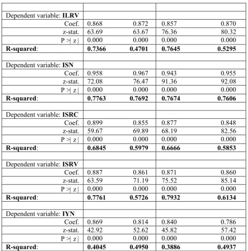
Table 8 shows the results for the time period 1985-2008 and the two panels, one with 14 EU
countries and the other including three non-EU countries. The comparison with the results reported
in the previous table highlights the increasing importance of the approximation mainly of the
nominal long-term and short-term interest rates series, but to some extent also of the yield curves
to the German patterns, as a consequence of the EMU and the single monetary policy.
A more attentive observation of the series of real interest rates also reveals that those using the
GDP deflator follow the German values more closely than those using the private consumption
deflator, particularly in the long term. This may be accepted as another symptom of the increasing
influence of the German patterns and not only on the interest rate series, but also and more clearly
on the GDP deflator patterns.
Table 8 – Three-stage panel estimations -
1985-2008
Variables * EU14** EU14+Japan+Norway+USA ∆Germany ∆USA ∆Germany ∆USA Dependent variable: ILN
Coef. 0.972 1.005 0.968 0.985 z-stat. 81.38 71.23 106.0 92.79 P >| z | 0.000 0.000 0.000 0.000
R-squared: 0.8571 0.8000 0.8536 0.7918
Dependent variable: ILRC
Coef. 0.878 0.865 0.859 0.854 t-stat. 59.29 59.78 67.66 74.81 P >| t | 0.000 0.000 0.000 0.000
20
Dependent variable: ILRV
Coef. 0.868 0.872 0.857 0.870 z-stat. 63.69 63.67 76.36 80.32 P >| z | 0.000 0.000 0.000 0.000
R-squared: 0.7366 0.4701 0.7645 0.5295
Dependent variable: ISN
Coef. 0.958 0.967 0.943 0.955 z-stat. 72.08 76.47 91.36 92.08 P >| z | 0.000 0.000 0.000 0.000
R-squared: 0.7763 0.7692 0.7674 0.7606
Dependent variable: ISRC
Coef. 0.899 0.855 0.877 0.848 z-stat. 59.67 69.89 68.19 82.56 P >| z | 0.000 0.000 0.000 0.000
R-squared: 0.6845 0.5979 0.6666 0.5853
Dependent variable: ISRV
Coef. 0.887 0.861 0.871 0.860 z-stat. 63.59 71.19 75.52 85.14 P >| z | 0.000 0.000 0.000 0.000
R-squared: 0.7761 0.5726 0.7932 0.6134
Dependent variable: IYN
Coef. 0.869 0.814 0.840 0.786 z-stat. 42.92 52.62 45.82 57.42 P >| z | 0.000 0.000 0.000 0.000
R-squared: 0.4045 0.4950 0.3886 0.4937
*
ILN = Nominal long-term interest rates; ILRC = Real long-term interest rates, deflator private consumption; ILRV = Real long-term interest rates, deflator GDP; ISN = Nominal short-term interest rates; ISRC = Real short-term interest rates, deflator private consumption; ISRV = Real short-term interest rates, deflator GDP; IYN = Yield curve; ∆ILN Germany = (ILN)i – (ILN)Germany; ∆ILRC Germany = (ILRC)i – (ILRC)Germany; ∆ILRV Germany = (ILRV)i – (ILRV)Germany; ∆ISN Germany = (ISN)i – (ISN)Germany; ∆ISRC Germany = (ISRC)i – (ISRC)Germany; ∆ISRV Germany = (ISRV)i – (ISRV)Germany; ∆IYN Germany = (IYN)i – (IYN)Germany; ∆ILN USA= (ILN)i – (ILN)USA; ∆ILRC USA= (ILRC)i – (ILRC) USA; ∆ILRV USA= (ILRV)i – (ILRV) USA; ∆ISN USA= (ISN)i – (ISN) USA; ∆ISRC USA= (ISRC)i – (ISRC) USA; ∆ISRV USA= (ISRV)i – (ISRV) USA ; ∆IYN USA= (IYN)i – (IYN) USA.
** EU-14 = Austria, Belgium, Denmark, Finland, France, Germany, Greece, Ireland, Italy, Netherlands, Portugal, Spain, Sweden, United Kingdom.
Table 9 presents the results obtained with three-stage panel estimates for our last two panels, i.e.,
those for the time period after the implementation of the EMU (1999-2008). Taking into account
the recent large-scale enlargement process, one of these panels includes 25 EU countries, while the
other adds four other non-EU countries.
Now the differences in the dynamics of the approximations towards the two chosen benchmarks
are much more evident. For the long-term nominal and real interest rates, the approximation of the
countries’ rates towards the US rates is almost as important as the approximation towards the
German rates. However, for the short-term nominal and real interest rates, as well as for the yield
21
Table 9 – Three-stage panel estimations -
1999-2008
Variables * EU25**
EU25+
+Japan+Norway+Switzerland+USA ∆Germany ∆USA ∆Germany ∆USA Dependent variable: ILN
Coef. 0.985 0.975 0.944 0.973 z-stat. 134.2 106.2 154.2 105.5 P >| z | 0.000 0.000 0.000 0.000
R-squared: 0.8263 0.7819 0.8530 0.8097
Dependent variable: ILRC
Coef. 0.984 0.964 0.982 0.946 t-stat. 151.1 90.95 166.0 86.87 P >| t | 0.000 0.000 0.000 0.000
R-squared: 0.8184 0.7112 0.8004 0.6822
Dependent variable: ILRV
Coef. 0.978 0.963 0.974 0.942 z-stat. 170.3 83.46 170.9 83.84 P >| z | 0.000 0.000 0.000 0.000
R-squared: 0.7873 0.7983 0.7892 0.7920
Dependent variable: ISN
Coef. 0.985 0.946 0.984 0.945 z-stat. 179.9 79.91 185.9 81.35 P >| z | 0.000 0.000 0.000 0.000
R-squared: 0.8526 0.5710 0.8599 0.5945
Dependent variable: ISRC
Coef. 0.983 0.932 0.981 0.921 z-stat. 171.1 69.08 182.7 69.78 P >| z | 0.000 0.000 0.000 0.000
R-squared: 0.8398 0.5710 0.8289 0.4632
Dependent variable: ISRV
Coef. 0.980 0.945 0.977 0.928 z-stat. 183.9 74.02 182.8 73.43 P >| z | 0.000 0.000 0.000 0.000
R-squared: 0.8037 0.4897 0.8020 0.5814
Dependent variable: IYN
Coef. 0.981 0.888 0.978 0.880 z-stat. 147.5 49.00 144.5 50.45 P >| z | 0.000 0.000 0.000 0.000
R-squared: 0.6949 0.3020 0.6767 0.2776
*
ILN = Nominal long-term interest rates; ILRC = Real long-term interest rates, deflator private consumption; ILRV = Real long-term interest rates, deflator GDP; ISN = Nominal short-term interest rates; ISRC = Real short-term interest rates, deflator private consumption; ISRV = Real short-term interest rates, deflator GDP; IYN = Yield curve; ∆ILN Germany = (ILN)i – (ILN)Germany; ∆ILRC Germany = (ILRC)i – (ILRC)Germany; ∆ILRV Germany = (ILRV)i – (ILRV)Germany; ∆ISN Germany = (ISN)i – (ISN)Germany; ∆ISRC Germany = (ISRC)i – (ISRC)Germany; ∆ISRV Germany = (ISRV)i – (ISRV)Germany; ∆IYN Germany = (IYN)i – (IYN)Germany; ∆ILN USA= (ILN)i – (ILN)USA; ∆ILRC USA= (ILRC)i – (ILRC) USA; ∆ILRV USA= (ILRV)i – (ILRV) USA; ∆ISN USA= (ISN)i – (ISN) USA; ∆ISRC USA= (ISRC)i – (ISRC) USA; ∆ISRV USA= (ISRV)i – (ISRV) USA ; ∆IYN USA= (IYN)i – (IYN) USA.
22
6. Concluding remarks
This paper applies “first” and “second” generation panel unit root and cointegration tests, as well
as panel fixed-effects and three-stage panel estimates, using the available AMECO series of
nominal and real long-term and short-term interest rates and yield curves covering the time period
between 1961 and 2008.
The results obtained for six panels of EU and some non-EU countries for three specific time
intervals allow us to conclude that:
1) In our six panels there is clear evidence of financial integration and, if we
consider that the approximation of the countries’ rates towards the US rates and yield
curves is representative of the global financial integration while the approximation
towards the German rates and yield curves represents European integration, we can
conclude that there is a specific process of European integration which is, for most EU
countries, much more relevant than the global process of integration.
2) The patterns of this approximation vary not only with the homogeneity of the
panel countries, but also with the considered time interval. More precisely, while the
implementation of the Single Market Program does not seem to be relevant to the
increase of the integration process, the EMU and the adoption of the single monetary
policy has enhanced European financial integration between EU countries, even
between those countries outside the euro area.
3) With regard to the differences in the patterns of approximation towards the
benchmarks of the individual series, there is clear evidence of the particular
characteristics of the yield curves: like almost all the other series, they are always
stationary and cointegrated series, but the approximation is not only with the German,
but also with the US yield curves. Generally speaking, the approximation towards the
German rates is more evident for the long-term than for the short-term interest rates.
This is particularly true for our first panels, which include quite homogeneous countries
during the entire time interval (1961-2008). The differences between nominal and real
interest rates also depend mainly on the homogeneity of the panel countries’ economies
23
References
Adam, K., T. Jappelli, A. M. Menichini, M. Padula and M. Pagano (2002) Analyse, Compare, and Apply Alternative Indicators and Monitoring Methodologies to Measure the
Evolution of Capital Market Integration in the European Union, Report to the European
Commission.
Adjaouté, K. and J.-P Danthine (2003) “European Financial Integration and Equity Returns: A Theory-Based Assessment”, in Gaspar, V. et al. (eds.) The transformation of the European financial system, ECB, Frankfurt.
Affinito, M. and F. Farabullini (2006) An empirical analysis of national differences in the retail bank interest rates of the euro area, Banca d’Italia, Temi di discussione, No. 589.
Baele, L., A. Ferrando, P. Hordahl, E. Krylova and C. Monnet (2004) Measuring financial integration in the euro area, ECB Working Paper Series No. 14.
Baier, S. L. and J. H. Bergstrand (2007) “Do free trade agreements actually increase members' international trade?” Journal of International Economics, Vol. 71 (1), pp. 72-95.
Cabral I., F. Dierick, and J. Vesala (2002) Banking Integration in the Euro Area, ECB Occasional Paper Series No. 6.
Dooley, M. P. (1996) "A Survey of Literature on Controls over International Capital Transactions," IMF Staff Papers, Vol. 43 (4), pp. 639- 687.
European Central Bank (2003) The integration of Europe’s financial markets, Monthly Bulletin, October.
European Central Bank (2007) Financial integration in Europe.
European Central Bank (2008) Financial integration in Europe.
Gardener, E.P.M., Ph. Molyneux and B. Moore (ed.) (2002) Banking in the New Europe –
The Impact of the Single Market Program and EMU on the European Banking Sector, Palgrave,
Macmillan.
Gropp, R. and A. K. Kashyap (2008) A New Metric for Banking Integration in Europe, paper presented at the NBER summer institute pre-conference and the 2nd ZEW conference on banking integration and stability.
Hartmann P., A. Maddaloni and S. Manganelli (2003) “The euro area financial system: structure integration and policy initiatives” Oxford Review of Economic Policy, Spring 2003, Vol.19 (1), pp. 180-213.
Im, K., M. Pesaran and Y. Shin (2003), “Testing for Unit Roots In Heterogeneous Panels”, Journal of Econometrics, No. 115, p. 53-74.
Levin, A, C. Lin and C. Chu (2002), “Unit Root Tests in Panel Data: Asymptotic and Finite Sample Properties”, Journal of Econometrics, No.108, p.1-24.
Maggi, G. (1999) “The Role of Multilateral Institutions in International Trade Cooperation” The American Economic Review, Vol. 89 (1), pp. 190-214.
Mansfiel, E.D., H. V. Milner and B. P. Rosendorff (2000) “Free to Trade: Democracies, Autocracies, and International Trade” The American Political Science Review, Vol. 94 (2), pp. 305-321. .
24 Obstfeld, M. (1998) “The Global Capital Market: Benefactor or Menace?” Journal of EconomicPerspectives, Vol. 12 (4), pp. 9–30.
Pesaran, M. H. (2004) “General diagnostic tests for cross-section dependence in panels”, Cambridge Working Papers in Economics, 0435, University of Cambridge.
Rose, A.K. and E. Wincoop (2001) “National Money as a Barrier to International Trade: The Real Case for Currency Union” The American Economic Review, Vol. 91 (2), pp. 386-390.
Sander, H. and S. Kleimeier (2004) “Convergence in euro-zone retail banking? What interest rate pass-through tells us about monetary policy transmission, competition and integration”, Journal of International Money and Finance, Vol. 23 , pp. 461–492.
Sørensen, C. K. and Gutiérrez J. M. P. (2006) Euro area banking sector integration using hierarchical cluster analysis techniques, ECB Working Paper Series No. 627.
Vajanne, L. (2007) Integration of euro area retail banking markets – convergence of credit interest rates, Bank of Finland Research Discussion Papers, N. 27.
Westerlund, J. (2007) “Testing for error correction in panel data” Oxford Bulletin of Economics and Statistics, Vol. 69, pp. 709-748.
25
Appendix I - Levin, Lin and Chu (2002) (LEVINLIN) panel unit root tests
LEVINLIN - 1961-2008
Variables *
EU9 (1961-2008)
EU9+USA (1961-2008) t-star P > t obs. t-star P > t obs.
ILN -0.75970 0.2237 368 -1.04387 0.1483 414 ILRC -5.96697 0.0000 376 -6.86974 0.0000 423 ILRV -6.13529 0.0000 376 -7.02770 0.0000 423 ISN -4.54645 0.0000 376 -5.00324 0.0000 423 ISRC -7.87296 0.0000 376 -8.00135 0.0000 423 ISRV -7.26727 0.0000 376 -7.61572 0.0000 423 IYN -8.13542 0.0000 376 -8.07926 0.0000 423
∆ILN Germany -0.83679 0.2014 368 -1.18102 0.1188 414 ∆ILRC Germany -5.99035 0.0000 376 -6.88126 0.0000 423 ∆ILRV Germany -6.03509 0.0000 376 -6.92702 0.0000 423 ∆ISN Germany -4.43818 0.0000 376 -4.92525 0.0000 423 ∆ISRC Germany -7.86370 0.0000 376 -8.03380 0.0000 423 ∆ISRV Germany -7.14578 0.0000 376 -7.55561 0.0000 423 ∆IYN Germany -7.82897 0.0000 376 -7.85386 0.0000 423 ∆ILN USA -0.68334 0.2472 376 -0.86324 0.1940 405 ∆ILRC USA -3.10117 0.0010 368 -3.62936 0.0001 414 ∆ILRV USA -3.80741 0.0001 368 -4.46746 0.0000 414 ∆ISN USA -3.41381 0.0003 368 -4.69192 0.0000 414 ∆ISRC USA -3.99903 0.0000 368 -4.28832 0.0000 414 ∆ISRV USA -4.13193 0.0000 368 -4.58329 0.0000 414 ∆IYN USA -4.13193 0.0000 368 -5.93755 0.0000 414
LEVINLIN - 1985-2008
Variables *
EU14 (1985-2008)
EU14+Japan+Norway+USA (1985-2008) t-star P > t obs. t-star P > t obs.
ILN -5.31051 0.0000 299 -6.20477 0.0000 368 ILRC -8.13703 0.0000 299 -8.05185 0.0000 368 ILRV -5.96812 0.0000 299 -6.42116 0.0000 368 ISN -4.13603 0.0000 299 -4.54063 0.0000 368 ISRC -6.81974 0.0000 299 -7.13969 0.0000 368 ISRV -6.04203 0.0000 299 -6.87373 0.0000 368 IYN -6.44178 0.0000 299 -6.09136 0.0000 368
26 LEVINLIN - 1999-2008
Variables * EU25 (1999-2008)
EU25+
+Japan+Norway+Switzerland+USA (1999-2008)
t-star P > t obs. t-star P > t obs.
ILN -6.59900 0.0000 216 -7.70370 0.0000 252
ILRC -5.80074 0.0000 192 -4.05149 0.0000 252
ILRV -3.14460 0.0008 216 -4.47915 0.0000 252
ISN -21.62761 0.0000 216 -19.96764 0.0000 252
ISRC -7.70508 0.0000 216 -9.42141 0.0000 252
ISRV -6.28570 0.0000 216 -7.49861 0.0000 252
IYN -8.55931 0.0000 216 -7.26688 0.0000 252
∆ILN Germany -5.70611 0.0000 216 -6.69823 0.0000 252
∆ILRC Germany -5.21726 0.0000 192 -4.34660 0.0000 252
∆ILRV Germany -3.52325 0.0002 216 -4.69526 0.0000 252
∆ISN Germany -16.56702 0.0000 216 -16.75886 0.0000 252
∆ISRC Germany -7.72367 0.0000 216 -9.21705 0.0000 252
∆ISRV Germany -8.14994 0.0000 216 -8.99967 0.0000 252
∆IYN Germany -7.30959 0.0000 216 -6.53823 0.0000 252
∆ILN USA -11.17996 0.0000 168 -5.38730 0.0000 224
∆ILRC USA -34,46709 0.0000 144 -5.08081 0.0000 224
∆ILRV USA -8.47538 0.0000 144 -12.10523 0.0000 224
∆ISN USA -6.78116 0.0000 144 -5.09249 0.0000 196
∆ISRC USA -7.15322 0.0000 144 -14.55328 0.0000 168
∆ISRV USA -29.01531 0.0000 144 -10.10851 0.0000 224
∆IYN USA -10.97404 0.0000 192 -9.58694 0.0000 224
Appendix II - Im, Pesaran and Shin (2003) (IPSHIN) panel unit root tests IPSHIN - 1961-2008 Variables * EU9 (1961-2008) EU9+USA (1961-2008) W[t-bar] P-value obs. W[t-bar] P-value obs. ILN -1.215 0.112 368 -1.525 0.064 405
ILRC -6.298 0.000 376 -7.204 0.000 423
ILRV -6.589 0.000 376 -7.608 0.000 423
ISN -4.450 0.000 376 -4.944 0.000 423
ISRC -7.821 0.000 376 -7.851 0.000 423
ISRV -7.247 0.000 376 -7.625 0.000 423
IYN -7.861 0.000 376 -7.792 0.000 423
∆ILN Germany -1.115 0.132 368 -1.500 0.067 405
∆ILRC Germany -6.269 0.000 376 -7.133 0.000 423
∆ILRV Germany -6.481 0.000 376 -7.475 0.000 423
∆ISN Germany -4.203 0.000 376 -4.728 0.000 423
∆ISRC Germany -7.859 0.000 376 -7.912 0.000 423
∆ISRV Germany -7.158 0.000 376 -7.573 0.000 423
∆IYN Germany -7.498 0.000 376 -7.511 0.000 423
∆ILN USA -1.170 0.121 360 -1.472 0.071 414
∆ILRC USA -3.924 0.000 368 -4.543 0.000 414
∆ILRV USA -4.809 0.000 368 -5.669 0.000 414
∆ISN USA -3.583 0.000 368 -4.938 0.000 414
∆ISRC USA -4.601 0.000 368 -4.808 0.000 414
∆ISRV USA -4.792 0.000 368 -5.278 0.000 414