Nome Completo do(a) Candidato(a)
(Tipo de letra: Arial, 14 pt negrito)Habilitações Académicas
(Tipo de letra: Arial, 11 pt normal)
Título da Dissertação
(Tipo de letra: Arial, 16 pt negrito)
Dissertação para obtenção do Grau de Doutor em
Nome do Curso
(Tipo de letra: Arial, 11 pt normal)
Orientador: Nome, Categoria, Escola Co-orientador: Nome, Categoria, Escola
(Tipo de letra: Arial, 12 pt normal)
Júri: (Font: Arial, 10 pt normal)
Presidente: Prof. Doutor(a) Nome Completo Arguente(s): Prof. Doutor(a) Nome Completo
Vogais: Prof. Doutor(a) Nome Completo Prof. Doutor(a) Nome Completo
Prof. Doutor(a) Nome Completo
(Tipo de letra: Arial, 10 pt normal)
Mês e Ano
(Tipo de letra: Arial, 11 pt negrito)
Cláudia Alexandra Rocha Ferreira
Mestre em Engenharia Civil
Use of Petri Nets to Manage
Civil Engineering Infrastructures
Dissertação para obtenção do Grau de Doutor em Engenharia Civil, Especialidade de Estruturas
Orientador: Luís Armando Canhoto Neves,
Professor Auxiliar, FCT/UNL
Co-orientador: José António Campos e Matos,
Professor Auxiliar, EEUM
Júri:
Presidente: Doutor Fernando Manuel Anjos Henriques Arguentes: Doutor Jorge Manuel Caliço Lopes de Brito
Doutor Luís Miguel Pina de Oliveira Santos Vogais: Doutor António Abel Henriques
Doutora Maria Paulina Santos Forte Faria Rodrigues Doutor Eduardo Soares Ribeiro Gomes Cavaco Doutor Luís Armando Canhoto Neves
i
Use of Petri Nets to Manage Civil Engineering Infrastructures
Copyrightc Cláudia Alexandra Rocha Ferreira, Faculdade de Ciências e Tecnologia, Universidade
Nova de Lisboa
iii
Acknowledgements
The completion of this dissertation represents the culmination of an important stage in my life. Its elaboration had the direct and indirect contribution of several people and entities, to which I am deeply grateful.
First and foremost, I would like to express my sincere gratitude to my supervisor, Dr. Luís Neves, for giving me the opportunity to do this work and for the confidence that has always shown from the first day. Without him, this work would not have been possible. For his constant support, friendship, guidance and sharing of knowledge’s throughout the entire work, I am truly grateful.
I also would like to express my deeply gratitude to Dr. José Campos e Matos, my co-supervisor, for his support, help and interest over the last few years.
I would also like to extend my thanks to Eng. Ugo Berardinelli, from Ascendi, and to Eng. Luís Marreiro, from BRISA, for all the support and help concerning the access of data relative bridges and road networks needed to carry out this work. As well as, to Dr. Ana Silva for helping with the ceramic claddings.
My appreciation goes also to the members of the Nottingham Transportation Engineering Centre (NTEC) of University of Nottingham for their friendship and how well I have been received. Thanks to all who made my time more enjoyable.
I acknowledge the financial support of theFundação para a Ciência e a Tecnologia, through the PhD
scholarship SFRH/BD/88195/2012.
The support of Civil Engineering Department ofFaculdade de Ciências e Tecnologiais greatly
ac-knowledged. I want to thank all Professor and researchers who helped me and supported me at various stages of this journey. I also would like to thank Maria da Luz and Carla for all helpful support that they gave me. Finally, to my colleagues, I want to thank for their friendship, support, share of ideas, mutual help, and fun over these years. With special thanks to Filipe, Nuno, Hugo and Renato.
I am sincerely grateful to my friends Andreia, Helena and Mafalda for their constant motivation, for being always by my side through good and bad times and above all for wanting me to realize my dreams. I am also truly grateful to Ana Rita for all her help in developing the thesis.
Finally, I wish to thank to my family, parents and sister, for their unconditional love, care and under-standing during this period. To them, I am deeply grateful.
Abstract
Over the last years there has been a shift, in the most developed countries, in investment and efforts within the construction sector. On the one hand, these countries have built infrastructures able to respond to current needs over the last decades, reducing the need for investments in new infrastruc-tures now and in the near future. On the other hand, most of the infrastrucinfrastruc-tures present clear signs of deterioration, making it fundamental to invest correctly in their recovery. The ageing of infrastructure together with the scarce budgets available for maintenance and rehabilitation are the main reasons for the development of decision support tools, as a mean to maximize the impact of investments.
The objective of the present work is to develop a methodology for optimizing maintenance strategies, considering the available information on infrastructure degradation and the impact of maintenance in economic terms and loss of functionality, making possible the implementation of a management system transversal to different types of civil engineering infrastructures. The methodology used in the deterioration model is based on the concept of timed Petri nets. The maintenance model was built from the deterioration model, including the inspection, maintenance and renewal processes. The optimization of maintenance is performed through genetic algorithms.
The deterioration and maintenance model was applied to components of two types of infrastructure: bridges (pre-stressed concrete decks and bearings) and buildings (ceramic claddings). The complete management system was used to analyse a section of a road network. All examples are based on Portuguese data.
Keywords: Infrastructure Management Systems; Petri nets; Deterioration; Maintenance; Optimiza-tion.
Resumo
Ao longo dos últimos anos, nos países mais desenvolvidos, tem-se assistido a um redirecionamento dos investimentos e dos esforços no sector da construção. Por um lado, estes países, construíram ao longo das últimas décadas infraestruturas capazes de responder às necessidades atuais, dimin-uindo a necessidade de investimentos em novas infraestruturas no presente e no futuro próximo, por outro, grande parte das infraestruturas existentes apresenta sinais claros de deterioração, tornando-se fundamental investir corretamente na recuperação das mesmas. Assim tornando-sendo, o envelhecimento das infraestruturas juntamente com os escassos orçamentos disponíveis para a realização de ações de manutenção e de reabilitação são os principais motivos para o desenvolvimento de ferramentas de apoio à decisão, como meio de maximizar os investimentos.
O presente trabalho tem como objetivo desenvolver uma metodologia de otimização de estratégias de manutenção considerando a informação disponível sobre a degradação das infraestruturas e o impacte das ações de manutenção em termos económicos e de perda de funcionalidade, possibilitando, desse modo, a implementação de um sistema de gestão transversal a diferentes tipos de infraestruturas de engenharia civil. A metodologia utilizada no modelo de deterioração é baseada no conceito de redes de Petri temporais. O modelo de manutenção foi construído a partir do modelo de deterioração, incluído os processos de inspeção, manutenção e renovação. A otimização das ações de manutenção é realizada através de algoritmos genéticos.
O modelo de deterioração e de manutenção foram aplicados a componentes de dois tipos de infraestru-turas: obras de arte (tabuleiros de betão armado e pré-esforçado, e aparelhos de apoio) e edifícios (revestimentos cerâmicos). O sistema de gestão completo foi utilizado para analisar um troço de uma rede rodoviária. Todos os exemplos apresentados são baseados em dados portugueses.
Palavras-chave: Sistemas de gestão de infraestruturas; Redes de Petri; Deterioração; Ações de manutenção; Otimização.
Contents
Abstract vii
Resumo ix
List of Figures xv
List of Tables xxi
Nomenclature xxv
1 Introduction 1
1.1 Background and motivation . . . 1
1.2 Objectives . . . 2
1.3 Methodology . . . 3
1.4 Outline of the dissertation . . . 5
2 Literature Review 7 2.1 Introduction . . . 7
2.2 Infrastructure management system . . . 8
2.2.1 Main components . . . 9
2.2.1.1 Database . . . 9
2.2.1.2 Deterioration model . . . 10
2.2.1.3 Optimization model . . . 11
2.2.1.4 Update . . . 11
2.2.2 Examples of infrastructure management systems . . . 12
2.2.2.1 Bridge management system . . . 12
2.2.2.2 Pavement management system . . . 16
2.2.2.3 Building management system . . . 18
2.2.2.4 Waterwaste management systems . . . 19
2.2.2.5 Other types of management systems . . . 19
2.3 Deterioration models . . . 20
2.4 Reliability-based deterioration models . . . 21
2.5 Condition-based deterioration models . . . 22
2.5.1 Markov chain-based models . . . 22
2.5.1.1 Discrete time Markov chains . . . 23
2.5.1.2 Continuous time Markov chains . . . 26
2.5.1.3 Background on Markov chain-based deterioration models . . . 28
2.5.2 Petri net-based models . . . 31
2.5.2.1 Original concept of Petri nets . . . 31
2.5.2.2 Background on Petri net-based deterioration models . . . 33
2.6 Maintenance . . . 34
2.6.1 Reliability-based models . . . 34
2.6.2 Condition-based models . . . 36
2.6.2.1 Markov chain-based models . . . 36
2.6.2.2 Petri net-based models . . . 37
2.7 Summary . . . 39
3 Petri Nets Theory 41 3.1 Introduction . . . 41
3.2 Extensions of the Petri nets . . . 41
3.2.1 Timed Petri nets . . . 41
3.2.2 Stochastic Petri nets . . . 42
3.2.3 Continuous timed Petri nets . . . 45
3.2.4 Coloured Petri nets . . . 45
3.3 Petri net component nomenclature . . . 47
3.3.1 Transitions and places . . . 47
3.3.2 Inhibitor arc . . . 48
3.4 Conflicts . . . 49
3.5 Summary . . . 51
4 Petri Net Model 53 4.1 Introduction . . . 53
4.2 Petri net deterioration model . . . 53
4.2.1 Estimation of the firing rates . . . 54
4.2.2 Monte Carlo simulation . . . 54
4.2.3 Genetic algorithm optimization . . . 56
4.3 Petri net maintenance model . . . 58
4.3.1 Inspection process . . . 58
4.3.2 Maintenance process . . . 59
4.3.3 Maintenance . . . 60
4.3.3.1 Effect of maintenance actions . . . 60
4.3.3.2 Modelling of maintenance actions . . . 61
4.3.3.3 Periodicity of the preventive maintenance . . . 64
4.3.4 Renewal process . . . 64
4.4 Complete maintenance model . . . 65
4.5 Computation of the performance profiles . . . 66
4.5.1 Performance profile without maintenance . . . 66
4.5.2 Performance profile with maintenance . . . 67
4.5.3 Cost of maintenance actions . . . 69
4.6 Summary . . . 69
5 Case Study 1: Application to Bridges 71 5.1 Introduction . . . 71
5.2 Classification system adapted . . . 71
5.3 Historical databases . . . 72
5.4 Validation of the Petri net deterioration model . . . 74
5.4.1 Markov chains deterioration model . . . 74
5.4.2 Pre-stressed concrete decks . . . 76
5.4.3 Bearings . . . 78
5.5 Probabilistic analysis . . . 81
5.5.1 Pre-stressed concrete decks . . . 81
5.5.2 Bearings . . . 85
CONTENTS xiii
5.6.1 Pre-stressed concrete decks . . . 91
5.6.2 Bearings . . . 96
5.7 Summary . . . 99
6 Case Study 2: Application to Ceramic Claddings 103 6.1 Introduction . . . 103
6.2 Classification of the degradation condition . . . 104
6.3 Probabilistic analysis . . . 104
6.4 Probabilistic analysis according to exposure . . . 109
6.4.1 Exposure to damp . . . 109
6.4.2 Distance from the sea . . . 111
6.4.3 Orientation . . . 112
6.4.4 Wind-rain action . . . 112
6.5 Statistical analysis . . . 113
6.6 Maintenance model . . . 115
6.6.1 Maintenance strategies . . . 117
6.6.2 Results . . . 118
6.7 Summary . . . 121
7 Case Study 3: Transportation Network 123 7.1 Introduction . . . 123
7.2 Resilience in transport networks . . . 123
7.2.1 Conceptual definition of resilience . . . 124
7.2.2 Analytical definition of resilience . . . 126
7.3 Traffic model . . . 131
7.3.1 Generic highway segment model . . . 131
7.3.2 On-ramp model . . . 132
7.3.3 Off-ramp model . . . 133
7.3.4 Origin segment model . . . 134
7.3.5 Destination segment model . . . 135
7.4 Description of the road network . . . 135
7.5 Calibration and validation of the traffic model . . . 135
7.5.1 Test network . . . 137
7.5.2 Calibration . . . 139
7.5.2.1 Case study A: Highway segments . . . 140
7.5.2.2 Case study B: Off-ramp segments . . . 141
7.5.2.3 Case study C: On-ramp segments . . . 144
7.5.2.4 Discussion of the results . . . 147
7.5.3 Validation . . . 154
7.5.3.1 Comparison of the fundamental parameters by section . . . 154
7.5.3.2 Comparison of the flow rate by node . . . 156
7.6 Performance evaluation of the road network . . . 156
7.6.1 Calculation ofΓ100 . . . 157
7.6.2 Calculation ofΓ0 . . . 158
7.6.3 Calculation ofΓfor other situations . . . 158
7.6.4 Discussion of the results . . . 158
7.7 Summary . . . 161
8 Multi-objective Optimization 163 8.1 Introduction . . . 163
8.2 Formulation of the optimization problem . . . 164
8.3.1 Optimization of performance indicators through the application of Mainte-nance D5 . . . 167
8.3.2 Optimization of performance indicators through the application of
Mainte-nances D4 and D5 . . . 169
8.3.3 Optimization of performance indicators through the application of
Mainte-nances D2, D4 and D5 . . . 172
8.3.4 Comparison of different optimal maintenance strategies for pre-stressed
con-crete decks . . . 176 8.4 Bearings . . . 177
8.4.1 Optimization of performance indicators through the application of
Mainte-nance B4 . . . 180
8.4.2 Optimization of performance indicators through the application of
Mainte-nances B4 and B3 . . . 187
8.4.3 Optimization of performance indicators through the application of
Mainte-nances B4, B3 and B2 . . . 192
8.4.4 Comparison of different optimal maintenance strategies for bearings . . . 195
8.5 Summary . . . 198
9 Conclusions and Future Developments 199
9.1 Conclusions . . . 199
9.2 Future developments . . . 203
References 205
A Definition of Places and Transitions 219
A.1 List of places . . . 219 A.2 List of transitions . . . 220
B Network Description 223
List of Figures
2.1 Life-cycle of an infrastructure . . . 9
2.2 Linear and non-linear reliability profiles without maintenance . . . 22
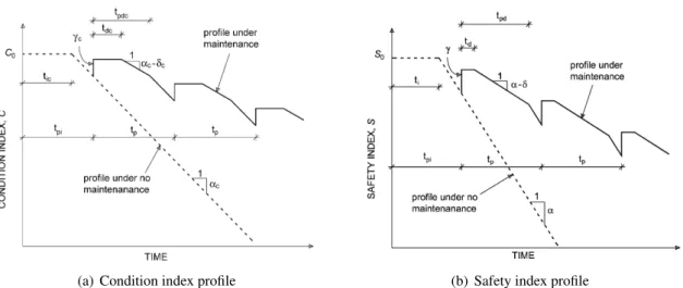
2.3 Condition and safety index profiles under no maintenance and under maintenance . . 23
2.4 Sample path of a discrete time Markov chain . . . 23
2.5 Sample path of a continuous time Markov chain . . . 27
2.6 Example of a Petri net . . . 31
2.7 Example of a transition (firing) rule . . . 32
2.8 Petri net scheme of the deterioration model . . . 33
2.9 Identification of the variables that describe the effects of preventive maintenance . . . 35
2.10 Maintenance model . . . 35
2.11 Markov state diagram for a single bridge element . . . 37
2.12 Petri net scheme of the maintenance model . . . 38
3.1 Petri net . . . 41
3.2 Example of a timed Petri net . . . 42
3.3 Example of a stochastic Petri net . . . 44
3.4 Reachability graph of the SPN . . . 44
3.5 Markov chain state space of the SPN . . . 44
3.6 Example of a continuous timed Petri net . . . 46
3.7 Simple example of a coloured Petri net . . . 46
3.8 Symbols often used to represent different types of transitions . . . 47
3.9 Symbols often used to represent different types of places . . . 48
3.10 Example of a Petri net with inhibitor arcs . . . 48
3.11 Example of a Petri net with conflict . . . 50
3.12 Example of a Petri net with conflict – Transition priority . . . 50
3.13 Example of a Petri net with conflict – Inhibitor arc . . . 50
3.14 Example of a Petri net with conflict – Alternate firing . . . 51
4.1 Petri net scheme of the deterioration model . . . 53
4.2 Procedure to compute the probability of occurrence of the observed transition . . . . 55
4.3 Procedure to optimize the parameters of probability distributions . . . 57
4.4 Introduction of the inspection process on the Petri net scheme of the maintenance model 58 4.5 Introduction of the maintenance process on the Petri net scheme of the maintenance model . . . 59
4.6 Effects of the maintenance actions . . . 62
4.7 Petri net scheme for preventive maintenance actions . . . 63
4.8 Petri net scheme for corrective maintenance actions . . . 63
4.9 Petri net scheme for periodicity of the preventive maintenance . . . 64
4.10 Petri net scheme of the complete maintenance process . . . 65
4.11 Procedure to compute the performance profile of the system over time horizon for the situation without maintenance . . . 66
4.12 Procedure to compute the performance profile of the system over time horizon for the
situation with maintenance . . . 68
5.1 Petri net scheme of the deterioration model for bridge components . . . 74
5.2 Comparison of the mean sojourn times for both methodologies in each condition state – Pre-stressed concrete decks . . . 77
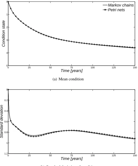
5.3 Comparison of the predicted future condition profile over time for both models – Pre-stressed concrete decks . . . 79
5.4 Comparison of the mean sojourn times for both methodologies in each condition state – Bearings . . . 79
5.5 Comparison of the predicted future condition profile over time for both models – Bearings . . . 80
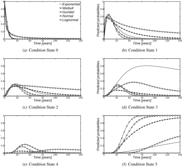
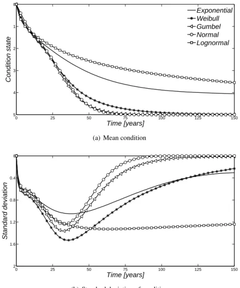
5.6 Comparison of the predicted future condition profile over time for all probability distribution analysed – Pre-stressed concrete decks . . . 83
5.7 Comparison of the probabilistic distribution for each condition state over time – Pre-stressed concrete decks . . . 84
5.8 Comparison of the predicted future condition profile over time for all probability distribution analysed – Bearings . . . 87
5.9 Comparison of the probabilistic distribution for each condition state over time – Bear-ings . . . 88
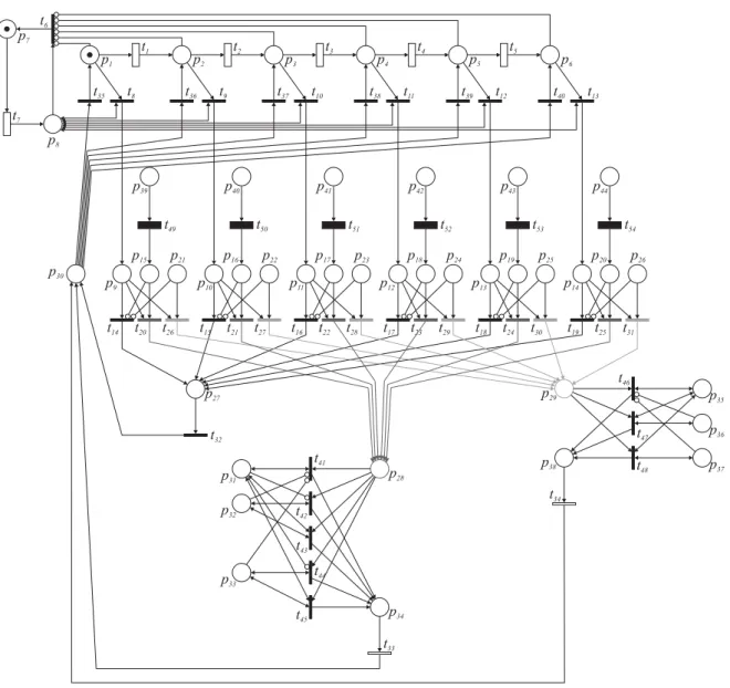
5.10 Petri net scheme of the maintenance model for bridges . . . 90
5.11 Comparison of the predicted future condition profile over time for all maintenance strategies considered – Pre-stressed concrete decks . . . 93
5.12 Cumulative cost profiles for three maintenance strategies considered. Black/green lines represent the mean cumulative cost and the gray/light green lines the standard deviation of the mean cumulative cost – Pre-stressed concrete decks . . . 94
5.13 Number of interventions for maintenance strategy 1 – Pre-stressed concrete decks . . 95
5.14 Number of interventions for maintenance strategy 2 – Pre-stressed concrete decks . . 95
5.15 Number of interventions for maintenance strategy 3 – Pre-stressed concrete decks . . 95
5.16 Percentiles of cumulative costs for the four maintenance strategies, whereC0.50,C0.90, C0.95, andC0.99 are the 50-, 90-, 95-, and 99-percentiles of the cumulative cost, re-spectively, considering an annual discount rate of 5% – Pre-stressed concrete decks . 96 5.17 Comparison of the predicted future condition profile over time for all maintenance strategies considered – Bearings . . . 98
5.18 Cumulative cost profiles for three maintenance strategies considered. Black lines represent the mean cumulative cost and the gray lines the standard deviation of the mean cumulative cost – Bearings . . . 99
5.19 Percentiles of cumulative costs for the three maintenance strategies, where C0.50, C0.90,C0.95, andC0.99are the 50-, 90-, 95-, and 99-percentiles of the cumulative cost, respectively, considering an annual discount rate of 5% – Bearings . . . 100
5.20 Number of interventions for maintenance strategy 1 – Bearings . . . 100
5.21 Number of interventions for maintenance strategy 2 – Bearings . . . 101
5.22 Number of interventions for maintenance strategy 3 – Bearings . . . 101
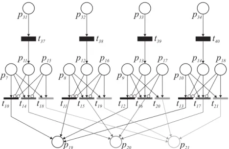
6.1 Petri net scheme of the deterioration model for claddings . . . 103
6.2 Comparison of the predicted future condition profile over time for all probability dis-tribution analysed. Mean and standard deviation are computed considering a corre-spondence between the condition scale and an integer scale between 1 and 5 . . . 107
6.3 Comparison of the probabilistic distribution for each condition state over time – Claddings . . . 108
6.4 Predicted future condition profile over time – Exposure to damp . . . 111
LIST OF FIGURES xvii
6.6 Predicted future condition profile over time – Orientation . . . 112
6.7 Predicted future condition profile over time – Wind-rain action . . . 113
6.8 Petri net scheme of the maintenance model for claddings . . . 116
6.9 Comparison of the predicted mean condition profile over time for all maintenance strategies considered. Mean and standard deviation are computed considering a cor-respondence between the condition scale and an integer scale between 1 and 5 . . . . 119
6.10 Cumulative cost profiles for three maintenance strategies considered. Black lines represent the mean cumulative cost and the gray lines the standard deviation of the mean cumulative cost . . . 122
7.1 Aspects of resilience . . . 125
7.2 Resilience triangle (shaded area); att=t0the external event occurs, and att=trthe recovery is complete . . . 126
7.3 Resilience according to Equation 7.3. The faster recovery path (dashed) yields a lower value of resilience (area with diagonal pattern) than the slower recovery path (solid) . 128 7.4 Resilience according to Equation 7.4. The faster recovery path (dashed) correctly yields a higher value of resilience (area with diagonal pattern) than the slower recov-ery path (solid) . . . 128
7.5 Resilience according to Equation 7.5. The numerator of Equation 7.5 is the shaded area, the denominator is the area of the large rectangle (area with diagonal pattern) . 129 7.6 Petri net scheme for a generic highway segment . . . 131
7.7 Petri net scheme for the on-ramp . . . 133
7.8 Petri net scheme for the off-ramp . . . 134
7.9 Petri net scheme for the origin segment . . . 134
7.10 Petri net scheme for the destination segment . . . 135
7.11 Implementation the network studied in the case study in the Portuguese highway net-work . . . 136
7.12 Scheme of the network . . . 136
7.13 Location of the sub-network . . . 137
7.14 Petri net scheme of the traffic model for the test network . . . 138
7.15 Generic relationships between speed, density and flow rate . . . 140
7.16 Comparison of the relationships between speed, density, and flow rate between the traffic model proposed by Tolba et al. (2005) and the data obtained from the Aimsun – Case study A . . . 141
7.17 Comparison of the relationships between speed, density, and flow rate between the traffic model proposed by Tolba et al. (2005) and the data obtain from the Aimsun – Case study B, Section 1 . . . 142
7.18 Comparison of the relationships between speed, density, and flow rate between the traffic model proposed by Tolba et al. (2005) and the data obtain from the Aimsun – Case study B, Section 2 . . . 142
7.19 Comparison of the relationships between speed, density, and flow rate between the traffic model proposed by Tolba et al. (2005) and the data obtain from the Aimsun – Case study B, Section 3 . . . 143
7.20 Comparison of the relationships between speed, density, and flow rate between the traffic model proposed by Tolba et al. (2005) and the data obtain from the Aimsun – Case study B, Section 4 . . . 143
7.21 Comparison of the relationships between speed, density, and flow rate between the traffic model proposed by Tolba et al. (2005) and the data obtain from the Aimsun – Case study C, Section 1 . . . 145
7.23 Comparison of the relationships between speed, density, and flow rate between the traffic model proposed by Tolba et al. (2005) and the data obtain from the Aimsun – Case study C, Section 3 . . . 146 7.24 Comparison of the relationships between speed, density, and flow rate between the
traffic model proposed by Tolba et al. (2005) and the data obtain from the Aimsun – Case study C, Section 5 . . . 146 7.25 First-degree polynomial used to describe the flow in uninterrupted conditions . . . . 148 7.26 Adjustment of the traffic model proposed to the data obtained from the Aimsun for
type 1 segments (Sections 1, 2, and 3 of case study A) . . . 150 7.27 Adjustment of the traffic model proposed to the data obtained from the Aimsun for
type 1 segments (Sections 1, 2, and 3 of case study B) . . . 150 7.28 Adjustment of the traffic model proposed to the data obtained from the Aimsun for
type 1 segments (Sections 1, and 2 of case study C) . . . 151 7.29 Adjustment of the traffic model proposed to the data obtained from the Aimsun for
type 2 segments (Section 3 of case study C) . . . 152 7.30 Adjustment of the traffic model proposed to the data obtained from the Aimsun for
type 3 segments (Section 5 of case study C) . . . 153 7.31 Adjustment of the traffic model proposed to the data obtained from the Aimsun for
type 4 segments (Section 4 of case study B) . . . 154 7.32 Scheme of the traffic flow circulation to the situation in which all bridges are in service 159 7.33 Identification of the sections in the road network . . . 160 7.34 Variation of the flow rate on the ramp between highway A9 and A10 in the South –
North direction (from Section 11 to Section 16) over time . . . 161
8.1 Example of a set of solutions and the first non-dominated front of a multi-objective
optimization problem . . . 164
8.2 Flowchart of the main interactions between the models of the tri-objective
optimiza-tion problem . . . 165
8.3 Flowchart of the main interactions between the models of the bi-objective
optimiza-tion problem . . . 166
8.4 Relationship between mean condition state and total maintenance cost at time horizon
– Maintenance D5 – Pre-stressed concrete decks . . . 167
8.5 Comparison of the design variable (time interval between major inspections, tinsp)
with the two objective functions (mean condition state and total maintenance cost at the time horizon) – Maintenance D5 – Pre-stressed concrete decks . . . 168
8.6 Comparison of the condition and cumulative cost profiles for solutions A, B, and C.
Solid lines represent the variation of the condition and cumulative cost profiles over time and the dashed lines the mean condition state – Maintenance D5 – Pre-stressed concrete decks . . . 169
8.7 Relationship between mean condition state and total maintenance cost at time horizon
– Maintenance D4 and D5 – Pre-stressed concrete decks . . . 170
8.8 Comparison of the design variable (time interval between major inspections, tinsp)
with the two objective functions (mean condition state and total maintenance cost at the time horizon) – Maintenance D4 and D5 – Pre-stressed concrete decks . . . 171
8.9 Comparison of the condition and cumulative cost profiles for solutions A, B, and C.
Solid lines represent the variation of the condition and cumulative cost profiles over time and the dashed lines the mean condition state – Maintenance D4 and D5 – Pre-stressed concrete decks . . . 172 8.10 Relationship between mean condition state and total maintenance cost at time horizon
– Maintenance D2, D4 and D5 – Pre-stressed concrete decks . . . 173 8.11 Non-dominated and dominated solutions – Maintenance D2, D4 and D5 – Pre-stressed
LIST OF FIGURES xix
8.12 Comparison of the design variable (time interval between major inspections, tinsp)
with the two objective functions (mean condition state and total maintenance cost at the time horizon) – Maintenance D2, D4 and D5 – Pre-stressed concrete decks . . . . 174 8.13 Comparison of the condition and cumulative cost profiles for solutions A, B, C and D.
Solid lines represent the variation of the condition and cumulative cost profiles over time and the dashed lines the mean condition state – Maintenance D2, D4 and D5 – Pre-stressed concrete decks . . . 175 8.14 Comparison of the condition and cumulative cost profiles for solutions C, C’, and C”.
Solid lines represent the variation of the condition and cumulative cost profiles over time and the dashed lines the mean condition state – Maintenance D2, D4 and D5 – Pre-stressed concrete decks . . . 176 8.15 Comparison of the dominated solutions of the three maintenance strategies –
Pre-stressed concrete decks . . . 177 8.16 Identification of the sections in the road network . . . 178 8.17 Relationship between three objective functions (mean condition state, total
mainte-nance cost at time horizon and resilience) – Maintemainte-nance B4 – Bearings . . . 180 8.18 Projections of the objective functions in bi-dimensional space – Maintenance B4 –
Bearings . . . 181
8.19 Comparison of the design variable (time interval between major inspections, tinsp)
with the three objective functions (mean condition state, total maintenance cost at the time horizon and resilience) – Maintenance B4 – Bearings . . . 182 8.20 Comparison of the condition, cumulative cost and resilience profiles for solutions with
shorter time intervals between major inspections for the six situations analysed. Solid lines represent the variation of the condition, cumulative cost and resilience profiles over time and the dashed lines the mean condition state and resilience, respectively – Maintenance B4 – Bearings . . . 183 8.21 Comparison of the condition, cumulative cost and resilience profiles for solutions with
intermediate time intervals between major inspections for the six situations analysed. Solid lines represent the variation of the condition, cumulative cost and resilience profiles over time and the dashed lines the mean condition state and resilience, re-spectively – Maintenance B4 – Bearings . . . 184 8.22 Comparison of the condition, cumulative cost and resilience profiles for solutions with
longer time intervals between major inspections for the six situations analysed. Solid lines represent the variation of the condition, cumulative cost and resilience profiles over time and the dashed lines the mean condition state and resilience, respectively – Maintenance B4 – Bearings . . . 185 8.23 Relationship between three objective functions (mean condition state, total
mainte-nance cost at time horizon and resilience) – Maintemainte-nance B4 and B3 – Bearings . . . 187 8.24 Projections of the objective functions in bi-dimensional space – Maintenance B4 and
B3 – Bearings . . . 188
8.25 Comparison of the design variable (time interval between major inspections, tinsp)
with the three objective functions (mean condition state, total maintenance cost at the time horizon and resilience) – Maintenance B4 and B3 – Bearings . . . 189 8.26 Comparison of the condition, cumulative cost and resilience profiles for all solutions.
Solid lines represent the variation of the condition, cumulative cost and resilience profiles over time and the dashed lines the mean condition state and resilience, re-spectively – Maintenance B4 and B3 – Bearings . . . 191 8.27 Relationship between three objective functions (mean condition state, total
mainte-nance cost at time horizon and resilience) – Maintemainte-nance B4, B3 and B2 – Bearings . 192 8.28 Projections of the objective functions in bi-dimensional space – Maintenance B4, B3
8.29 Comparison of the design variable (time interval between major inspections, tinsp) with the three objective functions (mean condition state, total maintenance cost at the time horizon and resilience) – Maintenance B4, B3 and B2 – Bearings . . . 194 8.30 Comparison of the condition, cumulative cost and resilience profiles for all solutions.
Solid lines represent the variation of the condition, cumulative cost and resilience profiles over time and the dashed lines the mean condition state and resilience, re-spectively – Maintenance B4, B3 and B2 – Bearings . . . 196 8.31 Comparison of the non-dominated solution of the three maintenance strategies –
Bear-ings . . . 197
B.1 Network analysed . . . 223 B.2 Petri net scheme of Section 1 of the network – Section (1) – (A) . . . 224 B.3 Petri net scheme of Section 2 of the network – Section (A) – (2) . . . 225 B.4 Petri net scheme of Section 3 of the network – Section (2) – (3) . . . 226 B.5 Petri net scheme of Section 4 of the network – Section (3) – (4) . . . 227 B.6 Petri net scheme of Section 5 of the network – Section (4) – (B) . . . 228 B.7 Petri net scheme of Section 6 of the network – Section (B) – (7) . . . 229 B.8 Petri net scheme of Section 7 of the network – Section (7) – (B) . . . 229 B.9 Petri net scheme of Section 8 of the network – Section (B) – (4) . . . 230 B.10 Petri net scheme of Section 9 of the network – Section (4) – (3) . . . 231 B.11 Petri net scheme of Section 10 of the network – Section (3) – (2) . . . 232 B.12 Petri net scheme of Section 11 of the network – Section (2) – (A) . . . 233 B.13 Petri net scheme of Section 12 of the network – Section (A) – (1) . . . 234 B.14 Petri net scheme of Section 13 of the network – Section (5) – (B) . . . 235 B.15 Petri net scheme of Section 14 of the network – Section (B) – (6) . . . 236 B.16 Petri net scheme of Section 15 of the network – Section (6) – (A) . . . 237 B.17 Petri net scheme of Section 16 of the network – Section (A) – (6) . . . 238 B.18 Petri net scheme of Section 17 of the network – Section (6) – (B) . . . 239 B.19 Petri net scheme of Section 18 of the network – Section (B) – (5) . . . 240 B.20 Petri net scheme of the intersection between A9 and A10 – Intersection (A) . . . 241 B.21 Petri net scheme of the intersection between A1 and A10 – Intersection (B) . . . 242 B.22 Scheme of the traffic flow circulation in the situation in which Sections 2 and 11 are
unavailable . . . 243 B.23 Scheme of the traffic flow circulation in the situation in which Sections 3 and 10 are
unavailable . . . 244 B.24 Scheme of the traffic flow circulation in the situation in which Sections 4 and 9 are
unavailable . . . 245 B.25 Scheme of the traffic flow circulation in the situation in which Sections 5 and 8 are
unavailable . . . 246 B.26 Scheme of the traffic flow circulation in the situation in which Sections 14 and 17 are
unavailable . . . 247 B.27 Scheme of the traffic flow circulation in the situation in which Sections 15 and 16 are
List of Tables
2.1 Evolution of the condition of the United States infrastructure systems over the years . 8
2.2 Condition rating used by NBI as a guide to evaluate bridge elements . . . 10
4.1 Variables used in the maintenance model for defining the application of maintenance
actions . . . 67
5.1 List of the bridge components . . . 72
5.2 Condition state for bridge components . . . 72
5.3 Example of a bridge with five inspections . . . 73
5.4 Division of Bridge B into two records . . . 73
5.5 Number of components and transitions for each bridge element . . . 73
5.6 Optimal parameters of the Markov chains deterioration model . . . 75
5.7 Observed and predicted values from both bridge components analysed . . . 76
5.8 Results of goodness-of-fit test,T . . . 76
5.9 Comparison of the optimal parameters of the Markov chains and Petri nets models –
Pre-stressed concrete decks . . . 77 5.10 Number of observed and predicted bridge components in each degradation condition
and the relative error obtained for both models – Pre-stressed concrete decks . . . 78
5.11 Comparison of the optimal parameters of the Markov chains and Petri nets models – Bearings . . . 78 5.12 Number of observed and predicted bridge components in each degradation condition
and the relative error obtained for both models – Bearings . . . 80 5.13 Probability density function . . . 81 5.14 Optimal parameters obtained for all probability distribution analysed in terms of mean
and standard deviation of time in each condition state – Pre-stressed concrete decks . 82
5.15 Number of observed and predicted pre-stressed concrete decks in each condition state for each probability distribution and relative error [%] obtained for each probability distribution – Pre-stressed concrete decks . . . 82 5.16 Optimal parameters obtained for all probability distribution analysed in terms of mean
and standard deviation of time in each condition state – Bearings . . . 85
5.17 Number of observed and predicted bearings in each condition state for each proba-bility distribution and relative error [%] obtained for each probaproba-bility distribution – Bearings . . . 85
5.18 Maintenance activities – Pre-stressed concrete decks . . . 89
5.19 Maintenance activities – Bearings . . . 89
5.20 Parameters of the Weibull distribution – Pre-stressed concrete decks . . . 92
5.21 Parameters of the Weibull distribution – Bearings . . . 97
6.1 Degradation conditions for ceramic claddings . . . 105
6.2 Optimal parameters obtained for all probability distribution analysed . . . 106
6.3 Number of observed and predicted claddings in each condition level for each proba-bility distribution and mean error obtained for each probaproba-bility distribution . . . 106
6.4 Comparison of the optimal parameters of the Markov chains and Petri nets models
(Exponential distribution) . . . 106
6.5 Probability of belonging to a condition as a function of the variables considered . . . 110
6.6 ANOVA test results . . . 114
6.7 Pairwise comparison . . . 115
6.8 Association of the risk with the extension of the defects and the maintenance actions
required . . . 117
6.9 Association of the risk with the extension of the defects and the maintenance actions
required . . . 117 6.10 Parameters of the Weibull distribution . . . 118 6.11 Number of interventions for maintenance strategy 1 . . . 119 6.12 Statistics of the time of the first intervention (in years) for maintenance strategy 1 . . 120 6.13 Number of interventions for maintenance strategy 2 . . . 120 6.14 Statistics of the time of the first intervention (in years) for maintenance strategy 2 . . 120 6.15 Number of interventions for maintenance strategy 3 . . . 121 6.16 Statistics of the time of the first intervention (in years) for maintenance strategy 3 . . 121 6.17 Maintenance cost . . . 121
7.1 Bridge functionality . . . 130 7.2 Network characteristics . . . 137 7.3 Test network characteristics . . . 138 7.4 Definition of places and transitions functions included in the traffic model for the test
network . . . 139
7.5 Input traffic flow [veh/h] data used in each simulation for the Case study A . . . 141
7.6 Input traffic flow [veh/h] data used in each simulation for the Case study B . . . 144
7.7 Input traffic flow [veh/h] data used in each simulation for the Case study C . . . 147
7.8 Type 1 segment characteristics . . . 149
7.9 Type 2 segment characteristics . . . 151
7.10 Type 3 segment characteristics . . . 152 7.11 Type 4 segment characteristics . . . 153 7.12 Origin-Destination matrix 1 (OD1) . . . 154 7.13 Origin-Destination matrix 2 (OD2) . . . 154 7.14 Origin-Destination matrix 3 (OD3) . . . 155 7.15 Origin-Destination matrix 4 (OD4) . . . 155 7.16 Comparison of the fundamental parameters in Section 1 . . . 155 7.17 Comparison of the fundamental parameters in Section 2 . . . 155 7.18 Comparison of the fundamental parameters in Section 3 . . . 155 7.19 Comparison of the fundamental parameters in Section 4 . . . 156 7.20 Comparison of the fundamental parameters in Section 5 . . . 156 7.21 Comparison of the flow rate [veh/h] in the bifurcation . . . 156 7.22 Comparison of the flow rate [veh/h] in the junction . . . 157 7.23 Daily traffic flow of the road network for January 20, 2014 . . . 157 7.24 Results: total travel time, total travel distance, performance network, functionality,
and resilience of the road network for each of the studied situations . . . 160
8.1 Mean number of intervention for solutions A, B, and C – Maintenance D5 –
Pre-stressed concrete decks . . . 168
8.2 Comparison of the performance indicators for solutions A, B, and C – Maintenance
LIST OF TABLES xxiii
8.3 Comparison of the performance indicators for solutions A, B, and C – Maintenance
D4 and D5 – Pre-stressed concrete decks . . . 170
8.4 Mean number of intervention for solutions A, B, and C – Maintenance D4 and D5 –
Pre-stressed concrete decks . . . 171
8.5 Comparison of the performance indicators for all solutions – Maintenance D2, D4
and D5 – Pre-stressed concrete decks . . . 173
8.6 Mean number of intervention for all solutions – Maintenance D2, D4 and D5 –
Pre-stressed concrete decks . . . 175
8.7 Average daily traffic flow of the road network on January 2014 . . . 178
8.8 Results: total travel time, total travel distance, performance network, and resilience
of the road network for the situation in which all bridges are in service . . . 178 8.9 Identification of the restricted segments in each section . . . 179 8.10 Results: total travel time, total travel distance, performance network, and resilience
of the road network for each of the studies situations . . . 179 8.11 Mean number of intervention for all solutions – Maintenance B4 – Bearings . . . 186 8.12 Comparison of the performance indicators for all solutions – Maintenance B4 – Bearings186 8.13 Comparison of the performance indicators for all solutions – Maintenance B4 and B3
– Bearings . . . 190 8.14 Mean number of intervention for all solutions – Maintenance B4 and B3 – Bearings . 190 8.15 Comparison of the performance indicators for all solutions – Maintenance B4, B3 and
B2 – Bearings . . . 195 8.16 Mean number of intervention for all solutions – Maintenance B4, B3 and B2 – Bearings195
Nomenclature
List of symbols
Upper Roman letters
A Total area of the façade
An Area of coating affected by an anomalyn
C Condition index
C(t) Time dependent condition index
Ci Vehicle capacity of the highway segmenti
C0 Initial condition index
D Incidence matrix for a Petri net composed only by ordinary arcs
D′ Incidence matrix for a Petri net composed by ordinary and inhibitor arcs
E Total number of elements present in the database
E(t) Expected value of the system condition at timet
Ei Expected number of transitions
FT Firing time
H(M) Inhibitor matrix
Ke Total number of transitions observed in the elementein the database
L Likelihood
Li Length of the highway segmenti
M Current marking of the Petri net
M(pi) Number of tokens in placepi
M′ New marking of the Petri net
Mi,Mj Generic marking of the Petri net
M0 Initial marking of the Petri net
MSE Within-groups mean squares in the ANOVA statistical test
MSR Between-groups mean squares in the ANOVA statistical test
N Total number of transition periods
Oi Observed number of transitions
P Transition probability matrix
P Finite set of places in the Petri net
P(·) Probability
P(·|·) Conditional probability
Pf Probability of failure
Post Post-incidence matrix in the Petri net
Pre Pre-incidence matrix in the Petri net
Q Transition intensity matrix
Q Load effect
Q(t) Percentage “functionality” (or “quality”, or “serviceability”) of the system at timet
R Resistance; Resilience
R(M0) Set of all markings which can be reached from the initial markingM0
RL Loss of resilience experienced by the system
RLog Logarithmic resilience
S Safety index; Vector of condition states defined in the performance scale
S(t) Time dependent safety index
Scri Critical speed
Sf ree i Limited maximum speed of the highway segmenti
Si(t) Average speed of the highway segmentiat timet
Sw Degradation severity of the coating
S0 Initial safety index
SSE Within-groups sum of squares in the ANOVA statistical test
SSR Between-groups sum of squares in the ANOVA statistical test
T Finite set of transitions in the Petri net; Goodness-of-fit test
Tj Mean sojourn time in condition state j
T T D(t) Total travel distance at timet T T T(t) Total travel time at timet
V Vector of transitions maximum firing speeds
X Set of nodes of the network
X(t) Condition state of the process at timet
NOMENCLATURE xxvii
Lower Roman letters
ci Time required to cover the highway segmentiwith traffic flow rateqi
ct Cost at timet
c0 Cost at present
d f Number of degrees of freedom
dj Delay associated with transitiontj in the Petri net
fi(t) Traffic flow rate entering the network at input pointiat timet
i Generic highway segment in the traffic model
k Multiplying factor; Total number of groups tested in the ANOVA statistical test
ka,n Weighting factor corresponding to the relative weight of the anomaly detected
ke Generic transition observed in the elementein the database
kn Multiplying factor of anomalyn, as a function of their degradation level
ˆ
l Normalized log-likelihood
logL Logarithm of the likelihood (log-likelihood)
lb(t) Bridge damage level at timet
m Total number of transitions in the Petri net
m′ Total number of timed transitions in the Petri net
mpi(t) Number of tokens in placepi at timet
n Total number of places in the Petri net; Total number of observations in each group
tested in the ANOVA statistical test
ni Total number of components in statei
ni j Total number of components transitioning from stateito state j
ni,nj Number of observations in groupiand jin the ANOVA statistical test
nMCS Total number of trials in the MCS
nMCS,j Number of trials in the MCS where the condition state predicted is equal to the condition
state observed, state j
ns Number of elements presents in the sample
p Randomly generated probability uniformly distributed between 0 and 1; Number of
estimated parameters
p(t) Condition vector at timet
pi Generic place in the Petri net
pi j Probability of transition from stateito state j
post(pi,tj) Post-condition of the transitiontj; Weight of the arc from transitiontj to placepi
pre(pi,tj) Pre-condition of the transitiontj; Weight of the arc from placepito transitiontj
qi(t) Average flow rate of the highway segmentiat timet
qi j Transition intensity from stateito state j
qmax i Maximum flow rate of transitioni
s Finite state space; Total number of condition states defined in the performance scale
t Time
td Time during which the deterioration process of performance level is suppressed
th Time horizon
ti,tI Instant of damage initiation; Generic transition in the traffic model
tinsp Time interval between major inspections
tinsp,max Upper limit of the time interval between major inspections
tinsp,min Lower limit of the time interval between major inspections
tj Generic transition in the Petri net
·tj Pre-set of places of the transitiontj
tP Time of reapplication of the maintenance
tpd,tPD Duration of the effect of the maintenance
tPI Application time of first maintenance
tr Time during which the deterioration rate of the performance level is affected; Time that
the recovery of the system is complete
t0 Time that external event occurs
∆t Time interval
u Firing vector
uj Firing frequency associated with transitiontjin the Petri net
v Annual discount rate
vi(t) Transition firing speed that represents the average flow rateqi(t)of the highway seg-menti
vj Firing speed associated with transitiontj in the Petri net
vmax i Maximum firing frequency of the highway segmenti
¯
yi,y¯j Mean of the groupiand jin the ANOVA statistical test
Upper Greek letters
Γ(t) Performance of the network at timet
Γ0 Value ofΓ(t)when none of bridges is in service
Γ100 Value ofΓ(t)when all bridges are in service
Θ Deterioration rate vector; Set of parameters of an arbitrary probabilistic distribution
NOMENCLATURE xxix
Φ(·) Cumulative distribution function of the standard normal variate
Lower Greek letters
α Deterioration rate of performance level without maintenance; Significance level
αi Maximum number of possible simultaneous firings associated with the highway
seg-menti
β Reliability index
β0 Initial reliability index
β(t) Time dependent reliability index
∆β Variation of the reliability index
γ Improvement of the performance level after the application of the maintenance
γD Balancing factor (cost) associated with the distance travelled by the users in the network
γT Balancing factor (cost) associated with the time spent by the users in the network
δ Deterioration factor
θ Deterioration rate of performance level during the effect of maintenance
θj Parameter of the probabilistic distribution associated with transitiontj
λj Scale parameter of the exponential distribution associated with condition state j; Firing
rate of the transitiontjthat transformsMiintoMj
µ(t) Mean of the condition state at timet
µcost(t) Mean of the cumulative maintenance cost at timet
νji Transition intensity back from state jto statei
ρcri Critical density
ρi(t) Average flow density of the highway segmentiat timet
ρmax i Jam density of the highway segmenti
σ(t) Standard deviation of the condition state at timet
σcost(t) Standard deviation of the cumulative maintenance cost at timet
τ Sojourn time
List of acronyms
AASHTO American Association of State Highway and Transportation Officials
ANOVA ANalysis Of VAriance
ASCE American Society of Civil Engineers
BdMS Building Management System
BREX Concrete Bridge Rating EXpert system
CDF Cumulative Distribution Function
CM Corrective Maintenance
CS Condition State
CTMC Continuous Time Markov Chains
CTPN Continuous Timed Petri Net
DSPN Deterministic and Stochastic Petri Net
DTMC Discrete Time Markov Chains
ESPN Extended Stochastic Petri Net
FCT Faculdade de Ciências e Tecnologia
FHWA Federal Highway Administration
GA Genetic Algorithm
GDP Gross Domestic Product
GSPN Generalized Stochastic Petri Net
iCDF Inverse Cumulative Distribution Function
IMS Infrastructure Management System
MC Markov Chain
MCS Monte Carlo Simulation
MR&R Maintenance, Repair and Rehabilitation
NBI National Bridge Inventory
NBIP National Bridge Inspection Program
NCHRP National Cooperative Highway Research Project
NDT Non-Destructive Tests
OD Origin-Destination matrix
OECD Organisation for Economic Co-operation and Development
PCI Pavement Condition Index
PDF Probability Density Function
PM Preventive Maintenance
PMS Pavement Management System
PN Petri Net
SPN Stochastic Petri Net
TPN Timed Petri Net
TSS Transport Simulation Systems
NOMENCLATURE xxxi
WMS Waterwaste Management System
2-D Two-Dimensional
Petri net symbology
Place
Continuous place
Directed arc
Bidirectional arc
Inhibitor arc
Immediate transition
Timed transition with deterministic time delay
Timed transition with stochastic time delay
Continuous timed transition
Reset transition
Chapter 1
Introduction
1.1
Background and motivation
The paradigm in the construction sector is changing. Economic aspects (ageing of the infrastruc-tures and the scarcity of funding for maintenance and rehabilitation actions) as well as environmental concerns (increase of awareness of the concept of sustainability and the environmental impact of the construction sector) are the main reasons for this change (Scherer and Glagola, 1994; Hovde, 2002; Paulo et al., 2014). This paradigm shift has resulted in an effort to develop decision support tools that maximize the benefits of the investments done in the past by extending the life of existing infrastructures. A more rational approach to decision-making in terms of inspection, maintenance and rehabilitation of the built heritage is required. For this purpose, several steps should be followed. Firstly, it is important to compile an inventory of existing structures and the conservation state of each structure. Secondly, it is essential to develop deterioration models to predict the future performance of these structures. After that, in a third stage, the development of maintenance and optimization models is fundamental to assess the impact of maintenance actions and to optimize better maintenance strate-gies. Over the past decades, a range of methods have been proposed in the literature for modelling deterioration maintenance and inspections (Thompson et al., 1998; Neves and Frangopol, 2005), as well as, method to optimize inspections and maintenance (Miyamoto et al., 2000; Yang et al., 2006).
The experience gained on the use of these models showed that the uncertainty associated with the deterioration process has to be explicitly included in the decision-making process, since the complex-ity of the phenomena involved and the limited information available make it impossible to model the deterioration with high precision (Lounis and Madanat, 2002). However, the main difficulty of all these methods is the fit of the inspection data, which is not absolutely reliable. According to Phares et al. (2004), visual inspections are an unreliable method for the evaluation of infrastructures con-servation state. Different inspectors under different conditions, evaluate significantly differently the conservation state of the infrastructure, introducing an additional source of uncertainty (Corotis et al., 2005).
Markov Chains (MC) are the most commonly used stochastic technique to predict deterioration pro-files in different fields of civil engineering, such as pavements, bridges, pipes, buildings, among oth-ers (Butt et al., 1987; Hawk and Small, 1998; Thompson et al., 1998; McDuling, 2006; Ortiz-García et al., 2006; Caleyo et al., 2009; Silva et al., 2016d). Particularly, the use of continuous Markov chains explicitly introduce the uncertainty associated with irregular times between inspections in the model results, while maintaining the simplicity of the traditional Markov processes (Kallen and van
Noortwijk, 2006; Morcous, 2006). A continuous Markov chain defines the state of a system1in terms
1Most of the concepts and theory presented here are applicable to a wide range of objects, therefore, the termsystemis
used as general description of the object of study.
of a discrete variable (e.g. condition state of a bridge) and the transition between states is defined by an intensity matrix (Kalbfleisch and Lawless, 1985; Kallen and van Noortwijk, 2006; Jackson, 2011). The intensity matrix defines the instantaneous probability of moving from stateito state j6=i
and allows for the transitions between the different states to occur on a continuous timescale, prop-erty very useful when the time of observation of each infrastructure is not uniform. In a continuous Markov chain, the time taken to move from one condition state to the next is characterized by an exponential distribution. The simplicity of the exponential distribution (i.e. being a single parameter distribution and the existence of analytical expressions for the probability distribution) is the main advantage of this approach. However, exponential distributions are not very versatile and can result in a gross approximation of the system characteristics. In addition, the Markov chains have other dis-advantages, including the inability to build more complex models, namely inspection, maintenance, environmental conditions or uncertainty associated with the decision-making.
To overcome this limitation, models based on net theory can be useful. Petri Nets (PN) are a modelling technique applied successfully in dynamic systems in several fields of knowledge, namely in robotics (Al-Ahmari, 2016), optimization of manufacturing systems (Chen et al., 2014; Uzam et al., 2016), business process management (van der Aalst, 2002), human computer interaction (Tang et al., 2008), among others. This modelling technique has several advantages when compared with the Markov chains. The graphical representation can be used to describe the problem intuitively. It is more flexible and has more capabilities than the Markov chains, it allows the incorporation of more rules in the model to simulate accurately complex situations and it keeps the model size within manageable limits. Moreover, this modelling technique is not restricted to the exponential distribution to simulate the time in the system. As a disadvantage, there are no closed form expressions for the probability distribution used and simulation techniques are required.
Based on these models, it is possible to assess the impact of maintenance actions and to optimize maintenance strategies in order to minimize costs and maximize performance. The massive develop-ment of optimization algorithms makes their use relatively simple, and its application to infrastruc-tures management problems has been proposed, among others by Neves et al. (2006) and Orcesi et al. (2010). The main difficulty relates to the quantification of the effects and costs of the maintenance actions and a clear definition of objectives and restrictions. According to Meegoda et al. (2005), the direct costs (labour, equipment, materials) should be supplemented with the indirect costs associated with level of performance, functionality loss, risk of failure, and in the case of transport networks, the growth of the travel time, the growth of the risk of accidents and inaccessibility to areas or equipment. In the case of buildings, indirect costs can be considered in a simplified way, through the duration and the local impact of the maintenance action. In the case of transport network, the service suspension or a reduction affects the entire network, in function of the location, of the alternatives, and the traffic level.
1.2
Objectives
The main aim of this PhD thesis is to develop of methodology for the definition and implementation of an Infrastructure Management System (IMS) that incorporates:
• Assessment of the future performance of infrastructures, considering the uncertainty to the
process of deterioration and the errors inherent to the visual inspection process. The assessment of the future performance is carried out through stochastic methodologies including Markov chains and Petri nets;
1.3. METHODOLOGY 3
• Optimization of maintenance strategies, considering the multiple objectives in terms of different probabilistic indicators of cost and performance. A multi-objective optimization framework based on Genetic Algorithm (GA) is used.
With these developments, it will be possible to implement a transversal management system to differ-ent types of civil engineering infrastructures. By minimizing the impact of intervdiffer-entions, the perfor-mance level and functionality of infrastructure can be maximized without incurring disproportionate costs. Additionally, the consideration of the inspection data as probabilistic allows a more realistic prediction that consequently leads to better maintenance strategies and a clearer perception of the associated risk.
The main contribution of this work is the development and application of a general civil engineering asset management system, based on Petri-nets. To achieve this, it was necessary to: (i) propose new models for the life-cycle performance of bridges and façades based on Petri nets; (ii) develop a novel calibration procedure for Petri nets using different probabilistic distributions; and (iii) develop and calibrate a macroscopic traffic model, based on Petri nets.
1.3
Methodology
For achieving objective, the PhD program was developed into four main work packages:
• Work Package 1 – Definition, implementation and calibration of Markov chain models;
• Work Package 2 – Definition, implementation and calibration of Petri net models;
• Work Package 3 – Evaluation of the maintenance actions impact on performance and cost;
• Work Package 4 – Implementation of optimization algorithms in asset management.
A description of the work to be developed in each work package is provided in the next sections.
WP1 – Definition, implementation and calibration of Markov chain models
In this first work package, emphasis is placed on the definition and implementation of deterioration and maintenance models based on continuous Markov chains. To achieve this, four main tasks are defined:
• Task 1.1 – Definition;
• Task 1.2 – Implementation;
• Task 1.3 – Calibration;
• Task 1.4 – Maintenance modelling.
In Task 1.1, the main properties of the Markov chain model will be defined. In Task 1.2, the
dete-rioration model will be implemented in MatLabR and extensively tested. In Task 1.3, an algorithm
WP2 – Definition, implementation and calibration of Petri net models
In WP2, a Petri net formalism will be applied to model the deterioration and maintenance processes of existing assets. This WP can be divided into four tasks:
• Task 2.1 – Definition;
• Task 2.2 – Implementation;
• Task 2.3 – Calibration;
• Task 2.4 – Maintenance modelling.
All tasks will be developed in accordance with the assumptions defined for WP1. In Task 2.1, the main properties of the Petri net model will be defined. In Task 2.2, the deterioration model will be im-plemented in software MalLabR and extensively tested. In Task 2.3, an algorithm that allows fitting
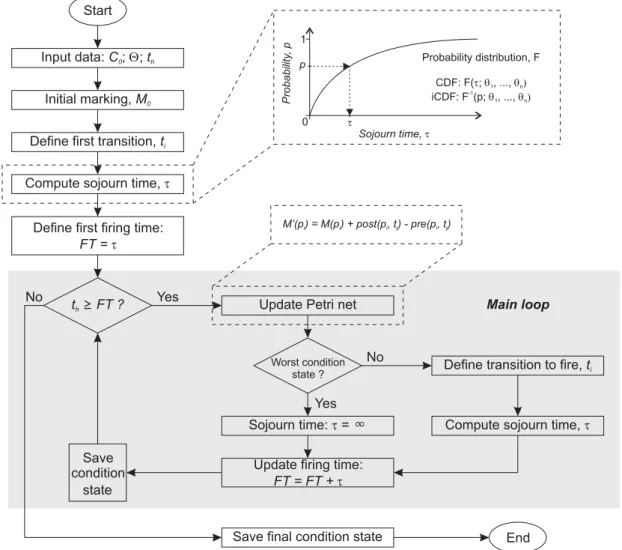
historical data of inspections and maintenance actions to the deterioration model based on concept of timed Petri nets is developed. The sojourn time in each condition level are modelled as probabilistic distributions. The probability distribution that best describes the deterioration process of an infras-tructure is that resulting in higher probabilities of occurrence of the observed transitions. In order to assess what are the parameters of the probability distribution that provides a best fit, the parameters are fitted to historical data through maximum likelihood indicators and optimization algorithms. Fi-nally, in Task 2.4, the most common maintenance strategies are evaluated. The maintenance model is developed based in the Petri net formalism.
WP3 – Evaluation of the maintenance actions impact on performance and cost
Maintenance actions imply direct costs to managing agency and indirect costs to users. User cost are usually associated with limitations of use during the application of maintenance actions. For example, in transportation infrastructures these costs correspond to increased travel time and fuel consumption, as well as, overall dissatisfaction. Agency costs are associated with material and labour costs. The consideration of these costs makes it small-scale maintenance solutions more attractive than correc-tive maintenance actions of greater impact. This approach will also increase the attraccorrec-tiveness of solutions that, although associated with higher costs, result in lower impact on users, like conducting interventions at night or weekend. However, these indirect costs cannot be directly compared to direct cost, since they are allocated to a large number of individuals with little influence in decision-making.
In this work, both direct and indirect costs are considered as two independent impacts. The best maintenance policy is defined as that minimizing both direct and indirect costs or the best balance between them, according to the preferences and financial availability or the decision-maker. This WP, the maintenance model developed in WP2 is applied two different types of infrastructures:
• Task 3.1 – Bridges;
– Task 3.1.1 – Definition of the traffic model;
– Task 3.1.2 – Implementation of the traffic model;
– Task 3.1.3 – Calibration and validation of the traffic model;
• Task 3.2 – Ceramic claddings.
1.4. OUTLINE OF THE DISSERTATION 5
Task 3.1.2, the traffic model will be implemented in software MalLabR. In Task 3.1.3, the traffic will
be tested and the calibration and validation will be performed by comparing the values of the basic traffic parameters (speed, density, and flow rate) obtained through the traffic model implemented and a commercial micro simulation software, Aimsun.
WP4 – Implementation of optimization algorithms in asset management
In this last work package, methods to optimize maintenance policies are defined. This WP can be divided into three tasks:
• Task 4.1 – Definition;
• Task 4.2 – Implementation;
• Task 4.3 – Asset management.
In Task 4.1, the constrains and the objective function of the optimization problem will be defined. Constraints should be set for the acceptable average performance level, as well as the probability of violation of performance thresholds. In terms of costs, it should also be defined objectives in terms of the average values of the direct and indirect costs, but additionally measures to minimize the financial risks should be included, namely minimizing the characteristic cost over the life cycle. In Task 4.2,
the optimization problem will be implemented in software MalLabR using generic algorithms and
evolutionary strategies. Finally, in Task 4.3, the optimization problem is solved considering several objectives of optimization.
1.4
Outline of the dissertation
This dissertation begins with two background chapters, where the state of knowledge regarding Infras-tructure Management System, its main components, and the main numerical techniques that enable them to be modelled are presented. In the following chapters, a description of the deterioration and maintenance model developed is presented and analysis of two case study is described. Finally, the impact of maintenance actions on performance and cost is evaluated as a multi-objective optimization problem.
In this way, the present dissertation is divided into nine chapters, including the present one, as follows:
• Chapter 1: An introduction to the topic is presented, and the main objectives and methodology of the dissertation are identified.
• Chapter 2:A detailed literature review on infrastructure management and maintenance is pro-vided. The chapter begins with definition of an Infrastructure Management System and its main components as an important tool to help managers make informed and optimal decisions based on the analysis of the network data, making reference to several examples of IMS that have been developed over the years. After that, different deterioration models used to predict the future degradation are described and their advantages and limitations are appraised. Special empha-sis is given to Markov chain-based deterioration models and to Petri nets-based deterioration models. In the end, a state of the art on maintenance models is presented.
• Chapter 3: This chapter is dedicated to Petri nets, describing the fundamental concepts and extensions of the Petri nets used in this project.
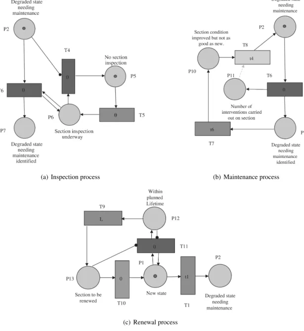
model is presented. After that, the model used to consider maintenance in the system is de-picted. The maintenance model was built from the deterioration model, including inspection, maintenance and renewal processes. In this chapter, the computational framework developed to compute the performance profiles are also described.
• Chapter 5:The deterioration and maintenance models based on Petri net formalism described in Chapter 4 are applied to two bridge components (pre-stressed concrete decks and bearings), using historical data collected by Ascendi. The chapter starts with the validation of the Petri net deterioration model. After that, the Petri net deterioration model is applied to analyse the dete-rioration process over time, and the maintenance model is applied to analyse the consequences of alternative maintenance strategies to control deterioration in bridge components.
• Chapter 6:The deterioration and maintenance models based on Petri net formalism described in Chapter 4 are applied to ceramic claddings. The deterioration model is used to predict the de-terioration of cladding over time and to understand how the different exposure to environmental contribute to degradation. The maintenance model is applied to analyse the consequences of alternative maintenance strategies to control deterioration patters in ceramic claddings. The sample used in this case study is composed by 195 ceramic claddings located in Lisbon, Portu-gal.
• Chapter 7:This chapter focus on evaluate the maintenance impact on performance of a trans-portation network. The concept of resilience was used to quantify the rapidity of rehabilitation of infrastructure and the restoration of traffic flow. The traffic model implemented is based on the macroscopic approach described by Tolba et al. (2005). The calibration and validation of the traffic model was performed by comparing the values of the basic traffic parameters (speed, density, and flow rate) obtained through the traffic model implemented and the commercial micro simulation software, Aimsun.
• Chapter 8: In this chapter, a multi-objective optimization framework based on genetic al-gorithm for asset management of infrastructures is implemented. The optimization finds the maintenance strategies that minimizes maintenance costs, impact of maintenance on users, and maximizes performance indicators. As an example of application, maintenance strategies for the two bridge components analysed in Chapter 5 are optimized. The indirect costs are eval-uated through the traffic model developed in Chapter 7. The case study is part of Portugal’s highway network.