Time-reversal and spatial diversity: issues in a
time-varying geometry test
S.M. Jesus
∗and A.J. Silva
∗∗SiPLAB - FCT, University of Algarve, Campus de Gambelas, 8005-139 Faro, Portugal
Abstract. Underwater acoustic communications in waveguides is known to be prone to severe
multipath, which strongly limits practical transmission rates with actual channel equalization tech-niques. The time reversal principle uses the ocean waveguide response to a basic pulse shape to matched filter the received data sequence. Assuming the ocean response to be a version of the actual pulse shape ocean response corrupted by additive noise, the matched filter output remains a sum of four terms from which only one has the required data sequence in usable form. This paper analysis the ability of such a peculiar matched filter to reject the unwanted terms both with fixed and time-varying source-receiver geometries. One particular parameter with practical interest is the sensitivity of the matched filter performance to a change of the source-receiver range during the processing that induces a mismatch limiting factor. Simulation examples in realistic situations and results obtained with real data, collected during the INTIFANTE’00 sea trial, illustrate the theoretical assertions.
INTRODUCTION
Theoretical developments achieved in various areas of underwater acoustic signal pro-cessing such as time delay estimation, channel equalization and optimization, eventu-ally contributed to the literal explosion of the air-wireless communications in the last 10 years. Conversely, recent developments in air-wireless communications are now becom-ing popular in underwater communications, where it is now frequent to see references to concepts such as digital links, multiple users, local area networks, etc. High-speed data communication requires digital modulation and coherent receivers which, due to the frequency-dependent sound absorption of the ocean channel, are clearly limited. Ef-fective coherent receivers usually exploit spatial diversity and use powerful multichannel equalization algorithms to attain acceptable error rates [1]. Channel equalization is a pro-cess that attempts to undo the channel multipath with a digital filter, which coefficients are adapted on real time according to the variations of the acoustic channel propagation. Due to the high variability of the acoustic channel in practical situations, the usage of test sequences strongly limits the effective throughput of the acoustic link.
A different approach, known as acoustic time-reversal (TR), was originally proposed by [2, 3] and successfully tested at sea in [4]. In digital communications, the application of the TR principle consists in preceding each data packet by a probe signal that is later used as matched-filter to undo the channel multipath for each hydrophone, and then coherently summed over the receiving array channels. This process is known as passive phase conjugation [5, 6] or virtual time-reversal (vTR) [7, 8] and demonstrated with simulated data, in the underwater communication context, in [6, 9] and with real data in [10, 11]. As in acoustic TR, phase conjugation performance will depend upon the
stability of the propagation channel and the ability of the receiving array to correctly sample the most important features of the acoustic field at the useful frequencies.
In practice, there are three main limiting factors in underwater communications: one is the stability of the oceanic characteristics that determine the channel acoustic response; the other is the noise, that can be of environmental nature - sea surface and microstruc-ture induced - or due to electronics; the third, and most important, limiting factor is that due to the experimental geometry, where source and receiver motion relative to the sea surface and bottom are of paramount importance. Of course these limiting factors are not independent among them and often manifest themselves simultaneously. In addition to demonstrating the practical feasibility of TR in the ocean, the experiment by Kuperman
et al., [4] also showed the remarkable temporal stability of this process, since pulses
were successfully refocused up to one week after the original recordings. Through sim-ulations Silva et al. [8], showed that the receiving array does not have to span all the water column or be extremely dense, but must intersect most of the energy propagating in the sound channel. Another important, and an often overlooked problem, is that of the choice of the probe signal window length to be recorded and used at a later time as matched-filter to the incoming data. It was shown in [11] that for each source-receiver range there was an optimal probe signal window length, that minimized the empirical bit error probability.
It is common sense that a major limiting factor in real world applications is source-receiver motion in common tasks such as transmitting telemetry data from untethered measurement instruments and communicating with AUV’s. This paper addresses this problem first from a theoretical point of view, comparing the TR based receiver and the environmental based (MFP) receiver. Then using simulations drawn from an experimen-tal scenario and finally with a real data example.
THEORETICAL BACKGROUND
The baseband matched-filter
In order to introduce the subject let us consider that the system is working in baseband, that the bit sequence {an} is memory less and that the bit rate is such that each pulse is
resolvable, i.e., the pulse duration is larger than the beamwidth of the channel response autocorrelation function. Let us assume that the transmitted signal is Pulse Amplitude Modulated (PAM) and can be written as
s(t) =
+∞
∑
n=−∞
anp(t − nTb), (1)
where anis the symbol sequence, assumed white with power σa2, Tbis the symbol period
and p(t) is the pulse shape function. Assuming the acoustic channel as a linear time-invariant system with impulse response g(t, θ ), the received signal is
where w(t) is an additive zero mean white Gaussian noise with power σw2, assumed to be uncorrelated with the signal and from sensor to sensor and where θ is a vector containing the environmental and model parameters, denoting the dependence of the channel response on the environment. In order to simplify the notation let us consider the discrete version of (2)
y(θ ) = G(θ )s + w (3)
= x(θ ) + w, (4)
where the observation vector yT(θ ) = [y(0, θ ), y(1, θ ), . . . , y(N − 1, θ )], is obtained over
a set of N temporal samples at a sampling rate Ts≤ 1/2 fmax, where fmaxis the maximum
frequency in the observed signal y(t). Considering that the channel impulse response and the signal s, of dimension M × 1, as causal signals, the matrix G(θ ), with dimension
N × M, is lower triangular with discrete and delayed replicas g(θ ) of the channel
response g(t, θ ), conditioned in the vector parameter θ . Using this notation and with the hypothesis stated above, both the noise and the observation will be additive white Gaussian distributed such that w :N [0,σw2I] and y :N [G(θ)s,σw2I].
The problem can be cast as the detection of signal s(t), conditioned on the channel response g(t) and on the parameter vector θ . This is a classical problem, which solution is given by the Neyman-Pearson (NP) theorem when the noise is Gaussian and by the (matched-)filter that maximizes the signal-to-noise ratio (SNR) at its output, in the general case. The matched filter in this case is given by
h(n, θ ) = h0x(n0− n, θ ), (5)
where h0 and n0 are an arbitrary amplitude factor and a constant delay, respectively.
The optimality of the matched-filter is attained when n0= N − 1 and the matched-filter
output is sampled at n = N − 1, the duration of the observation record. The convolution of the observation y with filter (5) gives
z(n, θ ) = hTn(θ )y(θ ) = zo(n, θ ) + wo(n), (6)
where
hn(θ ) = h0G(θ )s|n, (7)
and where |n index denotes a delay of n samples. Replacing (3) in (6) gives the signal
and the noise terms as zo(n, θ ) = hTn(θ )G(θ )s and wo= hTn(θ )w, respectively. The SNR
at the output of the matched-filter can now be defined as
ρ (n, θ ) =|zo(n, θ )|
2
E[w2
o(n)]
. (8)
Replacing the values of z0(n, θ ) and wo(n) into the SNR expression gives
ρ (n, θ ) = s
TGT(θ )h
n(θ )hTn(θ )G(θ )s
σw2hTn(θ )hn(θ )
which maximum value is
ρmax(θ ) =
sTGT(θ )G(θ )s
σw2 , (10)
obtained when the filter takes the form (7) and n = N −1. Despite the apparent simplicity, the matched-filter concept is not always easy to implement in practice. This is due to the difficulties associated with (7) which, in the underwater communications context, deal with the fact that the channel response G(θ ) is unknown. Besides the classic solution of adaptive equalization, there at least three other possibilities used in practice:
• one is to ignore the channel response and use a receiving filter simply matched to emitted signal, such that hn= h0s. This plain matched filter is commonly used in
active sonar where the emitted signal is known and on classic underwater commu-nication systems, where the receiving filter is only given by the pulse shape p(t) as used on the signal coding expression (1).
• a second case became popular with the increasing usage of matched-field process-ing (MFP) techniques in the 80’s, where the incomprocess-ing signal is matched with a model-based replica ˆg( ˆθ ) of the channel response g(θ ) whenever a sufficiently
ac-curate approximation of the model parameter vector ˆθ of the true parameter vector θ is available. In that case an estimate ˆhn( ˆθ ) = h0G( ˆˆ θ )s|nis used, instead of hn(θ ).
• the third situation arose more recently, with the appearance of the so-called time-reversal (TR) techniques that use the recording of the channel response to a single pulse shape (probe signal) during a given interval that is then used as matched-filter for the incoming signal at a later stage. This technique requires two important assumptions: one is that the source is cooperant with the receiver so it can, at regular intervals, transmit a channel probe so it can be used to calibrate the matched filter at the receiver and two, that in the time interval between probe signals the acoustic channel is sufficiently stable so the last probe, recorded a few seconds (or minutes!) before, can be used as the actual channel response, as required by the optimum receiver (7). Another important difference is that the recorded probe signal, apart from the signal itself, also contains noise which is implicitly used in the matched filter with, so far, unpredictable results.
Matched-filter relative performance
Leaving aside the case of the plain matched-filter where the channel response is ignored, it is interesting to perform a comparison between the MFP version of the matched-filter and its TR counter part. This comparison can be easily made using the matched-filter output SNR, since the SNR is a monotonic function of the probability of detection. Let us first consider the MFP case where the receiving filter is given by
conditioned on the acoustic model response ˆg and the assumed model environmental parameter vector ˆθ . Replacing (11) as h(θ ) into SNR expression (9), allows to write
ρMFP(n, θ ) =
|sTGT(θ ) ˆG( ˆθ )s|2
σw2k ˆG( ˆθ )sk2
. (12)
The maximum SNR performance of the MFP matched filter is obtained when ˆG( ˆθ ) =
G(θ ) and n = N − 1, i.e., when the parameter vector and the channel response are
perfectly modeled and the matched filter peak response is correctly chosen, such that
ρMFP−max=
kG(θ )sk2
σw2 . (13)
In the TR case the matched-filter is given by
h0n(θ ) = G0(θ )s + w0 (14)
where0denotes that the recording was made at a previous time such that the filter output can be written as1
z = [G0s + w0]T[Gs + w] (15)
= sTG0TGs + sTG0Tw + w0TGs + w0Tw, (16)
where in the four terms obtained in (16), the first term corresponds to the desired signal, while the other three are noise components and treated as such in the evaluation of the output SNR. Thus, using definition (8), the output SNR is the ratio between the square module of the first term divided by the expectation of the square of the sum of the three last terms. Assuming that the noise is white and thus decorrelated between the time when the probe is recorded and when the actual matched-filtering takes place, greatly simplifies the final output SNR expression that can be written as
ρTR=
|sTGTG0s|2
σw2sT[G0TG0+ GTG]s
. (17)
This is a curious expression that shows an upper term that depends on the correlation of the channel responses at the probe time and at the actual receiving time, and a lower term that is the direct summation of the auto channel responses to the noise part. Due to the particular form of this filter an upper bound on its performance can not be obtained analytically. It is however interesting to perform a comparison between the two matched-filters making the ratio between (17) and (12) to obtain
ΛTR/MFP=
k ˆG( ˆθ )sk2|sTGTG0s|2
|sTGT(θ ) ˆG( ˆθ )s|2sT[G0TG0+ GTG]s, (18)
1to simplify the notation the dependency on time index n and on the vector parameter θ will be omitted
where it can be easily remarked that if the same error is made in the TR than in the MFP, then ˆG = G0 and the performance ratio ΛTR/MFP is always ≤ 1, while in the no error case, ˆG = G0= G, we have thatΛTR/MFP= 0.5. In other terms, this means that if the
same environmental mismatch exists in the two implementations, the TR approach will have a poorer performance than the MFP based approach, which is possibly explained by the fact that in the TR approach there is a re injection of noise in the filter. Of course the question is how “close” can the model-based channel response be from the true channel response or equivalently how much can the channel response change in a given time interval between the probe signal and the actual message. The TR approach became popular with the experimental evidence that the acoustic channel was very stable relative to matched filtering a whole array of sensors in a shallow water environment [4]. There are however two aspects not covered by that experimental conclusions that are of major importance in practical underwater acoustic communications: one is the frequency band at which the experiment was performed, was significantly lower that that used in useful underwater communications systems, and the other is that both source and array where static in the water so no significant geometrical mismatch existed. An analysis of the relative performance of the two detectors in a realistic situation of a time-varying geometry environment encountered during the INTIFANTE’00 sea trial is accomplished via simulation in the next section.
SIMULATION AND REAL DATA RESULTS
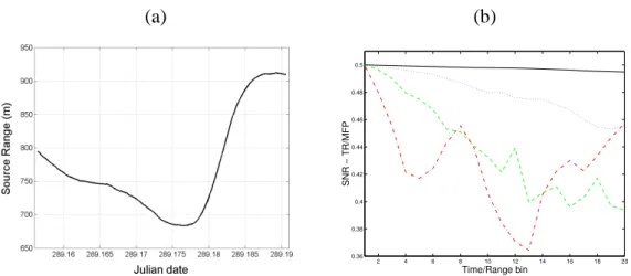
This section gives a simulated example drawn from Event I of the INTIFANTE’00 sea trial that took place in the continental platform off the town of Setúbal (Portugal) in October 2000. This event involved an acoustic source suspended from a free drifting research vessel transmitting acoustic signals to a moored 16-hydrophone receiving ver-tical line array (VLA). The source was at 70 m depth, steaming away from the VLA and making stations at various ranges. The environment was characterized by a nearly range independent 120 m-depth shallow water waveguide with a slightly downward re-fracting sound speed profile and a sandy bottom with 1750 m/s sound speed, a density of 1.9 g/cm3and a compressional attenuation of 0.8 dB/λ . The transmitted signals were Differential Phase Shift Keying (DPSK) modulated sequences with a center frequency of 1.6 kHz and bandwidths between 100 and 350 Hz. The simulation was performed in the frequency domain using 5 frequencies equispaced in the band 1450 to 1750 Hz. A channel probe signal was transmitted at regular intervals of 20 seconds in between the data signals. In order to test the relative performance of the matched-filters against time-geometry, the ratio Λ of equation (18) was estimated with ˆG = G0and where the mismatch with G was due only to range variations during source drift. Realistic values of source drift were estimated during station 1 using data shown in figure 1(a). Figure 1(b) shows the results ofΛfor one data window of 20 seconds for drift speeds of 0.02, 0.1, 0.3 and 1 m/s. It can be easily seen that, as expected, the relative performance of the two implementations starts at 0.5 and significantly decreases during the time/range window, depending on the drift speed: generally an higher drift speed means a larger performance drop and more variable behavior. The variations of performance are related
(a) (b) 2 4 6 8 10 12 14 16 18 20 0.36 0.38 0.4 0.42 0.44 0.46 0.48 0.5 SNR − TR/MFP Time/Range bin
FIGURE 1. source-receiver range variation during station 1 of Event 1 (a) andΛratio (18) (b): 0.02 m/s (solid), 0.1 m/s(dot), 0.3 m/s (dash) and 1 m/s (dash-dot).
to the range variation relative to the signal mean wavelength (∼1 m in this case). In
or-0 2 4 6 8 10 12 14 16 18 20 0 0.1 0.2 0.3 0.4 0.5 0.6 0.7 Error probability reduced time [s]
FIGURE 2. empirical probability of error during 20 seconds time window.
der to illustrate the same effect with real data, figure 2 shows the empirical probability of error estimated during a time window of 20 seconds on station 4 of Event 1, where the previous probe signal was used to matched filter the data prior to summation over the VLA hydrophones. It can be noticed that, in agreement with the expectations drawn from the simulation, the error probability strongly varies during the 20 s data window.
CONCLUSIONS
Unlike its airborne counterpart, underwater communications suffers from an extremely harsh propagation environment due to anisotropy, sound absorption and refraction. In shallow water the problem is particularly severe due to multiple reflections on the ocean
bottom and surface, making it difficult to obtain a transmission rate of a few kbauds at ranges of several water depths. In any communication system the main component dealing with channel distortion is the receiving filter. Traditionally, the receiving filter is composed of a replica of the emitted pulse shape followed by a channel equalizer. This paper presents a theoretical comparison of two alternatives for the receiving filter: the time-reversal (TR) approach, that matched-filter the data with the channel response at a previous time, and the model-based MFP approach, that attempts to numerically compute the channel response from a priori environmental information. It is shown that, for the same channel distortion, the MFP based technique always outperforms (in terms of output SNR) the TR approach. Simulations drawn from a realistic example where channel mismatch is uniquely due to a drifting source-receiver geometry, confirm the theoretical assertions. An example obtained from the INTIFANTE’00 data set show an empirical bit error probability with a similar behavior to that seen in the simulations.
ACKNOWLEDGMENTS
The authors would like to thank the support of the NATO Undersea Research Centre and the Instituto Hidrográfico during the INTIFANTE’00 sea trial. This work was also partially supported by FUP/Ministry of Defence under project LOCAPASS, by the AOB - REA Joint Research Project and the HFi - High Frequency Initiative.
REFERENCES
1. Stojanovic, M., Catipovic, J., and Proakis, J., J. Acoust. Soc. Am., 94, 1621–1631 (1993). 2. Jackson, R., and Dowling, R., J. Acoust. Soc. Am., 89, 171–181 (1991).
3. Dowling, R., and Jackson, R., J. Acoust. Soc. Am., 91, 3257–3277 (1992).
4. Kuperman, W., Hodgkiss, W., Song, H. C., Akal, T., Ferla, C., and Jackson, D., J. Acoust. Soc. Am.,
103, 25–40 (1998).
5. Dowling, R., J. Acoust. Soc. America, 95, 1450–1458 (1994).
6. Rouseff, D., Fox, L., Jackson, D., and Jones, D., “Underwater Acoustic Communications Using Passive Phase Conjugation,” in Proc. of the MTS/IEEE Oceans 2001, Honolulu, Hawai, USA, 2001, pp. 2227–2230.
7. Gomes, J., and Barroso, V., “A Matched Field Processing Approach to Underwater Acoustic Com-munication,” in Proc. of the MTS/IEEE Oceans 1999, Seattle, USA, 1999, pp. 991–995.
8. Silva, A., Jesus, S., Gomes, J., and Barroso, V., “Underwater Acoustic Communications Using a “virtual” Electronic Time-Reversal Mirror Approach,” in 5th European Conference on Underwater
Acoustics, edited by P. Chevret and M.Zakharia, Lyon, France, June, 2000, pp. 531–536.
9. Edelmann, G., Hodgkiss, W., Kim, S., Kuperman, W., Song., H., and Akal, T., “Underwater Acoustic Communications Using time-reversal,” in Proc. of the MTS/IEEE Oceans 2001, Honolulu, Hawai, USA, 2001, pp. 2231–2235.
10. Jesus, S., and Silva, A., “Virtual Time Reversal in Underwater Acoustic Communications: Results on the INTIFANTE’00 Sea Trial,” in Proc. of Forum Acusticum, Sevilla, Spain, 2002.
11. Silva, A., and Jesus, S., “Underwater Communications Using Virtual Time-Reversal in a Variable Geometry Channel,” in Proc. MTS/IEEE Oceans’2002, Biloxi, USA, November, 2002, pp. 2416– 2421.