ABSTRACT: The wind energy research has grown substantially in the past few years, considerably fostered by the pursuit for a clean and sustainable energy source. Improvements on the design methods are increasingly needed. The purpose of this research is to investigate the use of the Loewy´s lift deiciency function (LDF), also named Returning Wake Model, coupled with a non-stationary Blade Element-Momentum Method (BEM). The LDF simulates the inluence of the wake behind the wind turbine on its capacity to generate power. It is expected that this model reduce the dependency of the several empirical parameters necessary in other wake models which are currently used. Aiming to validate the results obtained in this new approach they are compared with those provided by commercial computational software and they have proven to be very consistent. It is concluded that the method is feasible to be used as an eficient design and optimization tool of upwind horizontal axis wind turbine blades.
KEYWORDS: Blade element method, Loewy´s lift deiciency function, Non stationary BEM, Wind turbine, Wind turbine blade design, Returning wake model.
Unsteady Blade Element-Momentum Method
Including Returning Wake Effects
Cláudio Tavares Silva1,2, Maurício Vicente Donadon1
INTRODUCTION
Wind turbines operate in a hostile environment in which strong low luctuations, mainly due to the nature of the wind, can produce high and variable loads on its components. hese loads, combined with the elastic behavior of the turbine structural components, compromise the overall energy generation eiciency and cannot be neglected during the design phase. he need for experimental and computational approaches to investigate the behavior of unsteady loads produced on a wind turbine blade has grown in proportion to the growing nominal power and size of the actual horizontal axis wind turbines.
he objective of this work is to evaluate the mathematical model of the Loewy´s lit deiciency function (LDF) to be included in a computational package enabling the optimal design of horizontal axis wind turbine blades. his model allows the inclusion of non-stationarities as well as an approximation of the efects of the downwind wake dynamics on turbine aerodynamic performance. his inclusion of non-stationarities and the efects of the downwind wake allow more realistic results for the aerodynamic loads than the simple Blade Element-Momentum (BEM) method, and consequently leads to better designs of structural components.
he overwhelming majority of computer packages and procedures actually use semi-empirical models to represent the inluence of the wake in the overall aerodynamic performance of a wind turbine blade. he LDF (Loewy, 1957) is an analytical solution based on the classical heodorsen theory (heodorsen, 1935). he use of an analytical model reduces the dependence on experimental tests for the adjustment of empirical parameters needed to calibrate
1.Instituto Tecnológico de Aeronáutica – São José dos Campos/SP – Brazil 2.Universidade Tecnológica Federal do Paraná – Curitiba/PR – Brazil
Author for correspondence: Cláudio Tavares Silva | Praça Marechal Eduardo Gomes, 50 – Vila das Acácias | CEP 12228-900 São José dos Campos/SP – Brazil |
E-mail: ctavares@ita.br
these semi-empirical engineering models. Furthermore, an analytical resolution results in a more elegant mathematical solution, computationally feasible and suiciently fast to provide blade design optimization.
he induced efects generated by the shed wake have been modeled using two general approaches: dynamic inlow methods and vortex wake methods.
he principles of the dynamic inlow approach are attributed to Carpenter and Freidovich (1953). he idea is to consider the unsteady aerodynamic lag of the inlow development over the rotor disk in response to changes in blade pitch inputs of changes in rotor thrust. hey are written in the form of ordinary diferential equations, with a time constant (or constants) representing the dynamic lag in the build-up of the inlow. One of its less satisfying aspects is that time constants must be obtained by experimental calibrations.
Vortex wake models are based on the assumption of an incompressible potential low, with all vorticity being assumed concentrated within vortex ilaments (which in the case of rotors require a coupling to the blade lit distribution). he induced velocity ield can be determined through the application of the Biot-Savart low. Diferent approaches are encompassed ranging from prescribed to free vortex techniques. he prescribed wake models are strictly applicable when the operating conditions are nominally steady-state, i.e., in a steady wind. he free vortex methods have fewer potential limitations. hey have been widely developed to be used in helicopters rotor analyses. Free vortex methods are based on discretized, inite-diference representation of the governing equations for the wake, and when solved, they track the evolution of discrete vortex elements through the low. he number of discrete elements per vortex ilaments can be very large, making the tracking process memory intensive and computationally demanding.
Leishman (2002) presents more details about dynamic inlow models and vortex wake models.
THEORY AND METHODS
THE CLASSICAL BLADE ELEMENT MOMENTUM METHOD
The BEM method presented by Glauert (1935) enables to calculate the steady loads and also the thrust and power
using different settings on wind speed, rotational speed and pitch angle. The method couples the momentum theory with local events taking place at the actual blades. The blade is analyzed as a number of independent stream tubes. In each one, the induced velocity is calculated by performing the conservation of momentum, and the aerodynamic forces are found with the 2D aerodynamic theory and airfoil data. The stream tubes are discretized into N annular elements. The lateral boundary of the elements does not admit any flow across them. Some assumptions are made for the annular elements: no radial dependence, that is, one element cannot be affected by the others; the forces from the blade on the flow are constant in each annular element, corresponding to a rotor with a number of blades.
A correction known as Prandtl´s tip loss factor (Glauert, 1935) is introduced to correct this latter assumption in order to compute a rotor with a finite number or blades.
A relative velocity Vrel seen by a blade section is a combination of axial velocity V0(1–a), in which a is the
axial induction factor, and the tangential velocity (1–a') ϖr, where a' is the radial induction factor at the rotor plane (Fig. 1). The angle θ is the local pitch angle of the blade element, i.e., the local angle between the chord and the plane of rotation. It is a combination of the pitch angle, measured between the tip chord, the rotor plane and the twist of the blade, relative to the tip chord. ϕ is the flow angle, measured between the plane of rotation and the relative velocity. The local angle of attack α is obviously found.
Figure 1. Velocities at rotor plane.
rel
V
(
)
0 1
V a
(
1)
r +a
P rb
r
x2
y2 y3
3 y4
z z
z
2 x3
x4
4
tilt
cone
rt rs
The algorithm for the BEM model can be summarized as the sequence of steps that follows. Since different control volumes are assumed to be independent, each blade element can be treated separately and the solution at one radius can be computed before solving another radius. The following algorithm is applied for each control volume.
Step (1): Initialize a' (axial induction factor) and á (radial induction factor), typically a = a' = 0.
Step (2): Compute the low angle ϕ.
Step (3): Compute the local angle of attack α.
Step (4): Read of the lit Cl(α) and drag Cd(α) coeicients from a table.
Step (5): Compute Cn and Ct, respectively normal and tangential aerodynamic force coeicients.
Step (6): Recalculate a and a'.
Step (7): If a and a' have changed more than a tolerable amount, repeat step (2), or else inish.
Step (8): Compute local loads on the blade element. All equations necessary to perform the above algorithm can are described by Burton (2001) and Hansen (2007).
UNSTEADY BEM MODEL
In order to obtain good estimates of the annual energy production of a wind turbine, a steady BEM method is adequate to compute the steady power curve. But in reality the rotor of a wind turbine feels the inherent unsteadiness of the wind caused by atmospheric turbulence, wind shear and the presence of the tower. It is necessary to use an unsteady BEM method to compute realistically this variable behavior of the wind.
One simple model and additional coordinate systems can by placed at the wind turbine and its blades so it is possible to know the relative position of any blade element at any time. his simple model is depicted at Fig. 2.
An inertial system of coordinates is placed at tower base and named System 1. System 2 is non-rotating and fixed in the nacelle. System 3 is solidary to the shaft turbine and rotates with it, and system 4 is aligned with one of the blades. The tilt and cone angles are shown and the azimuthal position of the blade is set by de wing angle
θwing, not depicted.
he undisturbed wind velocity seen by the blade is found by a simple coordinate transformation clearly detailed by Hansen (2007).
Figure 2. Coordinate systems.
he essence of the BEM method is to determine the induced velocity and thus the local angle of attack. his is achieved by a summation of vectors, Vrel = V0+ Vrot+W, all
written at the element blade coordinate system (System 4, Fig. 3), in which the induction velocity is the term W.
With the induced velocity known, the low angle and angle of attack are found.
(
)
, ,
tan rel z
p rel y
V V
ϕ= α ϕ= − β θ+
- (1)
forward light (similar to the result of the liting line for an elliptically loaded circular wing) is:
(
)
0 2 n T W A ρ = ⋅ = + ⋅ n WV n n W (2)
in which n is the unit vector in the direction of the thrust, which in System 3 has the coordinates n=[0,0,1]T.
It is assumed that only the lit contributes to the induced velocity, and that the induced velocity acts in the opposite direction to the lit. he force from this blade at radial position is assumed to afect the air in the area
dA = 2πrdr/B, so that all B blades cover the entire annulus of the rotor disc at radius r.
he following expression can be derived for one blade, according to Hansen (2007),
(
)
0(
)
0
cos cos
2 4
2
n z
L dr BL
W W rdr rF F B ϕ ϕ π πρ ρ − − = = + ⋅
+ ⋅ V n n W
V n n W (3)
For the tangential component a similar expression is postulated,
(
)
0 sin 4 t y BL W W rF ϕ πρ − = = + ⋅V n n W (4)
in which F is Prandtl’s tip loss factor.
If the rotor is yawed (and/or tilted), there will be an azimuthal variation of the induced velocity, so that it is lower when the blade is pointing upstream in relation to when the same blade, half a revolution later, is pointing downstream. The physical explanation for it is that a
blade pointing downstream is deeper into the wake than a blade pointing upstream. This means that an upstream blade sees a higher wind speed and thus produces higher loads than the downstream blade, which produces a beneficial yawing moment that will try to turn the rotor more into the wind, thus enhancing yaw stability. The yaw model describes the distribution of the induced velocity. If a yaw model is not included, the BEM method will not be able to predict the restoring yaw moment, according to Hansen (2007):
(
0)
0 1 tan cos
2 wing
r R
χ θ θ ⎞
⎛ ⎛ ⎞
= ⎜ + ⎜ ⎟ − ⎟
⎝ ⎠ ⎠
⎝
W W (5)
in which the wake skew angle, X, is deined as the angle between the wind velocity in the wake and the rotational axis of the rotor.θ0 is the angle in which the blade is deepest into the wake. he skew angle can be found as:
(
0)
0
cosX= ⋅ + + n V W
n V W
(6)
he skew angle is assumed to be constant with the radius and can be computed at a radial position close to r/R = 0.7.
The induced velocity is now known at the new azimuthal position at time t+∆t, θwing(t+ ∆t)= θwing(t)+ ω∆t. The angle of attack can thus be evaluated from the equation and the lift and drag coefficients can be looked up from a table. The normal, pz, and tangential, py, loads can be determined from:
cos sin y sin cos
z
p =L φ+D φ p =L φ−D φ (7)
in which
2 2
1 1
2 rel l 2 rel d
L= ρV cC D= ρV cC (8)
he algorithm can be resumed like the following:
Step (1): Initialize all necessary data (geometry and run parameters);
Step (2): Initialize the position and velocity of blades; Step (3): Discretize the blades into N elements; Step (4): Initialize the induced velocity;
- for n=1 to max time step (t=n∆t)
- for each blade
- for each element 1 to N
Step (5): Compute relative velocity to the blade element using old values for induced velocity;
Step (6): Calculate low angle and thus the angle of attack (Eq. 1);
Step (7): Determine static drag and lit coeicients from tables;
Step (8): Compute lit and drag for each blade element (Eq. 8);
Step (9): Compute loads (Eq. 7);
Step (10): Compute new equilibrium values for induced velocities (Eqs. 3 and 4);
Step (11) Calculate the azimuthal variation from Eq. 5 and compute the induced velocity for each blade;
Step (12): Compute momentum, thrust and power; Step (13): Increment time step and repeat from step (5). he equations of the BEM method must be solved iteratively. he low angle and thus the angle of attack depend on induced velocity. But the described algorithm is unsteady, therefore time is used as relaxation. Ater blades have moved in one time step an azimuthal angle of ∆θwing=ω∆t (for small ∆t´s), values from the previous time step are used on the right hand side of equations for W when updating new values for induced velocity. his can be taken into account since induced velocity changes relatively slowly in time. his eliminates the need of calculating the induction factors and use of tolerance.
DETERMINISTIC WIND MODEL
he exponential model used to simulate wind shear. It controls the wind speed according to the altitude, and the shear parameter used is 0.2. Detailed information about this wind shear model was described by Hansen (2007).
The wind is also influenced by the presence of the tower. The simple model used to simulate the tower shadow assumes potential flow. All details about this simple model were also described by Hansen (2007). This model is a bad approximation for a downwind machine, in which each blade passes the tower wake once every revolution. However, for an upwind machine, the object of this study, the model provides good estimation. Also, the turbulent part of the real atmospheric wind should be added for a realistic time simulation for a wind turbine. For this initial investigation no atmospheric turbulence is added to the simulation.
LOEWY´S LIFT DEFICIENCY FUNCTION
The problem of calculating the aerodynamic loading on an oscillating profile was first approached by Glauert (1929), but it was only properly solved by Theodorsen (1935). Theodorsen’s approach gives the solution for unsteady aerodynamic loading on a 2D oscillating airfoil in an inviscid and incompressible flow, and subject to the assumption of small disturbances. Theodorsen’s problem is to obtain the solution for loading on the surface of the airfoil under the condition of forced harmonic oscillations.
For a simple harmonic motion of the airfoil the solution given by heodorsen in a way that represents a transfer function relating the forcing input (angle of attack) and the aerodynamic response (pressure distribution, lit, and pitching moment). he approach is summarized by Bisplinghof et al. (1955). See also Bramwell et al. (1976) and Johnson (1980) for a detailed exposition of the theory.
heodorsen’s theory is not suitable for studies involving rotors. In these types of problems sections of blades can ind wake vorticity due to other rotor blades, as well as the returning wake from the blade in question. his fact was recognized by Loewy (1957) and Jones (1958). hey built a two-dimensional model of a 2-D blade section with a returning shed wake, as shown in Fig. 4.
As in heodorsen’s model, the shed wake is modeled with 2-D lat surfaces of vortices, but now with a series of surfaces below the airfoil section with a vertical separation h, which depends on the speed induced by the rotor disc V and the number of blades Nb. Loewy shows that, in this case, the lit on the blade can be expressed by replacing the function heodorsen by the named Loewy’s function.
(
)
( )
( )( )( )
( )
(
( )
( )
( )
)
2
1 1
2 2
1 0 1 0
2
, ,
2
H k J k W
C k h
H k iH k J k iJ k W
ω Ω + ʹ = + + + (9)
in which it is known for Loewy’s function of Loewy’s lit deiciency function.
For a rotor with Nb blades the complex function W is written as:
Δψ ω Ω
(
)
( ) 1 2 1 , , , i b i e kh N b b khW b N e e
The wake spacing ratio h/b can be determined from the spacing of vortex sheets that are laid down below the rotor. If an average induced velocity vi=λΩR is assumed, then during a single rotor revolution the shed wake generated by a single blade will be at a distance h=(2π/Ω)vi below the rotor. For a multiple blade rotor the spacing is (2π)vi/ ΩNb, i.e.
2 4
b
h R
b N b
λΩ π λ
Ω σ
= = (11)
in which σ is the rotor solidity.
Representative results from Loewy’s theory show that the main consequence of including shed vorticity below the blade is that it serves to amplify or attenuate the unsteady lift response, depending on the reduced frequency, wake spacing and wake phase. The most important effects are for lower reduced frequencies, with oscillations at the harmonics of the rotor rotational frequency (Leishman, 2000).
Several aspects related to the non-stationarity of the operating environment of a wind turbine need to be addressed during its project. Among them there are the main variations in wind speed (gust and wind shear),
dynamic inflow, yaw and tower shadow, turbulence, wake dynamics and interactions blade/wake, and the dynamic stall. The adoption of a non-stationary BEM method using a dynamic inflow model is a solution that tends to enhance the results, proving to be a good option to introduce the study of non-stationarity in the design of a wind turbine blade. However the same problems related to the physics of the method remain.
Unsatisfactory aspects of the inflow theory are the so-called dynamic time constants employed in the methods. They are developed using the concept of apparent mass and inertia of the fluid surrounding the rotor (noncirculatory effect) as opposed to the delay of the dynamic evolution of wake vortices (circulatory effects). The concept of apparent mass applied to the rotor also assumes equivalence between the apparent force of the rotor disk accelerating in a stopped fluid and the force in a fluid accelerating through a permeable actuator disc, which certainly is not an accurate analogy.
Loewy proposes a solution to the problem of aerodynamics of rotors affected by non-stationarity generated by shed wake. It is based on Theodorsen’s solution applying a suitable physical model for Figure 4. Loewy’s returning wake problem (Leishman, 2000).
C
C C
C C C
C C
C C
C C
∆ψ γb
γb γ
w = 0
n=0, m=0
n=1, m=0
h
h 4λ
m=1
m=2
m=1
m=2
m=1
m=2
n=2, m=0
x,ζ
∞ ∞
α=θ
=
V
iωt
rotorcraft aerodynamics. The results obtained in the solution of problems related to helicopter hovers, and duly validated with experimental results, confirm the efficiency of the method.
he aerodynamics of a helicopter hover resembles in many aspects the aerodynamics of the blades of a wind generator. his similarity, coupled with the need for a mathematical model for the wind generator blade design that considers the conditions of non-stationarity of the phenomena involved in its aerodynamics, are the main motivators for this work.
he corrections using Loewy’s model are applied for the Equation 2.8 in order to provide the lit deiciency described above. he corrected equations can be rewritten. No corrections are applied to the drag force.
2
1
2 rel l
L= ρV cC C (12)
VERIFICATION AGAINST AN INDUSTRY-STANDARD SOFTWARE
The commercial package used for result validation is the GH Bladed V4.1, distributed by GL Garrad Hassan (2012), an independent renewable energy consultancy. GH Bladed is an industry-standard integrated software package for the design and certification of onshore and offshore turbines. It provides user with a design tool that has been extensively validated against measured data from a wide range of turbines and enables the conduction of the full range of performance and loading calculations (Garrad Hassan & Partners, 2011).
Its manual postulates that GH Bladed uses the same methods employed at the present work. hat is, combined blade element and momentum theory, wake rotation with radial induction, tip and hub loss models, which is suppressed for the present comparison, dynamic wake model and dynamic stall, also suppressed.
An educational version of de GH Bladed GH Bladed 4.1, with a limitation of 10 blade elements, is used.
he object of study is a 2MW wind turbine. he main used parameters and data are shown in Tables 1 and 2.
All necessary data, like angle of attack, lit, drag and moment coeicients are described by McGee and Beasley (1976).
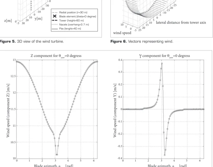
Just for visualization, BEM NE has a graphical interface that shows a simpliied illustration of the wind turbine and his main geometrical parameter. his is shown at Fig. 5.
The developed computational routine uses these same data to be compared with the results of both packages. It also uses de same model for wind shear, i.e., the exponential Table 2. Blade geometry.
Distance along
blade (m) Chord (m)
Aerodynamic twist (deg)
Aerofoil section
0 2.07 0 cylinder
1.15 2.07 0 cylinder
3.44 2.76 9 cylinder
5.74 3.44 13 NASA
LS(1)-0421
9.19 3.44 11 NASA
LS(1)-0421
16.07 2.76 7.8 NASA
LS(1)-0421
26.41 1.84 3.3 NASA
LS(1)-0417
35.59 1.15 0.3 NASA
LS(1)-0413
38.23 0.69 2.75 NASA
LS(1)-0413
38.75 0.03 4 NASA
LS(1)-0413
Table 1. General characteristics of rotor and turbine.
Rotor diameter 80 m
Number of blades 3
Hub height 61.5 m
Tower height 60 m
Tilt angle of rotor to horizontal 4 deg
Cone angle of rotor 0 deg
Blade set angle 0 deg
Rotor overhang 3.7 m
Rotational sense of rotor, viewed from
upwind Clockwise
Position of rotor relative to tower Upwind
Aerodynamic control surfaces Pitch
Radial position of root station 1.25 m
Cut in windspeed 4 m/s
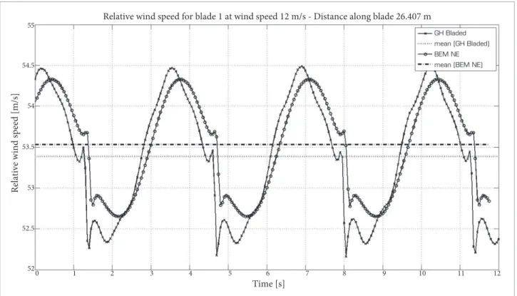
Figure 7. Wind speed components.
Z component for θyaw=0 degress
γ
component for θyaw=0 degressWind speed (component Z) [m/s] Wind speed (component Y) [m/s]
Blade azimuth,θwing[rad] Blade azimuth,θwing[rad]
0 1 2 3 4 5 6 0 1 2 3 4 5 6
13 0.4
0.3
0.2
0.1
0
-0.1
-0.2
-0.3
-0.4 12.5
12
11.5
10.5
10 11
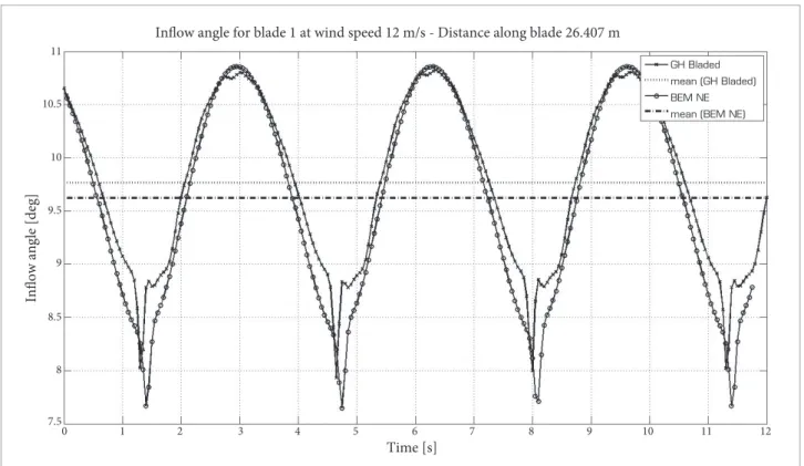
Figure 6. Vectors representing wind. Wind spedd vectors for θyaw=0 degress
ground height
lateral distance from tower axis
wind speed
85 80 75 70 65 60 55 50 45 40 35
-20-25 -15 -5 5 15 25 5 10
-10
0
0 10 20 -5
x[m]
Wind turbine 3D view - yaw=0º, tilt=-4, wing=0º, cone=0º
Radial position (r=30 m) Blade element (theta=0 degree) Tower (height=60 m) Nacele (overhang=3.7 m) Pás (lenght=40 m)
z[m] y[m]
100 90 80 70 60 50 40 30 20 10 0 -30 -20 -10 0 10 20 30 -5 0
Figure 5. 3D view of the wind turbine.
vertical shear model with wind shear coefficient 0.2 and the potential flow model for the tower shadow. Details about the models for wind shear end tower shadow were described by Hansen (2007).
Figure 8. Shaft Power (a) and Pitch angle (b) control map.
(b)
Hub wind speed [m/s]
Bladed Educational - Licensed to: Instituto
Tecnológico de Aeronáutica
4 6 8 10 12 14 16 18 20 22 24 26 2.2
2.0 1.8 1.6 1.4 1.2 1.0 0.8 0.6 0.4 0.2 0.0
Shaft power [MW]
Hub wind speed [m/s]
Bladed Educational - Licensed to: Instituto
Tecnológico de Aeronáutica
4 6 8 10 12 14 16 18 20 22 24 26 2.2
20
15
10
5
0
-5
Pitch angle [deg]
(a)
RESULTS AND DISCUSSION
he most important aerodynamic and performance results are shown and compared here. It is important to mention that the GH Bladed package has a pitch control module that changes the pitch angle of the blades in each time step according to the wind speed, rotor speed and output power. he developed computational routine, named here BEM NE, uses this same pitch angle control map in order to achieve the correct level of the shat power, once it does not have a control module. his control map is depicted in Fig. 8b as also the shat power (Fig. 8a) against diferent wind speeds.
he blades of the wind turbine used in this study are designed to produce 2MW power between wind speeds of 12 and 25 m/s, at the rotor speed 18 rpm. Results at 12 and 18 m/s wind speed are compared.
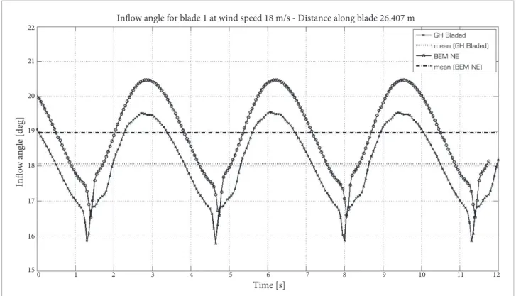
At irst the results obtained for 12 m/s wind speed is shown. Figures 9 and 10 compare the geometrical results of low angle and angle of attack, respectively. he results shown are obtained from the blade element located 26.407 m from the rotor center. his blade element is the most representative one. It is located in 70% length position of the blade.
During the 12 seconds of simulation, deviations on the results are minimal, as demonstrated in Figs. 9 and 10. Mean relative error at inlow angle is -1.47% and mean relative error at angle of attack is -2.71%.
Figures 11 and 12 show the comparison of the relative wind speed and the corresponding lit coeicient of the investigated
blade element. For the BEM NE results for the lit coeicient, Loewy’s lit deiciency function is applied to correct its value.
Again, the mean relative errors are small: respectively +0.28% e +7.68% for relative wind speed and lit coeicient.
he most important result, the output shat power, is shown in Fig. 13. he relative mean error is now -0.66%.
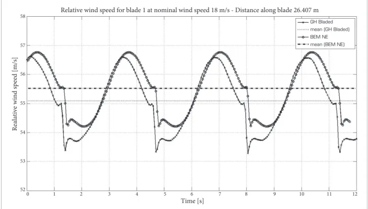
Results obtained until this point show a good correlation between the GH Bladed and the BEM NE for the wind speed 12 m/s. Now the same comparison of results for the wind speed 18 m/s is shown in the middle of the operation wind speed range. Figures 14 until 18 show these comparison. For wind speed 18 m/s the correspondent pitch angle is 14.9 degrees, as shown in Fig. 8.
Relative mean errors are compatible with the ones obtained for wind speed 12 m/s. he most important parameter, the shat power, has a relative error of -4.1%.
Figure 10. Angle of attack (wind speed 12 m/s).
Time [s]
Angle of attack [deg]
Angle of attack for blade 1 at wind speed 12 m/s - Distance along blade 26.407 m
0 1 2 3 4 5 6 7 8 9 10 11 12
7
6.5
6
5.5
5
4.5
4
3.5
GH Bladed mean (GH Bladed)
mean (BEM NE) BEM NE Figure 9. Inlow angle (wind speed 12 m/s).
Time [s]
Inlow angle [deg]
Inlow angle for blade 1 at wind speed 12 m/s - Distance along blade 26.407 m
0 1 2 3 4 5 6 7 8 9 10 11 12 11
10.5
10
9.5
9
8.5
8
7.5
GH Bladed mean (GH Bladed)
Figure 12. Lift coeficient (wind speed 12 m/s).
Time [s]
Angle of attack [deg]
Angle of attack for blade 1 at wind speed 12 m/s - Distance along blade 26.407 m
0 1 2 3 4 5 6 7 8 9 10 11 12
7
6.5
6
5.5
5
4.5
4
3.5
GH Bladed mean (GH Bladed)
mean (BEM NE) BEM NE Figure 11. Relative wind speed (12 m/s wind speed).
Time [s]
Relative wind speed [m/s]
Relative wind speed for blade 1 at wind speed 12 m/s - Distance along blade 26.407 m
0 1 2 3 4 5 6 7 8 9 10 11 12
55
54.5
54
53.5
53
52.5
52
GH Bladed mean (GH Bladed)
Figure 14. Inlow angle (wind speed 18 m/s).
Time [s]
Inlow angle [deg]
Inlow angle for blade 1 at wind speed 18 m/s - Distance along blade 26.407 m
0 1 2 3 4 5 6 7 8 9 10 11 12
22
21
20
19
18
17
16
15
GH Bladed mean (GH Bladed)
mean (BEM NE) BEM NE Figure 13. Measured shaft power (wind speed 12 m/s).
Time [s]
Angle of attack [deg]
Angle of attack for blade 1 at wind speed 12 m/s - Distance along blade 26.407 m
0 1 2 3 4 5 6 7 8 9 10 11 12
7
6.5
6
5.5
5
4.5
4
3.5
GH Bladed mean (GH Bladed)
Figure 16. Relative wind speed (wind speed 18 m/s).
Time [s]
Realative wind speed [m/s]
Relative wind speed for blade 1 at nominal wind speed 18 m/s - Distance along blade 26.407 m
0 1 2 3 4 5 6 7 8 9 10 11 12
58
57
56
55
54
53
52
GH Bladed mean (GH Bladed)
mean (BEM NE) BEM NE Time [s]
Angle of attack [deg]
Angle of attack for blade 1 at wind speed 18 m/s - Distance along blade 26.407 m
0 1 2 3 4 5 6 7 8 9 10 11 12
2
1
0
-1
-2
-3
-4
GH Bladed mean (GH Bladed)
mean (BEM NE) BEM NE
Figure 18. Measured shaft power (wind speed 18 m/s).
Time [s]
Measured shaft power [MW]
Measured shaft power at wind speed 18 m/s
0 1 2 3 4 5 6 7 8 9 10 11 12
2.2
2.15
2.1
2.05
2
1.95
1.9
1.85
GH Bladed mean (GH Bladed)
mean (BEM NE) BEM NE Time [s]
Lift coefficient
Lift coefficient for blade 1 at wind speed 18 m/s - Distance along blade 26.407 m
0 1 2 3 4 5 6 7 8 9 10 11 12
0.8
0.7
0.6
0.5
0.4
0.3
0.2
0.1
0
GH Bladed mean (GH Bladed)
mean (BEM NE) BEM NE
REFERENCES
Bisplinghoff, R. L., Ashley, H. and Halfman, R. L, 1955, “Aeroelasticity”, Addison-Wesley Publishing Co., Reading, MA.
Bramwell, A. R. S., Done, G. and Balmford, D., 1976, “Helicopter Dynamics”, Edward Arnold, Great Britain.
Burton,T., 2001, “Wind Energy Handbook”, Ed. John Wiley and Sons Ltd., Chichester, New York, 624 p.
Carpenter, P.J. and Fridovich, B., 1953, “Effect of A Rapid Blade-Pitch Increase on the Thrust and Induced-Velocity Response of a Full-Scale Helicopter Rotor”, NACA TN 3044.
Figure 19. Pitch angle for wind speed (a) 12 m/s and (b) 18 m/s from Bladed. Time [s]
Bladed Educational - Licensed to: Instituto
Tecnológico de Aeronáutica
0 2 4 6 8 10 12 0.80
0.78
0.76
0.74
0.72
0.70
0.68
0.66
0.64
Blade 1 pitch angle [deg]
Time [s]
Bladed Educational - Licensed to: Instituto
Tecnológico de Aeronáutica
0 2 4 6 8 10 12 15.02
15.00 14.98 14.96 14.94 14.92 14.90 14.88 14.86 14.84 14.82
Nominal pitch angle [deg]
(b) (a)
CONCLUSION
he work presented an alternative approach to predict the performance of upwind horizontal-axis wind turbine design using the unsteady BEM theory and an analytical model for the wake shed behind the rotor. his alternative approach is employed in order to verify the viability of using an analytical model for the returning wake efects, which does not have any empirical parameters or the need for experimental calibration. he numerical approach is very stable and fast, even being written in an interactive computation environment. he computational processing time necessary for any case is less than 10 seconds, and there were not numerical crashes. Based on the good approximation of results, when compared with others provided by commercial and established computational package, the mathematical model presented in this paper introduces an alternative tool for the wind turbine design, especially for upwind rotors.
he comparisons show that the model has good performance in terms of computational speed and the diferences between its results and those provided by the commercial sotware used as validation parameter are very small, being compatible with the optimization design method.
ACKNOWLEDGEMENTS
he authors acknowledge the inancial support from Coordenação de Aperfeiçoamento de Pessoal de Nível Superior (CAPES), by Programa Institucional de Qualiicação Docente para a Rede Federal de Educação Proissional e Tecnológica (PIQDTec), of Universidade Tecnológica Federal do Paraná (UTFPR).
Garrad Hassan & Partners, 2011, “Bladed Theory Manual Version 4.1 Multibody Dynamics”, St. Vincent’s Works, Silverthome Lane, Bristol BS2 0QD, England.
GL Garrad Hassan, 2012, http://www.gl-garradhassan.com.
Glauert, H., 1935, “Airplane Propellers”, Aerodynamic Theory (W.F. Durand, ed.), Div. L, Chapter XI. Berlin:Springer Verlag.
Glauert, H., 1929, “The Force and Moment on an Oscillating Airfoil”, Rep. Mem. Aeronaut., Res. Comm., Great Britain, No. 1561.
Hansen, M.O.L., 2007, “Aerodynamics of wind turbines”, Earthscan, Camden High Street London, NW1 0JH, UK, 2nd ed, pp 8-12.
Johnson,W., 1980, “Helicopter Theory”, Princeton University Press.
Jones, J.P., 1958, “The Inluence of the Wake on the Flutter and Vibration of Rotor Blades”, the Aeronaut. Quart., Vol. 9, No 3, pp 258-286.
Leishman, J.G., 2002, “Challenges in Modeling the Unsteady Aerodynamics of Wind Turbines”, 21st ASME Wind Energy Symposium and 40th AIAA Aerospace Sciences Meeting Reno, NV.
Leishman, J.G., 2000, “Principles of Helicopter Aerodynamics”, Cambridge University Press, The Edinburgh Building, Cambridge CB2 2RU, UK.
Loewy, R.G., 1957, “A Two-dimensional Approximation to the Unsteady Aerodynamics of Rotary Wings”, J. Aeronaut. Sci. Vol. 24, No 2, pp 81-92.
McGee, R.J. and Beasley, W.D., 1976, “The Aerodynamic Characteristics of An Initial Low-speed Family of Airfoils for General Aviation Applications”, NASA TM X-72843, NASA Langley Research Center, Hampton, VA, USA.