An impulsive framework for the control of hybrid systems
S´ergio Loureiro Fraga, Rui Gomes, Fernando Lobo Pereira
Abstract— An impulsive control formulation suitable for
analyzing hybrid systems is presented. Besides a continuous evolution, the trajectory of an impulsive control system may also exhibit jumps. The jump trajectory is well characterized in this impulsive framework. These jumps can be interpreted as the discrete evolution of an hybrid system. Several examples of hybrid systems modeled in the impulsive framework are given. An impulsive formulation of a formation control problem, regarded as an hybrid system is detailed. Finally, an overview of important classes of control results available for impulsive control systems, notably, stability and optimality, attest the importance of this paradigm for the control of hybrid systems. These results are essential to investigate the properties of model predictive control schemes for hybrid systems.
I. INTRODUCTION
Hybrid systems have been considered a convenient mod-eling framework to describe large classes of systems and extensively used in a wide range of applications, [1]. The trajectory of a hybrid system evolves as a result of the interaction between continuous and discrete dynamics. This interaction reflects the compositional properties underlying the hybrid system model.
On the other hand, an impulsive dynamic system can be regarded as a composition of multiple dynamic systems, and, hence, it is suited to model the behavior of some classes of hybrid systems. By exhibiting jumps in the trajectory, the impulsive control paradigm encompasses evolutions due to the interaction of continuous and discrete dynamics. A concept of trajectory that has been considered in [28], [25] provides a detailed description of a “path” joining the endpoints of any jump. This is required to ensure consistency of a solution to the measure driven dynamics.
The relationship between hybrid and impulsive systems enables the usage for hybrid control problems of a wealth of results available for impulsive systems [21], [22], [23], [27], [30], [29], [25], [4], [8], [18]. In [5], the relationship between differential impulsive inclusions and hybrid systems in the context of reachability and viability theory has been recognized. A distinguishing feature of this work and the one discussed here is precisely the way we describe the system behavior “during” the jump.
The article is organized in six sections. In section II, we introduce the impulsive control framework and discuss some key concepts and results. Then, in section III, we show how we can model hybrid systems as impulsive systems. We follow the taxonomy of [10] and we also use its examples
This work was supported by Fundac¸˜ao para a Ciˆencia e Tecnologia (FCT). The authors are with Instituto de Sistemas e Rob´otica - Porto, Faculdade de Engenharia, Universidade do Porto, Rua Dr. Roberto Frias s/n, 4200-465 Porto, Portugal{slfraga,rgomes,flp}@fe.up.pt
for illustrative purposes. In section IV, we give an on control of a formation, which may be seen as an hybrid system. It is formulated an optimal impulsive control problem in order to synthesize the formation controller. In section V, we discuss some of the main results on optimality as well as stability conditions for impulsive control systems. We close with some concluding remarks.
II. THE IMPULSIVE CONTROL FRAMEWORK
In our impulsive control framework we consider the fol-lowing class of measure driven dynamic control systems:
dx(t)∈f (t, x(t), u(t))dt+G(t, x(t))µ(dt), ∀t∈[0, 1] (1) with x(0) = x0, and where f : [0, 1]×Rn×Rm → Rn and
G : [0, 1]×Rn→ P(Rn×q) are given function and set-valued map, respectively. A control process for this system is a triple (x, u, µ) where the “conventional control” component u is a Borel measurable function satisfying u(t) ∈ Ut L-a.e. and
the impulsive control µ ∈ K is a nonnegative vector valued measure. K ⊂ C∗([0, 1]; K) is a convex cone of measures
with range in a pointed, convex cone K ⊂ Rq, i.e., µ(A) ∈
K for any Borel set A ⊂ [0, 1].
In what follows, we consider the canonical decomposition of the control measure
µ(dt) = wac(t)dt + wsc(t)|µsc|(dt) + µsa(dt), (2)
where wac(t)dt, µsc(dt), and µsa(dt), are, respectively,
the absolutely continuous, singular continuous and atomic components, |ν|(dt) denotes the total variation measure of the measure ν and wsc is the Radon-Nicodym derivative of
µsc w.r.t. its total variation measure.
The trajectory x ∈ BV+([0, 1]; Rn) is an Rn-valued
function on [0, 1], of bounded variation, which are continuous from the right on (0, 1], defined by x(0) = x0, and, ∀t > 0,
x(t) = xac(t) + xs(t) ∀t > 0 (3) where ˙xac(t) ∈ f (t, x(t), u(t))+G(t, x(t))wac(t), L − a.e. xs(t) = Z [0,t] G(t, x(t))wsc(t)|µsc|(dt)+ Z [0,t] ˜ g(t)|µsa|(dt).
Here, G is a µ-measurable selection of G and ˜g is defined by ˜ g(t) ∈ {|µsa|({t})−1[ξ(1) − ξ(0)] : ξ ∈ AC([0, 1]; Rn), ˙ξ(s) = G(t, ξ(s))v(s) a.e., ξ(0) = x(t−), (4) v(s) ∈ K, Z 1 0 v(s)ds = µsa({t})}.
This term clearly shows the final endpoint of a jump is a point in the state space that can be reached with the “singular dynamics” defined by G. This solves the apparent ill-posedness of the measure driven differential form (1) where, due to the discontinuity of x at time t, it is not clear a priori which value of x should be plugged in in the argument of G whenever the control measure µ has an atom.
Remark that the emergence of the “additional control” v is due to the non-uniqueness of the integral w.r.t. the measure µsa of the matrix-valued function G in the absence of the
commutativity property of the vector fields defined by its columns.
The driving control measure can be regarded as an ide-alization of a non-negative control that enters linearly into the dynamics and takes large values over small time subsets. The consistency of this concept requires the trajectory to be endowed with the property of robustness. By this, it is meant that solutions to dynamic system of equation (1) are “close” to solutions of a conventional differential equation in which µ is approximated by a conventional control m(t) associated with a measure via m(t)dt.
To be consistent with the interpretation of µ, we need to be sure that the state trajectory x corresponding to the idealized µ can be suitably approximated by a sequence of conventional trajectories corresponding to an approximating sequence of conventional controls, i.e.,
xi(t) → x(t), ∀t ∈ Cµ∪ {0, 1}, (5)
where Cµdenotes the points in [0, 1] which are not atoms of
µ, and {xi(t)} is a sequence of state trajectories, with initial
value x(0), corresponding to the sequence of conventional L-integrable controls {mi(t)}, with mi(t) ∈ K a.e. for each
i, and u(t) ∈ Ut, such that
mi(t)dt →∗µ(dt) weak∗. (6)
Here, weak∗ convergence means that
Z 1 0 h(t)mi(t)dt → Z [0,1] h(t)µ(dt), as i → ∞, (7) for every continuous function h on [0, 1].
This solution concept is a direct consequence of that defined in [24], [25] which extends the one developed in [28] that, in turn, follows the work in [16], [17] which use the reparameterization techniques in line with those in [27], [31].
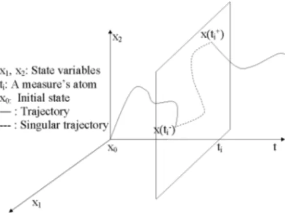
We also observe that this solution concept for the im-pulsive control system can be interpreted in terms of the composition of several dynamic systems which one driving the state variable subject to the “weight” dictated by the measure µ. In particular, when µ has an atom, the singular dynamics “explains” the path joining the trajectory jump endpoints. In figure 1, it is depicted an illustration of this solution concept.
Finally, we note that if the control measure µ is scalar-valued or the vector fields associated with the columns of the set valued map G are commutative (see [11]), then the definition of the jump becomes significantly simpler.
Fig. 1. Solution concept sketch for impulsive systems
III. HYBRID SYSTEMS MODELED AS IMPULSIVE CONTROL SYSTEMS
The impulsive solution concept described in the last sec-tion is not only amenable to a physical interpretasec-tion but also supports the analysis and control synthesis since is provided a characterization of the trajectory arc during the jump. Thus, instead of considering just a discrete transition in the state trajectory, in the impulsive formalism we also have the process that leads to that transition. Hence, if we model an hybrid system as an impulsive control system, then the results and methods associated with the later can be used to address hybrid systems.
We adopt the taxonomy for hybrid systems of [10] to show that impulsive systems formulation may model some classes of hybrid systems. We will give a formulation in terms of impulsive systems for the four classes of hybrid sys-tems of that taxonomy: autonomous switching, autonomous impulses, controlled switching and controlled impulses. For each of these classes, we will give the same example as in [10] using impulsive systems formulation for comparison purposes.
A. Autonomous switching
In this class of hybrid systems, the vector field may switch during the system operation. Thus, to model this situation we parameterize the vector field by a state variable q:
˙x(t) = f (t, x(t), u(t), q(t)), t ≥ 0. (8) We assume that vector field may also depend on time, state and control u. The parameter q is assumed to be a state variable that may change in discrete times
dq(t) = g(t, x(t))µ(dt). (9) The measure µ will be responsible for the switching and its support gives the instants where a transition in the vector field f happens :
supp µ = {t : φ(t, x(t)) = 0}. (10) Here, the function φ models the transition surface. There is a switching in the vector field whenever the state trajectory hits the surface defined by φ and this is the reason for the
designation autonomous switching. Obviously, there are an infinite number of possible locations q, which constitutes an advantage since more degrees of freedom are available to optimize any given objective function. However, we show in the next example that if finite number of locations is needed, it is possible to model that situation by defining trajectory constraints in the impulsive control problem.
Example 3.1: In this example we present a model of a dynamical system with hysteresis:
˙x = H(x) + u, (11)
where the state x and the control u are reals. The function H is an hysteresis having a threshold of ∆ and is depicted in figure 2 [10]. The impulsive control formulation is given by:
˙x = u + q, (12)
dq = −2σ(x)µ(dt), (13)
being σ a suitable Lipschitz continuous approximation to the signal function, q(0) ∈ {−1, 1} and the measure µ being characterized by
supp µ = {t : q(t)x(t) = ∆} (14) µ(dt) = δ(t − tµ), (15)
where tµ are the instants of measure’s support and δ is the
Dirac measure.
This impulsive model has the same behavior as the system of equation (11).
Fig. 2. Hysteresis function, [10]
B. Autonomous impulses
In this class of hybrid system, the state trajectory may exhibit a discontinuity when hitting prescribed regions of the state space. Once again, this situation may also be modeled as an impulsive system as follows:
dx ∈ f (t, x, u)dt + G(t, x)µ(dt) (16) being the measure supported on the set
supp µ = {t : θ(t, x(t)) = 0}. (17) where θ is a given function. The function f determines the system evolution in the continuous phase while set-valued map G defines the singular dynamics, which is responsible for determining the evolution of the state variable during the jump. The singular dynamics is the corresponding discrete evolution but with the added feature that, now, we have
infinitely many possible locations. In this formalism, the control of the jump is enabled by choosing appropriate selec-tions of G. The possible discrete locaselec-tions will correspond to points in the reachable set of the singular dynamics.
Example 3.2: In this example we consider a bouncing ball subject to gravity. When the ball hits floor, it changes abruptly its velocity due to the ground reaction force. Here, we consider the floor as a transition surface. Instead of only defining the final velocity after the impact we have, in the impulsive control formalism, a description of what happens during the jump. We model the impact by an under-damped linear spring. Thus, the impulsive model for this system is as follows:
dy = vdt + vµ(dt) (18)
dv = −gdt + (−ω2
ny − 2ωnζv)µ(dt) (19)
where ωn represents the natural frequency of the system
and ζ is called the damping coefficient and should be less than one. The damped natural frequency is given by ωd =
ωn
p
1 − ζ2. The measure is characterized by:
supp µ = {t : y(t) = 0} (20) µ(dt) = αδ(t − tµ). (21)
Note that, when the initial condition is such that y = 0 and v = 0, then the solution will be always ”evolving” due to the singular dynamics. Hence, the solution is well defined in the context of the robust solution concept introduced in section II. For this problem, the singular dynamics is simply a model of a linear spring with damping:
˙ys(s) = vs(s)α (22) ˙vs(s) = £ −ωn2ys(s) − 2ωnζvs(s) ¤ α, s ∈ [0, 1] (23) where α represents the total variation norm of the measure. In order to be consistent with the robust solution presented in section II and to avoid violate the trajectory constraint, the measure’s norm should be α = π
ωd (with this norm we will
have x = 0 for s = 1). Note that measure’s norm defines the time scaling of the singular dynamics. Due to this particular singular dynamics, the velocity at s = 1 will have its signal inverted in relation to the initial instant s = 0. Note that when no energy is lost during the impact, then damping coefficient is zero and the velocity after the impact just changes its signal without any attenuation.
In this example, we have seen that we may describe the system dynamics “during” the ideally instantaneous collision. This extra information may be beneficial in some circumstances. For example, imagine that we can control the surface orientation during the contact [7]. This orientation control leads to an extra control over the ball namely its orientation and angle of departure from the surface. If we had assumed no description of the arc jointing the jump points this control would not be possible.
C. Controlled Switching
Unlike in the autonomous switching case, in controlled switching hybrid systems the vector field of equation (8)
commutes not autonomously but in response to a control command. Thus, in the impulsive paradigm, instead of the measure be activated autonomously by predefining its support, it is defined by the controller. Once again, in the impulsive formalism the number of possible states q in equation (9) may be infinite. However, this formalism may also be applied in situations where it is required a finite number of vector fields. This is accomplished by introducing trajectory constraints as it is illustrated in the next examples. Example 3.3: Consider a simple satellite system where we can control the orientation by means of reaction jets:
˙ω(t) = τ v(t), t ≥ 0. (24) Here, ω is the angular speed, τ is the constant force applied by the jets and v ∈ {−1, 0, 1} is a variable that controls the direction of the jets (reverse, off and forward). This hybrid system can be formulated as an impulsive control system as follows: dω(t) = τ v(t)dt (25) dv(t) ∈ Aµ(dt) (26) subject to: −1 ≤ v(t) ≤ 1, v(0) ∈ {−1, 0, 1} (27) A ∈ {−2, −1, 1, 2}, µ(dt) = δ(t − tµ). (28)
We remark that tµ stands for the measure’s support instants.
As we can see from this example the measure’s support is not defined a priori and it is chosen by the controller. D. Controlled impulses
Hybrid systems of controlled impulses class are similar to the autonomous impulses except that now we do not have a pre-specification of the measure support. The state may jump whenever the controller activates the measure. We reinforce here that, by using the impulsive control formalism, we have a well defined description of the arc linking the point before and after the jump. This will enable us to develop results and methods for controller synthesis.
Example 3.4: We consider an inventory management model
dx(t) = −a(t)dt + µ(dt) (29) where x represents the stock level, the function a represents the stock consumption rate and the measure µ is the control variable that restores the stock level. By suitable choice of the measure support and norm we may control the level stock. An optimization problem could be defined to decide about the best strategy.
IV. CONTROL OF FORMATIONS
In the control of formations we have a network of vehicles that may interact between each other in order to define multiple configurations. Besides the continuous evolution of each element, these problems also include the control of the formation configuration. The change of configuration may be considered as a discrete transition. For this reason we may designate this type of control system as hybrid. Hence,
formations control is another class of problems for which we may use the impulsive formulation in order to derive an optimal controller. The formulation of this problem as an optimal impulsive control problem is part of our quest in establishing a bridge between hybrid and impulsive systems. The impulsive framework will enable the description of system’s trajectory during the reconfiguration period, which may be seen as an added feature in relation to conventional hybrid control formulation.
A. Network description
We wish to model a network where each node can position itself to make a formation with other nodes. There are dynamic constraints and optimizing costs that may cause the system to change the configuration. The problem concerns the computation of an optimal controller such that each component of the network must be as close as possible to a reference xr(t) while the network’s elements should
be as disperse as possible. These requirements models that the formation should follow a predefined trajectory while covering the biggest area possible (for inspection purposes for instance). The reconfiguration should be taken in a very short period. To simplify matters and focus on the impulsive benefits we will present an example where each node is modeled by one dimension dynamics.
B. Optimal impulsive control formulation
We show how we could model the previous problem as an optimal impulsive control problem. The dynamic model of each network component i is given by:
dxi(t) ∈ c(xi)dt + G(xi)µisa(dt), i = 1, .., N (30)
where the set-valued map G is given by:
G(x) := {g(x, u) : u ∈ [−1, 1]}. (31) The variable xi is the node’s position, the function c(x)
models deviations due to external modeled factors (wind, aquatic currents,...), the set-valued map models the node’s dynamics during the reconfiguration period while µi
samodels
the reconfiguration activation. For simplicity and without loss of generality, we assume similar dynamics for all network’s nodes. In this abstract model we assume the reconfiguration to be instantaneous which in practice means that each node has capacity for strong actuation during short periods of time (the µsa practical implementation). Due to the impulsive
solution concept we may say that the ’real’ trajectory is close to the ideal one in the sense described in section II.
The optimal impulsive control problem is formulated as follows: min µsa N X i=1 µZ 1 0 |xi(t) − xr(t)|2dt− − N X j=1,j6=i Z 1 0 |xi(t) − xj(t)|dt + Z [0,1] µi sa(dt) (32) subject to dynamic equation 30, with xi(0) = xi
0 for i =
The first component of the objective function models the tracking objective with reference trajectory xr, the second
component models the dispersion objective while the third component is an actuation cost. The square in the tracking objective is necessary to model the requirement of maxi-mizing communications between vehicles. Note that weights could be placed in the cost function to obtain different trade-offs.
We would like to emphasize that this impulsive framework is well suited for systems with discrete transitions but whose transition trajectory is also important to characterize. The previous example shows this issue since the network recon-figuration is viewed as a result of a ’strong’ actuation and consequently the transition’s trajectory is well characterized. Possibly, it would be possible to synthesize the controller for this formation with resource of the analytical results for impulsive systems, which are surveyed in the next section. However, this issue is out of scope of this paper. We expect to address this important issue in a future publication.
V. OVERVIEW OF SOME RESULTS
Previously, in section III, we presented the possibility of modeling hybrid systems by impulsive systems while in section IV we formulated an optimal impulsive control problem for an hybrid system. Now, we provide some insight on the relevance of this framework through an overview of some relevant results on impulsive systems. We will focus on conditions for optimality and for stability. These play a critical role on the design of optimality driven feedback control schemes such as model predictive control [6]. Al-though these schemes have been extremely successful for many conventional control problems, there is very little work for general nonlinear hybrid systems for which the proposed impulsive framework is particularly pertinent.
A. Optimality conditions
An impulsive optimal control problem may be formulated, in its more general form, as follows:
(P) min h(x(0), x(1))
subject to dynamics of equation (1) and to the constraints (x(0), x(1)) ∈ C, Φ(t, x(t)) ≤ 0, t ∈ [0, 1]. (33) Here, C is a closed subset of Rn×Rn and Φ : [0, 1]×Rn→
Rq and h : Rn× Rn → R are given functions.
Necessary and sufficient optimality conditions for variants of this problem already exist and may be useful to compute the optimal solution analytically. In one hand, necessary conditions have a local character and give clues about how to compute the measure’s support and the conventional control. On the other hand, sufficient conditions have a global character and involve the computation of the value function. Also, with optimality conditions at hand, it will be possible to explore numerical algorithms that approximates the analytical solution.
As a short overview, we mention that there are necessary conditions for problems without trajectory constraints where
set-valued map G does not depend on state x and the conventional control is assumed constant at measure’s atoms [27], [30]. When the set-valued map G is equal to a function g(t, x) and the measure is scalar we have the necessary conditions of [29]. In [25], [24] are given necessary con-ditions for measure driven differential inclusions. Necessary conditions considering trajectory constraints are addressed in [4], [3], [2]. In what concerns sufficient conditions of optimality, characterizations of the value function for variants of problem (P ) are given in [8], [14], [19], [20]. Also in [10], sufficient conditions of optimality were presented but the characterization of the singular dynamics was not considered. Necessary and sufficient conditions for optimal impulsive control problems of a different character have also been considered in [18].
B. Stability
Stability of hybrid systems has been subject of intensive research [13]. For switched systems, some authors have an-alyzed the possibility of using multiple Lyapunov functions for constructing a nontraditional Lyapunov function [9], [13]. In [9], for example, it is stated that if the derivative of the Lyapunov function of each vector field is nonincreasing and at the transition times the Lyapunov function is nonincreasing then we have stability. A less restrictive result is presented in [13] where it is allowed ”small” increases of the derivative of Lyapunov function in some vector fields provided other vector fields overcome this ”small” increase. At the transition instants it is only required that the value of the Lyapunov function of a vector field at the initial instant is lower than the last time that vector field was active (evaluated at the initial instant). Besides these results for switched systems, in [32] were also given stability results for systems having impulses. The more restrictive result states that the Lyapunov function derivative should be nonincreasing and in the discontinuities of the trajectory the value of the Lyapunov function is only allowed to decrease. In the more general result it is only required that during the jumps the Lyapunov function be nonincresing and in the continuous phase it is required that the Lyapunov function V be bounded by the combination of a prespecified bounded function and the right limit of V at the initial instant. We should mention that these results were developed without assuming any description of the singular dynamics.
For impulsive systems using the robust solution presented in section II there are two results concerning stability. In [21] and [22] are given sufficient conditions for asymptotically stability for impulsive control systems in terms of Lyapunov functions analogous to the one for conventional control systems (see for example [12]). The stability conditions were stated in [21] in terms of a control Lyapunov pair of functions satisfying the uniform decay condition. This is due to the fact that these conditions were found by applying ordinary stability theory to a standard problem obtained by a reparameterization of the original control system. The effect of these conditions in singular dynamics is that at measure’s atoms the Lyapunov function jumps downwards. However,
these conditions are useless in numerous cases since they are too restrictive. Therefore, in [22], this result is weakened and the notion of a controllable Lyapunov pair of functions is extended in such a way that V may increase at each jump. The price we pay for this approach is that we have to consider only control problems with a control measure such that either the total variation of its singular component is finite or its total variation on any finite interval tends to zero as its lower bound tends to infinity. This is a rather general scheme from the viewpoint of applications, although it might seem restrictive. This view is slightly different form the hybrid systems approaches since, here, we state that the continuous evolution of the system should compensate the eventual increase of the Lyapunov function value during the jumps.
When, for modeling reasons, it is necessary to model the singular dynamics, then the previous mentioned results on stability of impulsive systems are applicable. Besides this advantage, the solution concept presented in section II is robust in the sense that the set of solutions has closure properties with respect to the driving measure µ and the initial state [28]. These properties are crucial for deducing necessary optimality conditions and may also be useful for studying robust stability for hybrid systems. This robustness concept was introduced in [26] and the requirements for such solution were given in [15].
VI. CONCLUSION
A robust solution concept developed for impulsive con-trol systems was applied to model some classes of hybrid systems. Not only this solution concept may give additional modeling information due to the characterization of the tra-jectory during the jump but also it has robustness properties that allows the derivation of necessary optimality conditions in the form of a maximum principle.
There are still many open questions concerning issues related with the currently body of results discussed in this article which are required to design optimality based feedback control schemes such as model predictive control. Among these, it is of importance to establish results on the asymptotical optimization and on the stability of the synthesized controls. The robustness issue for the optimal controller is also an important issue that could be addressed using this impulsive framework.
REFERENCES
[1] Special issue on hybrid control systems, vol. 43, IEEE Transactions on Automatic Control, April 1998.
[2] A. Arutyunov, V. Dykhta, and F. Lobo Pereira, Necessary conditions
for impulsive nonlinear optimal control problems without a priori nor-mality asumptions, Journal of Optimization Theory and Applications
124 (2005), no. 1, 55–77.
[3] A. Arutyunov, V. Jacimovic, and F. Pereira, Second order necessary
conditions of optimality for impulsive control problems, International
Journal of Dynamic Control Systems 9 (2003), no. 1, 131–153. [4] A. Arutyunov, D. Karamzin, and F. Pereira, A nondegenerate maximum
principle for impulse control problem with state constraints, SIAM
Journal of Control and Optimization 43 (2005), no. 5, 1812–1843. [5] J.P. Aubin, J. Lygeros, M. Quincampoix, S. Sastry, and N. Seube,
Impulse differential inclusions: a viability approach to hybrid systems,
IEEE Transactions on Automatic Control 47 (2002), no. 1, 2–20.
[6] A. Bemporad and M. Morari, Control of systems integrating logic,
dynamics, and constraints, Automatica 35 (1999), no. 3, 407–427.
[7] J. Bentsman and B.M. Miller, Dynamical systems with controlled
singularities: physically based representation and control-oriented modeling, 42nd IEEE Conference on Decision and Control, vol. 6,
2003, pp. 6351– 6356.
[8] Daniel P. Berovic and Richard B. Vinter, The application of dynamic
programming to optimal inventory control, IEEE Transactions on
Automatic Control 49 (2004), 676–685.
[9] Michael S. Branicky, Multiple lyapunov functions and other analysis
tools for switched and hybrid systems, IEEE Transactions on
Auto-matic Control 43 (1998), no. 4, 475–482.
[10] M.S. Branicky, V.S. Borkar, and S.K. Mitter, A unified framework for
hybrid control: model and optimal control theory, IEEE Transactions
on Automatic Control 43 (1998), 31–45.
[11] Alberto Bressan, Impulsive control of lagrangian systems and
loco-motion in fluids, http://www.math.psu.edu/bressan/, 2006.
[12] F. H. Clarke, Yu. S. Ledyaev, R. J. Stern, and P. R. Wolenski,
Nonsmooth analysis and control theory, Springer, 1998.
[13] Raymond A. Decarlo, Michael S. Branicky, Stefan Pettersson, and Bengt Lennartson, Perspectives and results on the stability and
stabi-lizability of hybrid systems, Proceedings of the IEEE 88 (2000), no. 7,
1069–1082.
[14] Grant N. Galbraith1 and Richard B. Vinter, Optimal control of hybrid
systems with an infinite set of discrete states, Journal of Dynamical
and Control Systems 9 (2003), no. 4, 563–584.
[15] R. Goebel, J. Hespanha, A.R. Teel, C. Cai, and R. Sanfelice, Hybrid
systems: generalized solutions and robust stability, In IFAC
Sympo-sium Nonlinear Control Systems (2004).
[16] G. Dal Maso and F. Rampazzo, On systems of ordinary differential
equations with measures as controls, Differential and Integral
Equa-tions 4 (1991), 739–765.
[17] Boris M. Miller, The generalized solutions of nonlinear optimization
problems with impulse control, SIAM Journal of Control and
Opti-mization 34 (1996), no. 4, 1420–1440.
[18] Boris M. Miller and Evgeny Y. Rubinovich, Impulsive control in
continuous and discrete-continuous systems, Kluwer Academic
Pub-lishers, Amsterdam, Holland, 2003.
[19] Monica Motta and Franco Rampazzo, Dynamic programming for
nonlinear systems driven by ordinary and impulsive controls, SIAM
Journal on Control and Optimization 34 (1996), no. 1, 199–225. [20] , The value function of a slow growth control problem with
state constraints, Journal of Mathematical Systems, Estimation and
Control 7 (1997), no. 3, 1–20.
[21] F. Lobo Pereira and Geraldo N. Silva, Stability for impulsive control
systems, Dynamical Systems 17 (2002), no. 4, 421–434.
[22] , Lyapounov stability of measure driven differential inclusions, Journal of Differential Equations 40 (2004), no. 8, 11221130. [23] F. Lobo Pereira, Geraldo N. Silva, and Valeriano Oliveira, Invariance
for impulsive control systems, Automation and Remote Control (2007).
[24] Fernando Lobo Pereira and Jorge Morais Leite, Necessary conditions
of optimality for impulsive control problems with state constraints,
European Control Conference, 2007.
[25] Fernando Lobo Pereira and Geraldo Nunes Silva, Necessary conditions
of optimality for vector-valued impulsive control problems, Systems
and Control Letters, Elsevier 40 (2000), 205–215.
[26] Christophe Prieur, Perturbed hybrid systems, applications in control
theory, Nonlinear and Adaptive Control 281 (2003), 285–294.
[27] Raymond W. Rishel, An extended pontryagin principle for control
systems whose control laws contain measures, SIAM Journal of
Control 3 (1965), no. 2, 191–205.
[28] G. N. Silva and R. B. Vinter, Measure differential inclusions, Journal of Mathematical Analysis and Applications (1996), no. 202, 727–746. [29] , Necessary conditions for optimal impulsive control problems, SIAM Journal of Control and Optimization 35 (1997), no. 6, 1829– 1846.
[30] R. B. Vinter and F. M. F. L. Pereira, A maximum principle for optimal
control processes with discontinuous trajectories, SIAM Journal of
Control and Optimization 26 (1988), no. 1, 205–229.
[31] J. Warga, Optimal control of differential and functional equations, Academic Press, NewYork, 1972.
[32] Hui Ye, Anthony N. Michel, and Ling Hou, Stability analysis of
systems with impulse effects, IEEE Transactions on Automatic Control
![Fig. 2. Hysteresis function, [10]](https://thumb-eu.123doks.com/thumbv2/123dok_br/19175755.943105/3.918.134.400.620.745/fig-hysteresis-function.webp)
