Vol. 34, No. 04, pp. 1149 – 1159, October – December, 2017 dx.doi.org/10.1590/0104-6632.20170344s20160158
1 A preliminary version of this work was presented at the Terceras Jornadas Argentinas de Seguridad de Procesos, Buenos Aires, 2015.
DISCHARGE OF NON-REACTIVE
FLUIDS FROM VESSELS
1
M. Castier
1
,*, A. Basha, R. Kanes
1
and L.N. Véchot
1
1Mary Kay O’Connor Process Safety Center. Chemical Engineering Program, Texas A&M University at Qatar P.O. Box 23874, Doha - Qatar
*Corresponding author: E-mail [email protected]; Phone: +974-44230534; Fax: +974-44230065
(Submitted: March 7, 2016; Revised: June 29, 2016; Accepted: August 7, 2016)
Abstract – This paper presents simulations of discharges from pressure vessels that consistently account for non-ideal
fluid behavior in all the required thermodynamic properties and individually considers all the chemical components
present. The underlying assumption is that phase equilibrium occurs instantaneously inside the vessel and, thus, the
dynamics of the fluid in the vessel comprises a sequence of equilibrium states. The formulation leads to a system of differential-algebraic equations in which the component mass balances and the energy balance are ordinary differential
equations. The algebraic equations account for the phase equilibrium conditions inside the vessel and at the discharge point, and for sound speed calculations. The simulator allows detailed predictions of the condition inside the vessel and
at the discharge point as a function of time, including the flow rate and composition of the discharge. The paper presents conceptual applications of the simulator to predict the effect of leaks from vessels containing mixtures of light gases
and/or hydrocarbons and comparisons to experimental data.
Keywords: Relief, venting, tank, valve, equation of state.
INTRODUCTION
Discharges of hazardous chemicals can bring about serious consequences to populations living close to industrial units, in addition to financial losses. In some cases, the discharges are accidental, as in the case of leaks. In others, as in operations for pressure relief, they are intentional and aim to prevent further damage, such as the explosion of pressure vessels. In both cases, it is important to predict the flow and composition of the material discharged to the environment in order to plan measures of containment and remediation.
Due to the growing importance of this practical problem, several programs for the simulation of leaks and venting from pressure vessels exist (Woodward and Mudan, 1990; Bendiksen et al., 1991; Haque et al., 1992a, 1992b; Richardson and Saville, 1996; Mahgerefteh and
Wong, 1999; Cumber, 2001; Witlox and Bowen, 2002; Renfro et al., 2014; D’Alessandro et al., 2015). In order to simplify the formulation and shorten their execution time, some of them use approximations, such as that of ideal gas behavior, that increase the uncertainty of their predictions. Other papers account for deviations from ideal gas behavior as, for example, those of Haque et al. (1992a, 1992b) and Richardson and Saville (1996), who used a proprietary computer package for physical properties called PREPROP, and of Mahgerefteh and Wong (1999), who used cubic equations of state. Another approximation occasionally used is that the chemical components can be lumped into a single pseudo-component; however, the composition of the vented fluid and of the fluid inside the vessel can vary significantly during a simulated period. These references focus on the so-called source term, which refers to the behavior of the fluid up to the point
of Chemical
of its release from the vessel. The behavior of the fluid beyond the release point can also be rather complex, as exemplified by the work of Birch et al. (1987), who present correlations to predict how the velocity of the fluid decays as it flows into the atmosphere. Other examples are the work of Winters (2009) and Houf and Winters (2013), who model the flow of hydrogen into ambient air right after leaks from tanks that store liquid hydrogen at very low temperatures. An interesting aspect of these publications is the rigorous modeling of physical properties using the REFPROP (Lemmon et al., 2007) thermodynamics suite of flash algorithms.
Renfro et al. (2014) describe the features of the “Blowdown Utility” program for the simulation of discharges from horizontal or vertical vessels of several geometries. A non-equilibrium vessel model is adopted and the simulator allows the choice of several models for the evaluation of the physical properties of the fluid. Their approach allows the simulation of vessels that contain three fluid phases. However, the article provides no details about the mathematical formulation and an undisclosed expression is used to calculate the flow rate of the leaking fluid.
D’Alessandro et al. (2015) describe a simulator called VBsim (Vessel Blowdown Simulator) that uses global phase stability analysis and minimization of the Gibbs energy to find the conditions inside the vessel. VBsim uses the concept of partial phase equilibrium (Speranza and Terenzi, 2005), according to which the liquid and vapor phases have the same pressure, but not the same temperature, because of their different heat transfer coefficients, which are calculated by the program. In this approach, the liquid phase is in equilibrium with a “bubble” phase while the vapor phase is in equilibrium with a “droplet” phase. Different expressions are adopted for the flow through the vessel’s orifice, depending on whether the discharge is of a liquid or vapor phase. However, their approach seemingly disregards the possibility of phase change at the discharge point.
This paper introduces a simulator for discharges from pressure vessels that accounts for deviations from ideal gas behavior in all the required thermodynamic properties and individually considers all the chemical components present. The formulation follows the so-called homogenous equilibrium assumption, according to which equilibrium is achieved instantaneously and, thus, the dynamics of the fluid in the vessel comprises a sequence of equilibrium states. The underlying mathematical problem is a system of differential-algebraic equations (DAE) in which the component mass balances and the energy balance are ordinary differential equations. The differential energy balance includes the internal energy of the fluid and of the vessel walls. The algebraic equations account for the phase equilibrium conditions inside the vessel and at the discharge point. Due to the size and complexity of the model, numerical solution is necessary.
At each time step during the integration of the ordinary differential equations of the model, the values of the internal energy and component amounts inside the vessel become known. Since the vessel’s volume is known and fixed, the state of the system can be found by maximizing the fluid’s entropy (Callen, 1985). To compute the discharge conditions, the assumption is that the region inside the vessel close to the discharge point acts as an adiabatic converging nozzle whose operation is isentropic. This leads to an unusual equilibrium problem with specification of fluid entropy and stagnation enthalpy (enthalpy plus kinetic energy). The model accounts for the possibility of non-choked and choked flow at the discharge point. In the latter, the fluid speed is equal to the local thermodynamic sound speed. Therefore, a procedure to compute the thermodynamic sound speed in systems with multiple phases is also part of the formulation.
The simulator allows predictions of the conditions inside the vessel and at the discharge point as a function of time, including the flow rate and composition of the discharge, which are crucial pieces of information when planning for emergencies and studying containment alternatives. The paper shows applications of the simulator to predict the effect of leaks from vessels containing light gases and hydrocarbon mixtures.
ASSUMPTIONS
A set of assumptions underlies the development of the mathematical model of leak and vent operations from pressure vessels. A central one is that the fluid inside the vessel is in thermodynamic equilibrium at all times, and that properties such as temperature, pressure, and chemical potential of each component are the same everywhere within the vessel. When the mass and the specific heat capacity of the vessel wall are considered in the simulation, it is assumed that the wall and fluid temperatures are equal at any time. It is also assumed that the volume of the vessel’s wall remains constant, that is, wall expansions or contractions because of temperature changes are neglected. In the absence of chemical reactions, as is the case considered here, this means that determining the state of the fluid within the vessel requires a phase equilibrium computation.
With these assumptions, the mathematical model consists of a set of differential-algebraic equations (DAE). The mass and energy balances are ordinary differential equations (ODE). The algebraic equations allow the determination of the state of the fluid inside the vessel and at the exit point at each time step of the numerical ODE integration.
Furthermore, to determine the leak or vent flow rate, it is necessary to find several fluid properties at the fluid’s exit point from the vessel, namely, its temperature, pressure, number of phases with their amounts and compositions, and thermodynamic sound speed. The sound speed is relevant because it is the maximum achievable fluid speed at the exit of a converging nozzle. Flows at sonic speed are referred to as choked and the pressure at the exit point is larger than the backpressure, which is the environmental pressure away from the vessel. Flows below sonic speed are referred to as non-choked and the exit pressure is equal to the backpressure.
FORMULATION
The formulation follows the recent work of Kanes et al. (2016). We consider storage vessels with no material input during the simulated time. The number of output streams is arbitrary and user-defined. The possibility of simulating the simultaneous discharge through more than one output stream is useful in situations such as the aperture of a relief valve followed by the opening of a bursting disk. We consider vertical cylindrical vessels; if the phase volumes are known, it is simple to compute the level of the interfaces. By knowing these levels and the shape and position of the orifices, it is possible to determine the leaking phase at any given moment. This may change during the simulation. For example, at the beginning of a simulation, the liquid phase may leak but, as its level decreases, vapor may leave the vessel through the same orifice in later stages of the process. In this paper, we assume that the orifice sizes remain constant during the simulated time.
The first step of the solution procedure is to determine the initial condition of the fluid in the vessel. This is accomplished by solving a flash calculation whose specifications are the fluid temperature, internal volume of the vessel, and amount of each component (Espósito et al., 2000). By minimizing the system’s Helmholtz energy and using global phase stability analysis (Michelsen, 1982), this calculation determines the number of phases present, their volumes, amounts, compositions, and internal energies at the beginning of the simulated process. When the effect of the vessel wall is included in the simulation, determining the initial condition includes the evaluation of the wall’s internal energy, given its mass and specific heat capacity at constant volume.
With the initial state determined, it is possible to start the dynamic simulation of the fluid in the vessel, which
requires the solution of a set of differential equations. The differential mass balance of each component
i
, written on a molar basis, is:1
out
ns out i
im m
dn
n
dt
== −
∑
In Eq. (1),
t
represents time,n
i is the number of molesof component i in the vessel, and
n
imout is the molar flowrate of component i in stream m, which is one of the
ns
outstreams that exit the vessel. The energy balance takes the form:
( )
21
2
out out
ns
m out out out m m m m
u
dU
n
h
M
Q
dt
=
= −
+
+
∑
In Eq. (2),
U
is the internal energy of the vessel wall(when it is considered) and of the fluid in the vessel,
Q
is the heat transfer to the fluid in the vessel, and outm
h
,out m
M
, andu
moutare the molar enthalpy, molar mass,and average fluid speed at exit point m, respectively. It is necessary to apply a numerical method to integrate the ODE set comprised by Eqs. (1) and (2). In this work, the Bulirsch-Stoer method is used, as implemented by Press et al. (1992). This is a conventional ODE integrator, not an integrator for differential algebraic equations (DAE). There has been no attempt to use a DAE integrator because reliable numerical convergence of phase equilibrium equations (algebraic) often requires highly specialized algorithms. The adopted strategy has been to solve the algebraic equations every time the ODE integrator needs to evaluate the right hand side of the differential mass and energy balances, which are represented by Eqs. (1) and (2), respectively. To compute them, it is necessary to determine the flow rate, composition, average fluid speed, and
enthalpy of each stream m that exits the vessel. All these
algebraic calculations consider the possibility of single or multiple phases in the vessel and at the exit point.
The first step to accomplish that is to determine the state of fluid in the vessel. This requires solving a flash problem whose specifications are the current values of internal energy and component amounts, as provided by the ODE integrator, and the vessel’s internal volume, which is constant. Determining the equilibrium condition for this set of specifications requires maximizing the system’s entropy (Callen, 1985). A flash algorithm developed specifically for this situation (Castier, 2009) is used. This (1)
algorithm is extended in this work to account for cases that include the mass and heat capacity of the vessel wall, which is considered as a solid phase that exchanges heat, but neither mass nor volume, with the fluid phases present. The outcomes of this calculation are the fluid and wall temperature and fluid pressure, number of phases present, their densities and volumes, amount of each component in each phase, and the molar enthalpy and entropy of each phase, among other thermodynamic properties. With the calculated phase volumes (and mass densities, to establish their relative positions), it is possible to find the location of the interfaces for a given vessel geometry (vertical cylinder,
in this work). The position of each exit point m is then
checked against the interface locations to decide whether each discharge is from a liquid or vapor phase, or both when an orifice is exposed to both phases simultaneously, as discussed by Kanes et al. (2016).
The next step is to model what happens inside the vessel
next to each exit point m. The assumptions are that each of
these regions behaves as a converging nozzle that operates adiabatically and isentropically and that changes to the nozzle’s input conditions have instantaneous effect on the exit conditions, i.e., mass and energy accumulations in the nozzle are neglected. An additional assumption is that the average fluid speed at the nozzle’s entrance is negligible compared to its value at the exit point. These assumptions lead to the following two algebraic equations, written on a molar basis:
( )
22
out m dch out out
m m
u
h
=
h
+
M
dch out m
s
=
s
where the superscript dch denotes properties of the
discharged material inside the vessel, at the entrance of the hypothetical nozzle. It should be noted that the fluid may have one or more phases at an exit point, but this is not known beforehand. In fact, determining the state of a fluid with specifications of fluid composition, entropy, and stagnation enthalpy constitutes an unusual phase equilibrium problem. A new algorithm for this situation has been the focus of recent work (Castier et al., 2016). An important feature of this algorithm is that it begins with the assumption that the pressure at the exit point is equal to the specified value of the backpressure. If it turns out that the flow is supersonic under these considerations, the solution is invalid because the sound speed is the upper limit for flow speed at the exit of an adiabatic converging nozzle. When this happens, the problem is solved again relaxing the pressure specification and considering that the flow is sonic. Thus, the sound speed calculations play an important
role on the overall computation path. Very importantly, they are occasionally necessary for systems with more than one phase, if flashing conditions occur at the exit point. Few algorithms exist to this end. A recent procedure for the calculation of thermodynamic sound speed in systems with any number of fluid phases (Castier, 2011) is used in this work. For multiphase systems, this procedure involves the solution of a system of linear equations formulated with the use of derivatives of several thermodynamic properties, phase equilibrium conditions, and conservation equations for volume, entropy, and mole number of each component. Regardless of being sonic or subsonic, the flow rate at the exit point is obtained using:
out out out m m m out
m
A u
v
n
=
where
A
mout andv
mout are the exit area and molar volumeat point m, respectively.
In summary, three flash algorithms are necessary as part of these simulations:
• A TVN flash establishes the initial state of the fluid in
the vessel for given volume, initial temperature, and initial amounts of each component.
• A UVN flash determines the state of the fluid in the
vessel during the dynamic simulation. Its specifications are the current values of U and N obtained from the numerical integration of the differential equations and the internal vessel volume, which is constant throughout the simulated period.
• A HSN flash determines the state of the fluid at the leak
point, which is assumed to be the exit of a hypothetical converging nozzle. Its specifications are the stagnation enthalpy of the fluid that enters the nozzle, its entropy, and component amounts.
In this work, the Peng-Robinson equation of state (Peng and Robinson, 1976) is used to compute the thermodynamic properties, including the fugacity coefficients, residual internal energy, residual enthalpy, residual entropy, and thermodynamic sound speed, as well as their derivatives, as required by the phase equilibrium calculations. In this sense, the same thermodynamic model is used to evaluate all the thermodynamic properties of the fluid. The critical properties, acentric factor, and coefficients of a 3rd degree
polynomial correlation in temperature for the molar ideal gas heat capacities are taken from Reid et al. (1987). Despite the specific modeling choices, it should be noted that the formulation is general and not limited to using the Peng-Robinson equation of state, whose recommended application is for calculations involving hydrocarbon mixtures.
(3)
(4)
RESULTS
This section shows simulation results of cases in which light gases or hydrocarbons are vented from vertical cylindrical vessels. The possible occurrence of chemical reactions is neglected in all cases.
Discharge of nitrogen or methane
This conceptual case compares the discharge of pure nitrogen or pure methane. The vessel is adiabatic and has
a volume of 1.00 m3, with height of 2.00 m and diameter
of 0.798 m. A 25.0x10⁻⁶ m2 orifice located 1.00 m above
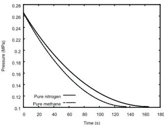
the bottom of the vessel is used (with unity coefficient of discharge). The initial temperature of the fluid in the vessel’s interior is 400 K. The vessel load consists of 80.0 moles of nitrogen or methane and the thermal inertia of the vessel walls is neglected. Figure 1 shows how the pressure inside the vessel drops as function of time until it becomes equal to the backpressure, which is specified to be equal to 0.10132 MPa. It is noticeable that the discharge of nitrogen takes longer, which is an outcome associated to the fluid speed at the exit point.
Figure 2 displays the corresponding temperature profile during the simulated period. Methane has larger molar heat capacity than nitrogen and its temperature drop is accordingly smaller.
Figure 3 shows the fluid and sound speeds at the point of discharge. For each compound, these speeds overlap in the beginning of the simulated time, until 38.7 s for methane and 40.5 s for nitrogen, meaning that the exit flow is sonic, i.e., choked. The plot also shows that the discharge speed of pure methane is faster than that of pure nitrogen, justifying the fact that the pressure in the methane vessel becomes equal to the backpressure before this happens in the nitrogen vessel (Fig. 1).
Therefore, these results illustrate how two pure light compounds behave differently during a leak, even though there is only one phase inside the vessel and at the exit point for both of them throughout the simulated period.
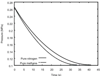
Figure 4 shows the effect of increasing the orifice area
to 100.0x10⁻⁶m2, i.e., quadrupling its area compared to
the previous situations. As expected, the times needed to equalize the vessel pressure and the backpressure are one-fourth of the times reported in Fig. 1.
Discharge of nitrogen: comparison with Véchot’s (2006) data
Véchot (2006) measured temperature and pressure
during the discharge of nitrogen from a 0.0107 m3
vessel initially at 0.3612 MPa and 293.67 K through an orifice whose area is equal to 1.131x10⁻⁶ m2. To match
these specifications, the initial amount of nitrogen in the simulation is equal to 1.586 moles of nitrogen.
For an adiabatic vessel of negligible heat capacity compared to the heat capacity of the fluid it contains, the
0.1 0.12 0.14 0.16 0.18 0.2 0.22 0.24 0.26 0.28
0 20 40 60 80 100 120 140 160 180
Pressure (MPa)
Time (s) Pure nitrogen
Pure methane
Figure 1. Pressure in vessels loaded with either pure nitrogen or pure methane.
300 310 320 330 340 350 360 370 380 390 400
0 20 40 60 80 100 120 140 160 180
Temperature (K)
Time (s) Pure nitrogen
Pure methane
Figure 2. Temperature in vessels loaded with either pure nitrogen or pure methane.
0 50 100 150 200 250 300 350 400 450 500
0 20 40 60 80 100 120 140 160 180
Speed (m/s)
Pure nitrogen
Sound speed in nitrogen
Pure methane
Sound speed in methane
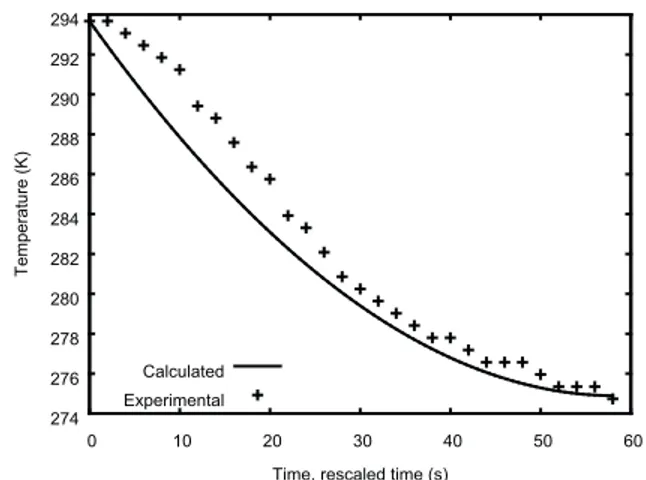
fluid temperature would decrease from the beginning until the end of the experiment. The experimental data show that there is a minimum in temperature equal to 274.73 K at 58 s. The nitrogen temperature increases after that, indicating that there is heat transfer to the fluid in the vessel, either from outside the system or from the vessel’s construction material. As Véchot (2006) did not report the mass and material of construction of the vessel, this effect was simulated by imposing a constant heat transfer rate to the fluid (equal to 41 J/s) so that the simulated temperature exhibits the same minimum value, which occurs at 28.9 s of simulated time. The ratio of the simulated and experimental times for the minimum in temperature, equal to 0.50, was interpreted as a practical coefficient of discharge for this venting process, which is lower than the typical value of 0.61 for discharges through orifices.
Figures 5 and 6 display the pressure and temperature profiles. There is only one phase within the vessel during the simulated period. The experimental data are plotted against the measured time. The calculated data are plotted against a rescaled time equal to the simulated time divided by the coefficient of discharge of 0.50. The plots end at 58 s, when the minimum in temperature occurs. The experimental and calculated results are in acceptable agreement during this period. Beyond it, the disagreement between the two results increases, especially for temperature, because of the adopted approximation of constant heat transfer rate.
Discharge of nitrogen: comparison with Haque et al.’s (1992b) data
Haque et al. (1992b) measured the gas temperature, wall temperature, and pressure during the discharge of nitrogen, initially at 15.0 MPa and 290 K, from a vessel of undisclosed construction and insulating (if any) materials. Haque et al. (1992b) report the following vessel dimensions: height of 1.524 m, internal diameter of 0.273 m, wall thickness of 0.025 m, with a circular orifice whose diameter is 0.00635 m, positioned at the top of the vessel. Using these dimensions and assuming that the vessel is of stainless steel 316, whose density was taken as equal
to 7950 kg/m3 (British Stainless Steel Association, 2016),
the vessel’s mass was estimated to be equal to 316.1 kg. To match the problem specifications, the initial amount of nitrogen in the simulation is equal to 557.3 moles, which
corresponds to 15.60 kg. Thus, under these assumptions, the initial mass of nitrogen is just 4.7% of the total mass of the system. The vessel is considered as adiabatic and the internal energy of the solid is considered in the simulation, with the specific heat capacity of steel at constant volume calculated using the following third degree polynomial in temperature (in Kelvin):
0.18 0.2 0.22 0.24 0.26 0.28 0.3 0.32 0.34 0.36 0.38
0 10 20 30 40 50 60
Pressure (MPa)
Time, rescaled time (s) Calculated
Experimental
Figure 5. Pressure in a vessel loaded with nitrogen: comparison of experimental (Véchot, 2006) and calculated values.
0.1 0.12 0.14 0.16 0.18 0.2 0.22 0.24 0.26 0.28
0 5 10 15 20 25 30 35 40 45
Pressure (MPa)
Time (s) Pure nitrogen
Pure methane
Figure 4. Pressure in vessels loaded with either pure nitrogen or pure methane: effect of larger orifice.
(6)
3 2 7 3
174.59 1.3837
1.7172 10
7.6188 10
.
v
J
c
T
T
K
T
kg
− −
+
−
=
×
+
×
This expression fits experimental data (British Stainless Steel Association, 2016) between 293.15 K to 1143.15 K with an absolute average relative deviation of 0.30%.
Figures 7 displays the experimental pressure data as
274 276 278 280 282 284 286 288 290 292 294
0 10 20 30 40 50 60
Temperature (K)
Time, rescaled time (s) Calculated
Experimental
Figure 6. Temperature in a vessel loaded with nitrogen: comparison of experimental (Véchot, 2006) and calculated values.
0 2 4 6 8 10 12 14 16
0 20 40 60 80 100
Pressure (MPa)
Time, rescaled time (s)
Calculated
Experimental
Figure 7. Pressure in a vessel loaded with nitrogen: comparison of experimental (Haque et al., 1992b) and calculated values.
0.1 0.15 0.2 0.25 0.3 0.35 0.4
0 100 200 300 400 500 600 700 800 900
Pressure (MPa)
Time (s)
Figure 8. Pressure in a vessel loaded with equimolar nitrogen+methane mixture: effect of opening a relief valve and a bursting disk.
a coefficient of discharge of 0.70, in such a way that the final rescaled time at the end of the run is also equal to 100 seconds. At this condition, the simulated pressure inside the vessel becomes equal to the atmospheric pressure. The model overestimates the pressure at 10 s and 20 s, but there is good agreement between the experimental and calculated pressures at later times.
Concerning temperature, the experimental data of Haque et al. (1992b) show that the fluid temperature passes through a minimum, of about 190 K, and then increases, reaching a temperature of about 220 K at the end of the experiment. A possible explanation for this behavior is heat transfer from the vessel walls to the fluid, counteracting the temperature drop caused by depressurization. The experimental value of the wall temperature drops throughout the experiment, reaching a final value of about 285 K. As the model assumes a single temperature for the whole system, it cannot predict different temperatures for the fluid and for the wall. The simulated temperature results show a steady decrease in temperature from the initial temperature of 290 K to a final temperature of 279.6 K. This shows that the thermal inertia of the vessel wall, whose mass is about 20 times the mass of nitrogen, dominates the model’s temperature prediction. Thus, the temperature from the simulation is between the experimental fluid and wall temperatures, but closer to the latter because of the large heat capacity of the vessel wall.
Discharge of nitrogen+methane mixture from heated vessel
This conceptual case considers the discharge of an equimolar mixture of nitrogen and methane from a vessel of the same size and shape as that of case 4.1, with the binary interaction parameter of the Peng-Robinson EOS set to 0.1 (Firoozabadi, 1999). The vessel initially contains 40 moles of each compound at the temperature of 400 K. There is heat transfer to the fluid in the vessel at a rate of 1000 J/s. The vessel is initially closed and a relief valve
(25.0x10⁻⁶ m2, located 1.0 m above the bottom) opens when
the pressure reaches 0.35 MPa. A bursting disk (100.0x10
-6m2, located 1.5 m above the bottom) opens when the
pressure reaches 0.40 MPa. Unity coefficient of discharges were used for the relief valve and busting disk.
Figure 9 shows the fluid temperature during the simulated period. The opening of the relief valve has little effect on the temperature but, when the bursting disk opens, it drops sharply.
Figure 10 is a plot of the total molar amount within the vessel as a function of time. The amount is initially constant and equal to 80 moles because the vessel is closed; it then undergoes a small decrease while the valve relief is open but the bursting disk is closed, and finally decreases rapidly when both are open.
Figure 11 shows the fluid and sound speeds. The relief valve opens at about 293 s of simulated time. Between this time and the time the bursting disk opens, at about 795 s, the flow is sonic and of increasing velocity. Shortly after the opening of the bursting disk, at about 815 s, the flow becomes subsonic. It should be noted that the flow and sound speeds in the relief valve and in the bursting disk, when both are open, are identical. This happens because there is only one phase within the vessel at all times and, therefore, the properties of the fluid vented through both devices are equal.
Discharge of a two-phase n-hexane+n-octane mixture
This conceptual case simulates the discharge of an equimolar mixture of n-hexane+n-octane from an adiabatic
vessel whose volume is 0.7894 m3, with height of 1.00 m
and diameter of 1.00 m. The binary interaction parameter of the Peng-Robinson EOS was set to zero, as usual for hydrocarbon mixtures (Reid et al, 1987). The orifice has an
area of 12.57x10⁻⁶m2, centered 0.50 m above the vessel’s
bottom. The initial temperature of the fluid in its interior is 400 K. The load consists of 100 moles of each component and the coefficient of discharge is equal to 1. This section presents results of two cases with different initial fluid temperatures, equal to 450 K and 460 K. In both of them, the fluid has two phases inside the vessel at the beginning of the simulated period. However, the liquid level is low and the leak is from the vapor phase at all times.
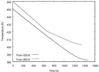
Figures 12 and 13 show the evolution of pressure and temperature in the vessel as a function of the simulated time. For the initial temperature of 450 K, the fluid in the vessel has two phases throughout the simulated period. However, for the initial temperature of 460 K, the fluid has two phases up to only about 670 s, when the liquid phase disappears from the vessel. In Fig. 13, the liquid phase disappearance coincides with the change in slope that occurs at about 670 s in the curve that represents the system evolution from the initial temperature of 460 K.
Figure 14 shows the temperature at the exit point for the two simulated cases. From Figs. 13 and 14, it is clear that the temperature at the exit point is smaller than in the vessel at any given time. For example, at the beginning of the simulation, the temperature at the exit point is about 10 K smaller than the temperature inside the vessel. The curve
400 450 500 550 600 650 700 750
0 100 200 300 400 500 600 700 800 900
Temperature (K)
Time (s)
Figure 9. Temperature in a vessel loaded with equimolar nitrogen+methane mixture: effect of opening a relief valve and a bursting disk.
20 30 40 50 60 70 80
0 100 200 300 400 500 600 700 800 900
Amount (mol)
Time (s)
Figure 10. Amount within a vessel loaded with equimolar nitrogen+methane mixture: effect of opening a relief valve and a bursting disk.
100 150 200 250 300 350 400 450 500 550
300 400 500 600 700 800
Speed (m/s)
Time (s) Fluid speed
Sound speed
for the initial vessel temperature of 450 K (solid line in Fig. 14) has a change of slope at about 960 s, which coincides with the transition from sonic to subsonic flow at the exit point. The curve for the initial vessel temperature of 460 K (dotted line in Fig. 14) exhibits two changes of slope. The first of them occurs at about 670 s and is a consequence of the liquid phase disappearance from the vessel. The second one occurs at about 980 s, when the exit flow becomes subsonic.
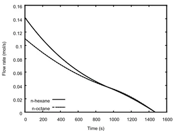
Figure 15 displays the instantaneous leak flow rates of n-hexane and n-octane as a function of time for the initial fluid temperature of 450 K. Because the leak is from the vapor phase, the exit flow rate of n-hexane is larger than that of n-octane at the beginning of the simulation; thus, n-hexane depletes faster. At about 940 s, the flow rates of the two components become equal. After that, until the end of the simulated time, the flow rate of n-octane is larger.
This case illustrates the simulator’s ability of dealing with the change to the number of phases present in the vessel and its effect on the properties of the exiting stream.
Discharge of methane+ethane+propane: comparison with Haque et al.’s (1992b) data
This case considers experiment S9 of Haque et al. (1992b), which used a vertical vessel with torispherical ends and the following dimensions: tangent-to-tangent distance of 2.250 m, internal diameter of 1.130 m, wall thickness of 0.059 m, with a circular orifice whose diameter is 0.010 m, positioned at the top of the vessel. Such a vessel has
an internal volume of 2.50 m3. As torispherical geometry
is unavailable in the current version of our simulator, a vertical cylindrical vessel of the same volume and diameter is assumed, and its corresponding length is 2.49 m. It was also assumed that the vessel is made of stainless steel 316 with mass equal to 5515.2 kg. The vessel is initially charged with a mixture of methane, ethane, and propane, whose mole fractions are equal to 0.855, 0.045, and 0.100, respectively. The initial temperature and total amount in the vessel were taken equal to 303 K and 15060 moles, which give an initial pressure of 120 bar and a mass of 256.6 kg of fluid initially inside the vessel. Therefore, the initial mass of fluid is just 4.4% of the total mass of the system. As in case 4.3, the vessel is considered as adiabatic and the internal energy of the solid is considered in the simulation, with the heat capacity of steel at constant volume given by Eq. (6). The binary interaction parameters of the Peng-Robinson EOS are set equal to zero, which is typical for hydrocarbon mixtures (Reid et al, 1987). The existence of a single vapor phase throughout the simulated period is predicted. Figure 16 compares the experimental (Haque et al., 1992b) pressure with the calculated pressure, the latter plotted against rescaled time, which is the simulation time divided by a coefficient of discharge of 0.57, such that the rescaled time at the end of the run is equal to 1200 seconds. 380
390 400 410 420 430 440 450
0 200 400 600 800 1000 1200 1400 1600
Temperature (K)
Time (s) From vessel at 450 K
From vessel at 460 K
Fig. 14. Temperature at exit point in a vessel loaded with an equimolar n-hexane+n-octane mixture: effect of initial vessel temperature.
0.1 0.2 0.3 0.4 0.5 0.6 0.7 0.8
0 200 400 600 800 1000 1200 1400 1600
Pressure (MPa)
Time (s) From 450 K
From 460 K
Figure 12. Pressure in a vessel loaded with an equimolar n-hexane+n-octane mixture: effect of initial vessel temperature.
380 390 400 410 420 430 440 450 460
0 200 400 600 800 1000 1200 1400 1600
Temperature (K)
Time (s) From 450 K
From 460 K
Despite the similar trends, the calculated pressure is higher than the experimental pressure. According to Haque et al. (1992b), the final experimental temperature of the wall in contact with the gas is about 290 K. They also report the formation of a small volume of liquid phase in the vessel and the final temperature of the solid wall in contact with it is about 250 K. As the simulator adopts a homogeneous equilibrium model, the calculated temperatures of the fluid and of the vessel wall are equal, initially 303 K, and 284.6 K at the end of the simulation, which is somewhat smaller than the final experimental temperature of the wall in contact with the gas (290 K).
CONCLUSIONS
This work presented the results of a simulator based on the homogenous equilibrium assumption for discharges
from pressure vessels that contain non-reactive mixtures. The particular feature of this simulator is that it evaluates all the thermodynamic properties using the same equation of state, including phase equilibrium conditions, calorimetric properties, and derivative properties, such as the sound speed. The Peng-Robinson equation of state was used, but the formulation is general and it is possible to adopt other thermodynamic models.
The conceptual and sensitivity analyses reported here demonstrate that the simulator predicts meaningful trends for the complex phenomena that take place during discharge operations. The simulated results generally agree with the experimental fluid discharge data when a coefficient of discharge is used. Future work on this simulator will focus on: (a) the effect of liquid swelling caused by bubbles due to non-instantaneous phase disengagement during leaks of condensable fluids; (b) expanding the availability of heat transfer models available; (c) studying the venting dynamics of vessels with several runaway reactions.
ACKNOWLEDGEMENTS
A. Basha thanks Itochu Corporation for the support of her M.S. studies at Texas A&M University at Qatar. The authors acknowledge the suggestions of Dr. Valeria Casson-Moreno (University of Bologna, Italy).
NOMENCLATURE
out m
A
orifice area at exit point mv
c
specific heat capacity at constantvolume
dch
h
molar enthalpy of the discharged fluid at the entrance of the hypothetical nozzleout m
h
molar enthalpy at exit point mout m
M
molar mass at exit point mi
n
number of moles of component iin the vessel
out im
n
molar flow rate of component i instream m
out
ns
number of streams that exit the vesselQ
heat transfer to the fluid in the vesseldch
s
molar entropy of the discharged fluid at the entrance of the hypothetical nozzle0 0.02 0.04 0.06 0.08 0.1 0.12 0.14 0.16
0 200 400 600 800 1000 1200 1400 1600
Flow rate (mol/s)
Time (s) n-hexane
n-octane
Fig. 15. Exit flow rate from a vessel loaded with an equimolar
n-hexane+n-octane mixture for initial vessel temperature of 450 K.
0 2 4 6 8 10 12 14
0 200 400 600 800 1000 1200
Pressure (MPa)
Time, rescaled time (s)
Calculated
Experimental
out m
s
molar entropy at exit point mt
timeout m
u
fluid speed at exit point mU
internal energy of the fluid and ofthe vessel wall
out m
v
fluid molar volume at exit point mREFERENCES
Bendiksen, K.H., Maines D., Moe, R. and Nuland, S., The Dynamic Two-Fluid Model OLGA: Theory and Application, SPE Production Engineering,May issue, 171 (1991).
Birch, A.D., Hughes, D.J. and Swaffield, F., Velocity Decay of
High Pressure Jets, Combust. Sci. Technol., 52, 161 (1987). British Stainless Steel Association, http://www.bssa.org.uk/
topics.php?article=139, accessed on June 22 (2016).
Callen, H.B., Thermodynamics and an Introduction to Thermostatistics, 2nd ed., Wiley, New York (1985).
Castier, M., Solution of the Isochoric-Isoenergetic Flash Problem by Direct Entropy Maximization, Fluid Phase Equilib., 276,7 (2009).
Castier, M., Kanes, R. and Véchot, L.N., Flash Calculations with
Specified Entropy and Stagnation Enthalpy, Fluid Phase
Equilib., 408, 196 (2016).
Castier, M., Thermodynamic Speed of Sound in Multiphase Systems, Fluid Phase Equilib., 306, 204 (2011) .
Cumber, P. Predicting Outflow from High Pressure Vessels, Trans
IChemE,79, 13 (2001).
D’Alessandro, V., Giacchetta, G., Leporini, M., Marchetti, B. and Terenzi. A., Modelling Blowdown of Pressure Vessels Containing Two-Phase Hydrocarbons Mixtures with the Partial Phase Equilibrium Approach. Chem. Eng. Sci., 126, 719 (2015).
Espósito, R.O., Castier, M. and Tavares, F.W., Calculations of Thermodynamic Equilibrium in Systems Subject to Gravitational Fields, Chem. Eng. Sci., 55, 3495 (2000). Firoozabadi, A., Thermodynamics of Hydrocarbon Reservoirs,
McGraw-Hill, New York (1999).
Haque, M.A., Richardson, S.M. and Saville, G., Blowdown of Pressure Vessels I. Computer Model, Trans. Inst. Chem. Eng. 70, 3 (1992a).
Haque, M.A., Richardson, S.M., Saville, G., Chamberlain, G. and Shirvill, L., Blowdown of Pressure Vessels II. Experimental Validation of Computer Model and Case Studies, Trans. Inst.
Chem. Eng. 70, 10 (1992b).
Houf, W.G. and Winters, W.S., Simulation of high-pressure liquid hydrogen releases, Int. J. Hydrogen Energy 38, 8092 (2013).
Kanes, R., Basha, A., Véchot, L.N. and Castier, M., Simulation of Venting and Leaks from Pressure Vessels, J. Loss Prev. Proc. Ind., 40, 563 (2016).
Lemmon, E.W., Huber, M.L., McLinden, M.O., NIST Reference Fluid Thermodynamic and Transport Properties-REFPROP, Version 8 User’s Guide, U.S. Department of Commerce Technology Administration, National Institute of Standards and Technology, Standard Reference Data Program, Gaithersburg (2007).
Mahgerefteh, H. and Wong, S.M.A., A Numerical Blowdown Simulation Incorporating Cubic Equations of State, Comput. Chem.Eng.,23, 1309 (1999).
Michelsen, M.L., The Isothermal Flash Problem. Part I. Stability, Fluid Phase Equilib., 9, 1 (1982) .
Peng, D.Y. and Robinson, D.B., A New Two-Constant Equation of State, Ind. Eng. Chem. Fundamentals, 15, 59 (1976). Press, W.H. Flannery, B.P., Teukolsky, S.A. and Vetterling,
W.T., Numerical Recipes in Fortran 77: The Art of Scientific
Computing, Cambridge University Press. Cambridge, UK (1992).
Reid, R.C., Prausnitz, J.M. and Poling, B.E., The Properties of Gases and Liquids, McGraw-Hill, New York (1987).
Renfro, J., Stephenson, G., Marques-Riquelme, E. and Vandu, C. Use Dynamic Models When Designing High-Pressure Vessels. Hydrocarbon Process., May, 71 (2014).
Richardson, S.M. and Saville, G., Blowdown of LPG Pipelines, Process Safety and Environmental Protection,74, 235 (1996).
Speranza, A., Terenzi, A., Blowdown of Hydrocarbons Pressure Vessels with Partial Phase Separation. Applied and Industrial Mathematics in Italy - Series on Advances in Mathematics for
Applied Sciences, 69. World Scientific (2005).
Véchot, L.N., Securité des Procédés. Emballement De Réaction. Dimensionnement des Évents de Sécurité pour Systèmes Gassy ou Hybrides Non Tempérés: Outil, Expériences et Modèle, Ph.D. thesis, École Nationale Supérieure des Mines de Saint-Étienne, France (2006).
Winters, W.S., Modeling Leaks from Liquid Hydrogen Storage Systems, Sandia National Laboratory, Report SAND2009-0035 (2009).
Witlox, H.W.M. and Bowen, P., Flashing Liquid Jets and Two-Phase Dispersion - A Review, Contract 41003600 for HSE, Exxon-Mobil and ICI Eutech, HSE Books, Contract research report 403/2002 (2002).