Optimal Homotopy Asymptotic Method for a thin film flow of a pseudo plastic fluid draining down or lifting up on a cylindrical surface

(1)

www.ache.org.rs/CICEQ

Chemical Industry & Chemical Engineering Quarterly 19 (4) 513−527 (2013) CI&CEQ

M. KAMRAN ALAM1 M.T. RAHIM1 S. ISLAM2 A.M. SIDIQQUI3

Department of Mathematics, National University of Computer &

Emerging Sciences, Peshawar, Pakistan [email protected]

2_{Department of Mathematics,}

Abdul Wali Khan University, Mardan, Pakistan

3_{Pennsylvania State University,}

York Campus, 1031 Edgecombe avenue, York, PA 17403, USA

SCIENTIFIC PAPER

UDC 539.216:532.51:517.93 DOI 10.2298/CICEQ120328086A

_{OPTIMAL HOMOTOPY ASYMPTOTIC}

METHOD FOR A THIN FILM FLOW OF A

PSEUDO-PLASTIC FLUID DRAINING DOWN

OR LIFTING UP ON A CYLINDRICAL

SURFACE

In this study, the pseudo-plastic model is used to obtain a solution for steady thin film flow on the outer surface of a long vertical cylinder for lifting and drainage problems. The non-linear governing equations subject to appropriate boundary conditions are solved analytically for velocity profiles by a modified homotopy perturbation method called the optimal homotopy asymptotic method. Expressions for the velocity profile, volume flux, average velocity, shear stress on the cylinder, normal stress differences, and force to hold the vertical cylindrical surface in position have been derived for both the problems. For the non-Newtonian parameter β = 0, we retrieve Newtonian cases for both the problems. We also plot and discuss the effects of the Stokes number, St,

the non-Newtonian parameter, β, and the thickness, δ, of the the fluid film on the fluid velocities.

Keywords: Lifting and drainage problems, pseudo plastic fluid, optimal homotopy asymptotic method.

Nonlinear evolution equations represent large varieties of physical, chemical, and biological pheno-mena. The exact solutions of these nonlinear equa-tions, if available, facilitate the verification of nume-rical solvers and add in the stability analysis of solu-tions. In nonlinear science, analytical solutions to non-linear partial differential equations play an important role, especially in nonlinear physical science, since they can provide much physical information and more inside into the physical aspects of the problem and thus lead to further applications.

Over the past few decades there has been growing recognition of the fact that many fluids of industrial significance do not obey the Newtonian pos-tulate of linear relationship between the shear stress and shear rate. Therefore, these fluids are known as non-Newtonian fluids. Common examples of such fluids are slurries, pastes, gels, molten plastics and lubricants containing polymer additives. Various food stuffs such as honey and tomato sauce, biological

Correspondence: S. Islam, Department of Mathematics, Abdul Wali Khan University, Mardan, Pakistan.

E-mail: [email protected] Paper received: 28 March, 2012 Paper revised: 16 August, 2012 Paper accepted: 25 September, 2012

fluids like blood and synovial fluid naturally found in cavities of synovial joints also belong to the general class of the non-Newtonian fluids [1,2]. The simplest model of non-Newtonian fluids is the power law model and a special case of the power law equation, with

< 1

n , is the pseudo plastic model. Commonly encountered non-Newtonian fluids like polymer solu-tions, paper pulps, detergents, oils and greases may be classified by the pseudo-plastic fluid model [3]. The pseudo plastic fluids represent shear thinning fluids and, as far as we know, this class of non-New-tonian fluids received less attention in the literature of thin film flow.

(2)

contact with stationary air. Our aim here is to find the effects of the non-Newtonian parameter β on the steady flow of pseudo plastic fluid flowing down on an infinite vertical cylinder.

Recently, thin film flows of non-Newtonian fluids have become an attractive research field for due to their wide applications in nonlinear sciences and engineering industries. Landau et al. [4] discussed the drainage thin film flow of Newtonian fluids. Siddiqui et al. [5] found the results for a drainage problem for thin film flow of a fourth grade fluid down a vertical cylin-der and found the exact solution for the Phan-Thein- -Tanner (PTT) fluid for both lifting and drainage prob-lems [6]. Siddiqui et al. [7] also considered the same flow of non-Newtonian fluids on a moving belt.

The optimal homotopy asymptotic method was first proposed by Marinca and Herisanu in 2008 [10]. It is a modified homotopy perturbation method with the help of the least squares technology [11]. The method was re-named as the optimal homotopy-anal-ysis approach [15].

Recently, Marinca and Herisanu [10-13] intro-duced OHAM for approximate solution of nonlinear problems of thin film flow of a fourth grade fluid down a vertical cylinder. In their work they have used this method to understand the behavior of nonlinear mechanical vibration of electrical machine. They also used the same method for the solution of nonlinear equations arising in the steady state flow of a fourth-grade fluid past a porous plate and for the solution of nonlinear equation arising in heat transfer. Here we use OHAM for the solution of the thin film flow problems and it is observed that OHAM is an easy, flexible and reliable method.

The purpose of this paper is to discuss the non-linear problems of thin film flow on cylindrical surfaces that arise from the mathematical modeling of pseudo plastic fluid In the present paper, we consider the thin film flow of an incompressible, pseudo plastic fluid on the surface of a vertical cylinder for both lifting and drainage problems. To the best of the authors’ know-ledge, no attempt has been made so far to discuss the thin film flow of a pseudo plastic fluid on a cylin-drical surface, and this type of problem is solved by OHAM for the first time.

In this paper, the governing equations, formul-ation of the drainage and lifting problems are deve-loped. The basics of the Optimal Homotopy Asymp-totic method, solution of the problem, average veloci-ties and volume flow rates are given for both the problems, and the obtained results are discussed.

Governing equations

The basic equations governing the motion of an isothermal, homogeneous, incompressible fluid are:

div = 0V (1)

ρD =ρ −grad +div Dt P

V

f S (2)

where ρ is the constant fluid density, V is the velocity vector, f is the body force per unit mass, P denotes the dynamics pressure, Dt denotes the material deri-vative defined as:

(

)

∗ ∂

∗ + ⋅ ∇ ∗ ∂

( )

= ( ) ( ) D

V Dt t

S is the extra stress tensor which for pseudo plastic fluid model is defined as [8]:

(

)(

)

λ ∇ λ µ η

+ 1 + 1− 1 + 0 1

=

2 1 1 1

S S A S SA A (3)

where η0 is the zero shear viscosity, λ1 is the relax-ation time and µ1 is the material constant.

The first Rivlin-Ericksen tensor, A , is defined 1 as:

(

)

+

= (grad ) grad T

1

A V V (4)

The contravariant convected derivative denoted by super imposed ∇ over S is defined as:

{

}

∇

− +

D

= (grad ) (grad ) D

T t

S

S V S S V (5)

It can be noted that if we substitute λ1=µ1= 0 in Eq. (3), we recover the constitutive equation of a Newtonian fluid.

Formulation of the drainage problem

Consider a non-Newtonian, incompressible, lami-nar pseudo-plastic fluid falling on the outside surface of an infinitely long vertical cylinder of radius R, in the form of a thin, uniform axisymmetric film of thickness

δ, in contact with stationary air (Figure 1). The flow is driven through the action of gravity alone and the ambient air is assumed to be stationary.

The flow is assumed to be steady and the sur-face tension of the fluid negligible, and that the pres-sure is atmospheric. In view of the geometry involved we use cylindrical coordinates ( , , )r θ z and consider the r-direction is normal to the cylinder and the z -direction is along the cylinder which is in downward direction. We assume the velocity vector V and the stress tensor S as:

[

]

= 0,0, ( )w r

(3)

= ( )r

S S (7)

The boundary conditions for the problem are:

δ

+

rz= 0 at = (free surface)

S r R (8)

= 0 at = (no slip condition)

w r R (9)

where Srz is the shear stress component of pseudo plastic fluid. By substituting Eq. (6) in Eqs. (1) and (2), the continuity Eq. (1) is identically satisfied and the momentum [2] of Eq. (2) reduces to:

ρ ∂

− + +

∂ 1

1 d 0 = ( )

d rr p

rS f r r r

θ ρ θ ∂ − + + ∂ 2 2 1 1 d

0 = ( )

d r p

r S f

r r r (10)

ρ ∂

− + +

∂ 3

1

0 = p d (rS_rz) f z r dr

where f1, f2 and f3 are components of body force in

r, θ and z directions, respectively.

Figure 1. Geometry of the problem.

Since z coordinate and gravitational force are in the downward direction and pressure is assumed to be atmospheric, the above equations become:

ρ + 1 d

0 = ( ) d rSrz g

r r (11)

Making use of Eqs. (5)–(7) in Eq. (3), we find the non-zero components of S as:

(

)

η λ µ

λ µ   − _ _     + − _ _   2

0 1 1

2 2 2 1 1 d ( ) d = d 1 d rr w r S w r

(

)

η λ µ         + − _ _   0 2 2 2 1 1 d d = = d 1 d rz zr w r S S w r (12)

(

)

η λ µ

λ µ   − _ _   −   + − _ _   2

0 1 1

2 2 2 1 1 d ( ) d = d 1 d zz w r S w r

θ µ1−λ1 θ

1 d = ( ) 2 d z r w S S r

θ λ1+µ1 θ

1 d = ( ) 2 d r z w S S r

On substituting the value of S_rz , Eq. (11) redu-ces to the following form:

(

)

η ρ λ µ   _ _    _ _       ₋   _ _   _ + − _ _ _        0 2 2 2 1 1 d d d = d d 1 d w r r gr r w r (13)

and the boundary conditions (8) and (9) into:

δ

+ d

= 0 at = (free surface) d

w

r R

r (14)

= 0 at = (no slip condition)

w r R (15)

Introducing dimensionless parameters as:

δ δ η δ * * * * 0 0 0 = , = , = , = rz

rz

w r S

U

U R R

The dimensionless form of Eq. (13) and bound-ary conditions (14) and (15) by omitting the “*” become:

β   _ _    _ _       ₋   _ _   _ + _ _ _      2 d d d = d d 1 d t w r r rS r w r (16)

(

+δ

)

d

= 0 at = 1 d

w

r r

= 0 at = 1

w r (17)

where β λ2−µ2 2 δ2

1 1 0

= ( )U / and ρ δ2 η

0 0 = / t

S g U rep-resents the Stokes number. Integrating Eq. (22) once with respect to r and using boundary condition (23), we get:

(

)

(

)

(

)

(

)

β δ δ   − + − _ _   = + − 2 2 ₂ 2 ₂ d d 1 =

d 2 d

1 2

t

w S w

r r

S

r

(4)

= 0 at = 1

w r

or:

(

)

(

+δ 2− 2

)

= 1 2

t rz

S

S r

r (19)

= 0 at = 1 w r

The above Eq. (18) along with one boundary condition is a highly non-linear first order differential equation. It is to be noted that this problem is a well-posed problem but it is difficult to find its exact solution; thus, we use optimal homotopy asymptotic method (OHAM) to solve this problem.

Basic idea of optimal homotopy asymptotic method (OHAM)

In this section, we introduce the basic idea of optimal homotopy asymptotic method (OHAM) [9-11] and solve Eq. (18) using this method.

We apply OHAM to the following differential equation:

+ +

( ) ( ( )) ( ) = 0, ( ) = 0

L w(r) N w r g r B w (20)

where L is a linear operator, r denotes an indepen-dent variable, w r( ) is an unknown function, ( )g r is a known function, N w r( ( )) is a nonlinear operator and

B is a boundary operator. The OHAM now constructs an optimal homotopy ψ( ; ) :r p B×[0,1]→ ℜ which satisfies the following homotopy equation, see for example [9-11].

[

ψ

]

ψ

ψ ψ

− + +

+

(1 ) ( ( , )) ( ) = ( )[ ( ( , )) ( ) ( ( , ))], ( ( , )) = 0

p L r p g r H p L r p

g r N r p B r p (21)

where p∈[0,1] is an embedding parameter, H p( ) is a nonzero auxiliary function for p ≠0 and H(0) = 0,

ψ( ; )r p is an unknown function. Obviously, when = 0

p and p= 1, it holds that:

ψ( ,0) =r w r0( ), ψ( ,1) = ( )r w r (22)

Thus, as p increases from 0 to 1, the solution ψ( , )r p varies from the initial guess w r0( ) to the solution w r( ), where w r0( ) is obtained from equation (21) for p= 0:

+

0 0

( ( )) ( ) = 0, ( ) = 0

L w r g r B w (23)

We choose the auxiliary function H p( ) in the form:

+ 2 +

1 2

( ) = ...

H p pC p C (24)

or we also choose the auxiliary function in the form [12,13]:

τ = τ + 2 τ

1 2

( , ) ( , i) ( , j) H p ph C p h C

where C1,C2,... are auxiliary constants to be deter-mined in an optimal manner.

Next the method expands ψ( ; ;r p C_i) into a Tay-lor’s series about the parameter

p

as follows [10]:

ψ

≥

+



0

1

( , , ) = ( ) ( , ) k, = 1,2,...

i k i

k

r p C w r w r C p i (25)

Convergence of the series (25) depends upon the auxiliary constants C1,C2,... and if it converges at

= 1

p then we have [10]:

ψ ₀ +



=1

( , ) = ( ) ( , ), = 1,2,... M

i k i

k

r C w r w r C i M (26)

Substituting Eq. (25) into Eq. (24) and equating the like powers of p, the original nonlinear problem is converted into a sequence of linear problems. The resulting linear problems can now be solved and their solutions are used to construct an Mth

order solution, which involves C_i , of the original problem through Eq. (26). Then inserting Eq. (24) into Eq. (21) results in the following residual:

+ +

( ) ( )

( , ) = ( m( , )) ( ) ( m( , ))

i i i

R r C L w r C g r N w r C (27)

If R r C( , _i) = 0, for some values of C_i , then ( , )

m i

w r C will coincide with the exact solution. However, this does not happen in general, espe-cially in nonlinear problems. Therefore, optimal values of the auxiliary constants C C1, 2,...,CM are calculated aimed at minimizing the following functional J [10]:



1 2

1 2 ₀ 1 2

( , ,..., n) = ( , , ,..., m)d

J C C C R r C C C r (28)

Thus, the unknown constants C i_i( = 1,2,..., )m

can be optimally identified from the following con-ditions [10]:

∂ ∂ ∂ 1 ∂ 2

= = ... = 0

J J

C C (29)

With these known values of the auxiliary cons-tants, C C1, 2,...,CM, the approximate solution (34) is now well determined.

Solution of the drainage problem by OHAM

(5)

i) Zeroth-order problem

The zeroth-order problem is given by:

(

δ

)

 

+ _ 2− + 2_ 0

d

1 = 0 d 2

t w S

r r

r (30)

subject to boundary condition:

0= 0 at = 1

w r

ii) First-order problem

The first-order problem is defined as follows:

(

)

(

)

{

}

[

]

(

)

δ δ β δ + + − + + − −  _{ } _ − + + _ _{ } + − _  

2 ₂ 2 ₂

1

1 2

2 ₂

0 1 0

1 d

1 1

d 2

dw d

1 1 = 0

dr 2 d

t

t w S

r r C r

r w C S C r r (31)

along with the boundary condition:

1= 0 at = 1

w r

iii) Second-order problem

We introduce the second-order problem:

(

)

(

)

(

)

(

)

(

)

(

)

δ β δ β δ + + − +   + − − +       + _ + − − − _   2 ₂ 2 2 2 ₂ 0 0 2 2 ₂ 0 1 1 1 d 1 d 2 d d 1 1

d 2 d

1 1 = 0

t

w C S

r r

r

w S w

C r

r r r

dw dw

C S r C

dr dr

(32)

2= 0 at = 1

w r

Solving Eqs. (30)-(32) with the corresponding boundary conditions, we obtain the solutions of zeroth-, first- and second-order problems as follows:

i) Zeroth-order solution

The solution of Eq. (30) is given by:

δ   − + +     2 2 0 1

( ) = (1 ) ln 2 2 2

t

S r

w r r (33)

ii) First-order solution

The first order solution is obtained by solving equation (31) along with the boundary condition:

(

)

(

)

(

)

(

)

(

)

β

δ

δ δ δ

− − + − − + + + + 3 6 2 4 1 1 2 4 2 2

( ) = [ 1 { 2 1 32

5 6 2 } 12 1 ln ] t

C S

w r r r

r

r r r

(34)

iii) Second-order solution

Solving Eq. (32) subject to boundary condition, we get the second order solution:

(

)

(

)

(

)

(

)

(

)

β

δ

δ δ δ

− − + −

− + + + + +

3

6

2 2 4

1

2 4

4

2 2

( ) = [6 { 1 { 2 1 192

5 6 2 }} 12 1 ln ] t

S C

w r r r r

r

r r r

(

)

(

)

(

)

(

)

(

)

δ

δ δ δ

+ − − + −

− + + + + +

6

2 2 4

2

4

2 2

6 { 1 ( 2 1

5 6 2 ) 12 1 ln }

r C r r

r r r

(

)

(

)

(

)

(

)

(

)

δ

δ δ δ

+ − − + −

+ + + + + +

6

2 2 2 4

1

4

2 4

[6 1 { 2 1

5 6 2 } 72 1 ln ]

C r r r

r r r

(

)

(

)

(

)

(

)

β δ

δ δ δ

+ − + + −

− + + + − + +

2

10 8

4 8 10

6 2

( 2 15 1

60 1 30 1 3 1 )

r r

(

)

(

)

(

)

(

)

δ δ

δ δ δ δ δ δ

+ + + − +

+ + − + + − + +

2

4_{{20 3} 2 ₂ _{{ 30}

2 30 2 5 2 }}

r

(

δ

)



+ + _



6

4 2

120r 1 lnr St (35)

Substituting Eqs. (33)-(35) into Eq. (26) yields the second-order approximate solution (m= 2) for Eq. (18):

(

)

+ = + + +



(2) 0 =1

0 1 1 2 2

= ( ) ( , ) =

( ) ( , ) , ... m

k i

k

w w r w r C

w r w r C w r C

or, equivalently: δ   − + + +    

(2) 2 2

drainage

1

( ) = (1 ) ln 2 2 2

t S r

w r r

(

)

(

)

(

)

(

)

(

)

β

δ

δ δ δ

+ − − + − − + + + + + 3 6 2 4 1 2 4 2 2

[ 1 { 2 1 32

5 6 2 } 12 1 ln ] t

C S

r r

r

r r r

(

)

(

)

(

)

(

)

(

)

β

δ

δ δ δ

+ − − + −

− + + + + +

3

6

2 2 4

1 4

4

2 2

[6 { 1 { 2 1 192

5 6 2 } 12 1 ln } t

S C

r r r

r

r r r

(

)

(

)

(

)

(

)

(

)

δ

δ δ δ

+ − − + −

− + + + + +

6

2 2 4

2

4

2 2

6 { 1 ( 2 1

5 6 2 ) 12 1 ln }

r C r r

r r r

(

)

(

)

(

)

(

)

(

)

δ

δ δ δ

+ − − + −

− + + + + +

6

2 2 2 4

1

4

2 4

[6 1 { 2 1

5 6 2 } 72 1 ln

C r r r

r r r

(

)

(

)

(

)

(

)

β δ δ

δ δ

+ − + + − + +

+ + − + +

2 4

10 8 6

8 10

2

( 2 15 1 60 1

30 1 3 1

r r r

r

(

)

(

)

(

)

(

)

δ δ

δ δ δ δ δ δ

+ + + − +

+ + − + + − + + +

2

4_{{20 3} 2 ₂ _{{ 30}

2 30 2 5 2 }}

(6)

(

δ

)



+ + _+



6

4 2

120r 1 lnr St ... (36) Here it should be noted that for β= 0 , we get a

solution for a Newtonian fluid [4].

Flow rate and average velocity of thin film flow of drainage problem

The flow rate per unit width is given by:

δ π



1+ (2)

drainage 1

= 2 ( )d

Q rw r r

Substituting Eq. (36) in above equation and then integrating, we obtain the flow rate of pseudo plastic fluids as:

(

)

π δ δ δ  +      + − − + + − + _  _ _  _      2 6

(1 ) 1 1

= 4 ln(1 ) 1 1

2 4 2 4

t S Q

β

δ δ δ

  

+  + _ + + − + _−



3

2 2

1 ₍₁ ₎ 1 _2ln(1 _{) (1} ₎

16 6

t

C S

{

}

δ δ δ

δ δ δ   + + + −  + − +   + + + − −

4 2 2

(1 ) (1 ) (1 ) {48( ln(1 )

4 2 2

5 6 (2 ) 2}

δ δ δ

δ δ δ   − − + + + + +   + + + + + 6 2 1 1

(1 ) (5 6 (2 ))

6 2

(1 )

(5 6 (2 ))] 2

(

)

(

)

{

β β δ

+ 2 2+ + + 2 + +

1 1 2 1

1

6 2 10 ln(1 )

92 St A C C C C S Dt

(

)

(

)

(

)

δ β δ δ  ₊    + + − −      ₊   ₊      − _ − _{ }+ − _     2 2

1 1 5

4 6

6

1 1 6 (1 ){

2 2

1 1 1 1

}

4 4 6 6

t

C S C D

D

(

)

(

)

(

)[

]

δ δ β δ δ  ₊   ₊      + + _ − _− _ − _+     + − + − 6 3

2 2 4 2

1

1 2

1 1 1 1

{15(1 ) 2

6 6 3 3

6 (1 ) 1 t C S D D

(

)

(

)

₍

₎

(

)

δ β δ β δ   ₊ _   − _ − + + +     ₊    + + − +     4 2

7 1 3 1

2 2

1

1 1

(72 (1 ) 4 4

1 1

12 ) 2ln 1 1 }]

4 4

t

D C S D C

C S A

where A D D D D D D, , 1, 2, 3, 5, 6 andD7 are constants which are given in Appendix.

The average velocity, W , is given by:

π +δ 2−

=

[(1 ) 1]

Q W

Normal stress difference

The expressions (12) show that the normal stress difference is given by:

(

)

η λ µ

λ µ   − _ _     − _ _     + − _ _   2

0 1 1

2

2 2

1 1

d 2 ( )

d d

= = 2

d d

1

d

rr zz rz

w

w r

S S S

r w

r

(37)

which, with help of Eqs. (44) and (22), yields:

(

)

{

}

(

)

(

)

δ β δ − − + ×  ×_ − − + × 2 2 2 6 2 2

4 2 2

= 1

16

8 2 1

t rr zz

t S

S S r

r

r S r r

(

)

(

)

β

(

δ

)



× 3 + + + 2 2 5 2− + 2 4_

1 2 1 2 1 1

t t

S C C C C S r (38) The expression (38) reveals that the normal stress difference vanishes at the free surface

δ

+ = 1

r .

The shear stress on the cylinder

The expression for the shear stress on the vertical cylindrical surface is:

(

)

(

)

{

(

)

}

(

)

(

)

(

)

(

)

(

)

δ δ βδ δ βδ δ

β δ δ βδ δ β δ δ

  + _ + + − + − + − + + _     + + − + + + + +     2 2

2 2 2 2

2 1 1

=1 ₃ ₅ 2

3 3 2 5 2 5

1 1 2 1

2 8 2 2 4 2 2

| =

1

16 1 8 2 2 2 2 2

256

t t t

rz r

t t t

S S C C C S

S

S C C C S C S

Force to hold the vertical cylindrical surface in Position

The force F per unit width to hold the vertical cylinder surface in position can also be determined using the expression for shear stress at the cylinder surface:

(

)



=1 1 = d H rz r F S r

W (39)

(7)

(

− +δ 2

)

− = 1 (1 ) (1 )

2 t F S

H

W (40)

Equation (40) can also be used to determine the length H of the vertical cylinder, once the force per unit width is known.

In the following section, we revisit the lifting problem of the same fluid on an infinite vertical cylin-der.

Lifting problem for the pseudo-plastic fluid

We consider a container filled with an incom-pressible non-Newtonian (pseudo-plastic) fluid as shown in Figure 2. Through this container, a cylinder moves vertically upward with a constant speed U0. The cylinder picks up a thin film fluid of uniform thickness δ. The gravity tries to make the fluid drain down the cylinder.

Figure 2. Geometry of the problem.

The governing Eqs (1) and (2), after using Eq. (6) become:

ρ − 1 d

0 = ( ) d rSrz g

r r (41)

Using the expression for Srz from Eq. (17), we get:

(

)

η

ρ

λ µ

  _ _ 

  _ _ 

 

  

  _ _ 

 _ + − _ _ _

    

 

0

2

2 2

1 1

d

d d

=

d d

1

d

w r

r gr

r _w

r

(42)

and the boundary conditions (8) and (9) into:

δ + d

= 0 at = (free surface) d

w

r R r

0

= at = (no slip condition)

w U r R

The dimensionless form of Eq. (42) and bound-ary condition by omitting the , ,* become:

β

  _ _ 

  _ _ 

 

  

  _ _ 

 _ + _ _ _

    

 

2 d

d d

=

d d

1

t

w r

r rS

r w

dr

(43)

(

+δ

)

d

= 0 at = 1 d

w

r r

0

= at = 1

w U r

where 2 2 2 2

1 1 0

= ( )U /

β λ −µ δ and 2 0 0 = / t

S ρ δg ηU rep-resents the Stokes number. Integrating once equation (43) with respect to r and using the boundary condit-ion, we get:

(

)

(

)

(

)

(

)

2 2

2

2 2

d d

1 =

d 2 d

1 2

t

w S w

r r

S r

β δ

δ

 

− − + _ _

 

= − +

(44)

0

= at = 1

w U r

or:

(

)

(

2 2

)

= 1

2 t rz

S S r

r − +δ

0

= at = 1

w U r

Equation (44) along with one boundary condition is a highly non-linear first order differential equation. It is to be noted that this problem is a well-posed problem but it is difficult to find its exact solution; thus, we use the optimal homotopy asymptotic method (OHAM) [10-12] for the solution.

i) Zeroth-order problem

The zeroth-order problem is given by:

(

)

2 2

0 d

1 = 0 d 2

t w S

r r

r +  +δ −  (45) subject to boundary condition:

0= 0 at = 1

w U r

ii) First-order problem

(8)

(

)

(

)

[

]

(

)

2 2 2 2 1 1 2 2 2

0 1 0

1 d

{ 1 1 }

d 2 d

1 1 = 0

d 2

t

t w S

r r C r

r

w C S dw

C r r dr δ δ β δ + − + + − + −  _{ } _ − + + _ _{ } − + _   (46)

1= 0 at = 1

w r

iii) Second-order problem

We introduce the second order problem:

(

)

(

)

(

)

(

)

2

2 0 0 2

2 2

2

2 ₁ ₀ ₂

1 2

1

d d

d

1 [ (

d 2 d 2 d

d d

1 ) 1] [ (

d d

1 ) 1] = 0

t t

t

w w

w C S S

r r C r

r r r r

w w

C S r

r r C β δ δ β δ + − + + − − + − + − − + − − (47)

2= 0 at = 1

w r

i) Zeroth-order solution

The solution of Eq. (45) is given by:

2

2 0

1

( ) = 1 (1 ) ln 2 2 2

t

S r

w r +  − − +δ r

  (48)

ii) First-order solution

The first order solution is obtained by solving Eq. (46) along with the boundary condition:

(

)

(

)

(

)

(

)

(

)

3 6 2 4 1 1 2 4 2 2

( ) = [ 1 { 2 1 32

5 6 2 } 12 1 ln ] t

C S

w r r r

r

r r r

β

δ

δ δ δ

− − − + −

− + + + +

(49)

iii) Second-order solution

Solving Eq. (47) subject to boundary condition, we get the second order solution:

(

)

(

)

(

)

(

)

(

)

3

6

2 2 4

1

2 4

4

2 2

( ) = [ 6 { 1 ( 2 1 192

5 6 2 ) 12 1 ln } t

S C

w r r r r

r

r r r

β

δ

δ δ δ

− − − + − − + + + +

(

)

(

)

(

)

(

)

(

)

6

2 2 4

2

4

2 2

6 { 1 ( 2 1

5 6 2 ) 12 1 ln }

r C r r

r r r

δ

δ δ δ

− − − + − − + + + +

(

)

(

)

(

)

(

)

(

)

6

2 2 2 4

1

4

2 4

[ 6 1 { 2 1

5 6 2 } 72 1 ln

C r r r

r r r

δ

δ δ δ

+ − − − + −

− + + − +

(

)

(

)

(

)

(

)

2 4

10 8 6

8 10

2

(2 15 1 60 1

30 1 3 1

r r r

r

β δ δ

δ δ + − + + + − − + + +

(

)

(

)

(

)

(

)

2

4_{{ 20 3} 2 ₂ _{{ 30}

2 30 2 5 2 }}

r δ δ

δ δ δ δ δ δ

+ − − + − +

+ − + + − + +

(

)

6

)

4 2

120r 1 δ lnr St 

− + _

 (50)

Inserting the values from Eqs. (48)-(50) in Eq. (26), the solution of the differential Eq. (44) at m= 2 takes the form:

(2) 0

=1

0 1 1 2 2

= ( ) ( , ) =

( ) ( , ) ( , ) ,... m

k i

k

w w r w r C

w r w r C w r C

+ = + + +



 or, equivalently:

(

)

2 2 (2) lifting 1

( ) = 1 1 ln 2 2 2

t S r

w r + _ − − +δ r_

  

(

)

(

)

(

)

(

)

(

)

3 6 2 4 1 2 4 2 2

[ 1 { 2 1 32

5 6 2 } 12 1 ln ] t

C S

r r

r

r r r

β

δ

δ δ δ

− − − + − − + + + + +

(

)

(

)

(

)

(

)

(

)

3 6

2 2 4

1 4

4

2 2

[ 6 { 1 ( 2 1 192

5 6 2 ) 12 1 ln } t

S C

r r r

r

r r r

β

δ

δ δ δ

+ − − − + − − + + + + −

(

)

(

)

(

)

(

)

(

)

6

2 2 4

2

4

2 2

6 { 1 ( 2 1

5 6 2 ) 12 1 ln }

r C r r

r r r

δ

δ δ δ

− − − + − − + + + + +

(

)

(

)

(

)

(

)

(

)

6

2 2 2 4

1

4

2 4

[ 6 1 { 2 1

5 6 2 } 72 1 ln

C r r r

r r r

δ

δ δ δ

+ − − − + −

− + + − + +

(

)

(

)

(

)

(

)

2 4

10 8 6

8 10

2

(2 15 1 60 1

30 1 3 1

r r r

r

β δ δ

δ δ + − + + + − − + + + +

(

)

(

)

(

)

(

)

2

4_{{ 20 3} 2 ₂ _{{ 30}

2 30 2 5 2 }}

r δ δ

δ δ δ δ δ δ

+ − − + − +

+ + − + + − + + −

(

)

6

)

4 2

120r 1 δ lnr St  ...

− + _+

 (51)

Here it should be noted that for β= 0, we get a solution for a Newtonian fluid for the lifting case.

Flow rate and average velocity of thin film flow of drainage problem

The flow rate per unit width is given by:

1 (2) lifting 1

= 2 ( )d

(9)

Substituting Eq. (51) in Eq. (52) and then integ-rating, we obtain the flow rate of pseudo plastic fluids as:

(

)

2

6 (1 ) 1

=

2 2

(1 ) 1 1

4 ln(1 ) 1 1

2 4 2 4

t Q S δ π δ δ δ  +  − +      +      + __  _ + − _+ + − − _−      3 2 2

1 ₍₁ ₎ 1 _2ln(1 _{) (1} ₎

16 6

t

C S

β

δ δ δ

   −  + _ + + − + _− 

{

}

4 2 2

(1 ) (1 )

{48{ (ln(1 )

4 2

(1 )

) 5 6 (2 ) 2}} 2 δ δ δ δ δ δ + + − + − + − + + + − + 6 2 1 1

(1 ) (5 6 (2 ))

6 2

(1 )

(5 6 (2 ))] 2

δ δ δ

δ δ δ   + − + + + + +   + + + + +

(

)

2 2

1 1 2

2 1 1

{6 (2 92

10 )ln(1 ) t

t

S A C C C

C S D

β β δ + + + + + + −

(

)

(

)

(

)

2 2

1 1 5

4 6

6

1 1 6 (1 ){

2 2

1 1 1 1

}

4 4 6 6

t

C S C D

D δ β δ δ  ₊    − + − −      ₊   ₊      − _ − _{ }+ − _ −    

(

)

(

)

₍

)[

]

6

2 2 4 2

1 3 1 2 1 1 {15(1 ) 6 6 1 1

2 6 (1 ) 1

3 3 t C S D D δ β δ δ δ  ₊    − + _ − _−    ₊    − _ − _+ − + −  

(

)

(

)

₍

₎

(

)

4 2

7 1 3 1

2 2

1

1 1

(72 (1 ) 4 4

1 1

12 ) 2ln 1 1 }]

4 4

t

D C S D C

C S A

δ β δ β δ   ₊ _   + _ − + + +     ₊    + _ + − + _  

The average velocity, W , is given by:

2 =

[(1 ) 1]

Q W

π +δ −

Normal stress difference

The expressions (14)–(16) show that the normal stress difference is given by:

2 d (1 ) = 2

d rr zz

w

S S r

r r δ  +    − _ __ − _    or:

(

)

(

)

2 2 2 (1 ) = [192 192

48 1 2 1 ln t

rr zz

t

S

S S r r

r

r r S

δ δ  +  −  −  +   + − − + −

(

)

(

)

3 6 2 4 2 2

6 {( 1)( 2 1

5 6 (2 ) ) t S r r r r β δ δ δ − − − + − − + + +

(

)

4

(

)

2

1 1 2

12r 1 δ ln }r C 2 C C

+ + + + +

(

)

(

)

5

2

2 10 8

4

6 2 8

{2 15 1

60 1 30 (1 ) t S r r r r r β δ δ δ + − + + + + − +

(

)

10 4 2

(

) {

2

3 1 δ r  20 3δ 2 δ 30 δ(2 δ) + + + _− − + − + +

(

)

4

(

)

6 2

1 ( 30− +δ(2+δ) − +5 δ(2+δ) )}] 120− r 1+δ ln }r C ]

The above expression reveals that the normal stress difference vanishes at the free surface

= 1

r +δ.

Shear stress on the vertical cylinder

The shear stress on the vertical cylindrical sur-face is:

(

)

(

)

(

)

(

)

(

)

(

)

(

)

(

)

(

)

2 2 2 =1 2 2 2 2 1 1 3 3 1 1 5

3 2 5 2 5 2

2 1

| = 2 [8 2 { 2

4 2 2 }] /

/16(1 {8 2 2 2 ( 2 256

) 2 } )

rz r t t

t

t t

S S S C

C C S

S C C

C S C S

δ δ β δ δ

βδ δ

β

δ δ βδ δ

β δ δ

− + + + − +

+ − + − + +

+ + − + + +

+ + +

Force to hold the vertical cylindrical surface in position

The force F per unit width to hold the vertical cylinder in position can also be determined using the expression for shear stress at the cylinder surface:

(

)

=1 1 = d H rz r F S r

W



(53)

where H is the length of the cylinder. Using Eqs. (6) and (53), we obtain:

(

2

)

= (1 ) 1 (1 ) 2

t F S

H

(10)

Equation (54) can also be used to determine the length H of the cylinder, once the force per unit width is known.

DISCUSSION OF RESULTS

The graphs for the fluid velocities w(2)drainage( )r and w(2)lifting( )r against r are plotted for both drainage and lifting problems various values of Stokes number

t

S , the non-Newtonian parameter β and the thickness

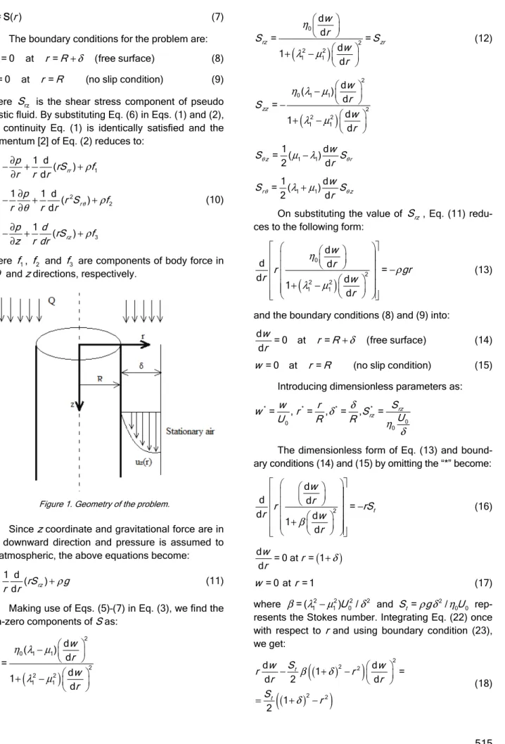
δ of the fluid film respectively, by selecting different values of the auxiliary constants C1 and C2. From Figure 3a, b and c, it is found that the Stokes number

t

S , the non-Newtonian parameter β and the thickness

δ of the fluid film have a direct correlation with the fluid velocity for the drainage case by taking the auxiliary constants C₁= 1.4084694− and C2 = = 0.0976192− .

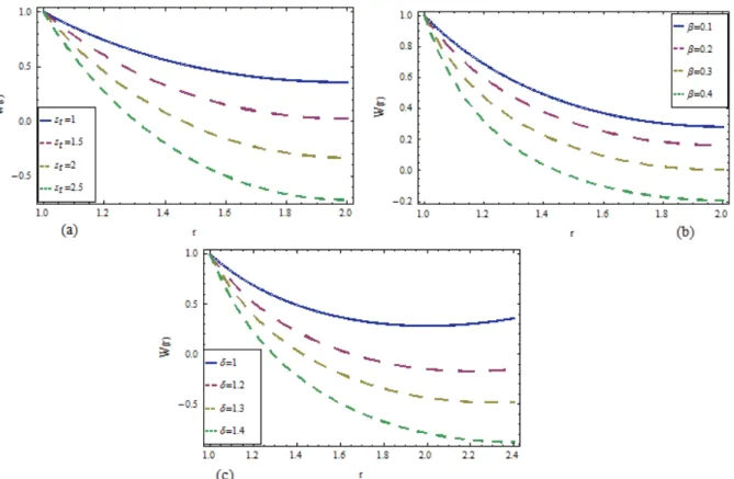
In the lifting case, for the same values of auxiliary constants C1= 1.036774 and C2 =

4.147522

= − , an inverse relation observed for the significant parameters S_t, β and δ in Figure 4a, b and c, respectively. The fluid velocity w r ( ) versus the r -axis for drainage and lifting problems are shown here, plotted for different parameters. For the drainage case

in Figure 5a-c, it is observed that the fluid velocity increases by varying the values of St, β and δ for dif-ferent values of C1= 1.036767 and− C2= 0.000449− . Similarly, for the lifting problem in Figure 6a-c, it is found that the velocity of the pseudo plastic fluid decreases by increasing the values of involved para-meters S_t, β and δ by taking C1= 1.036774 and

2 4.147522

C = − . In the same way, by considering Figure 7a-c for the drainage problem, it is found that the velocity of the fluid increases for the Stokes number S_t, the non-Newtonian parameter β and for the thickness δ of the fluid film by taking the auxiliary constants C1= 1.408469 and− C2= 0.097619− , while in the lifting problem, Figure 8a-c, the fluid velocity decreases for the S_t, β and δ by taking

1= 1.036774

C and C2= −4.147522 . It is also obser-ved that, in Figure 9 for the non-Newtonian parameter

= 0

β , we get the graphs of Newtonian fluids for both the problems. In Table 1, the absolute difference shows the non-Newtonian effect on the velocity profile for the values:

1 2

= 1; = 0.01; = 1; = 1.4084694;

= 0.09761926 t

S C C

β δ

− −

Figure 3. The effect of: a) Stokes number S , b) non-Newtonian parameter t β and c) thickness δ on the dimensionless velocity profile (2)

drainage( )

(11)

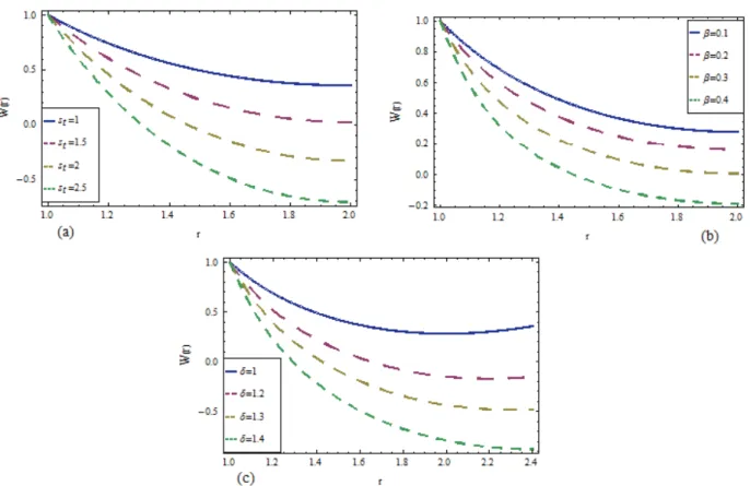
Figure 4. The effect of: a) Stokes number S , b) non-Newtonian parameter t β and c) thickness δ on the dimensionless velocity profile

(2) lifting( )

w r by taking the constants C₁= 1.4084694− and C₂= 0.0976192− .

Figure 5. The effect of: a) Stokes number S , b) non-Newtonian parameter t β and c) thickness δ on the dimensionless velocity profile for

(12)

the lifting problem by taking the constants C₁= 1.0367670− and C₂= 0.0004492.−

(13)

the lifting problem by taking the constants C₁= 1.0467774and C₂= 4.1877176− .

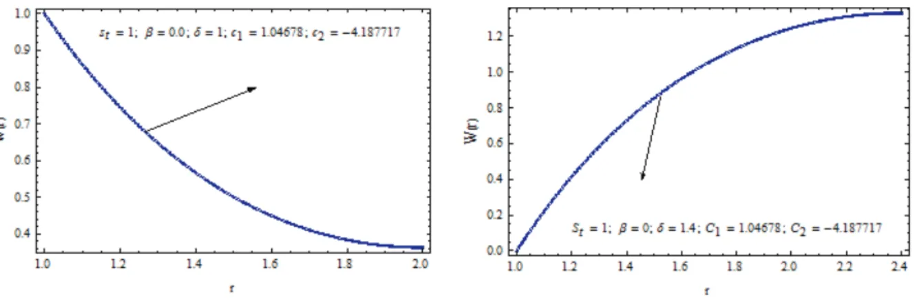
Figure 9. The Newtonian behavior of the fluid velocity for the lifting and drainage cases by taking

1 2

= 1; = 1.4; = 1.04678; = 4.18772

t

S δ C C − and the non-Newtonian parameter β= 0.

Table1. Values for the velocity profile in the drainage case for the viscous (Newtonian) case when

1 2

= 1; = 0.01; = 1; = 1.4084694 = 0.0976192

t

S β δ C − and C −

r 4th-order approximation Exact (drainage) Absolute difference

1.0 0.000000 0.00000 0.00000000

1.1 0.140882 0.13812 0.00276207

1.2 0.259045 0.254643 0.00440172

1.3 0.357586 0.352229 0.00535722

1.4 0.43884 0.432944 0.00589517

1.5 0.504612 0.49843 0.00618175

(14)

Table1. Continued

1.7 0.595138 0.588757 0.00638165

1.8 0.621975 0.615573 0.00640183

1.9 0.637614 0.631208 0.0064061

2.0 0.642701 0.636294 0.00640637

CONCLUSION

In this work, we have used optimal homotopy asymptotic Method proposed by Marinca to find the solution of the flow problem governed by Eqs. (18) and (44). The non-linear governing equations subject to appropriate boundary conditions are solved anal-ytically for velocity profiles by the newly introduced optimal homotopy asymptotic method (OHAM). Expli-cit expressions for the veloExpli-city profile, volume flux, average velocity, shear stress on the cylinder, normal stress differences, and force to hold the cylindrical surface in position are obtained for both the problems. The graphical representations of the velocity profiles of lifting and drainage problems were presented as well.

In this study, all the results obtained from OHAM are logically good and converge to the exact solution as the constant C s_i' increases in the auxiliary func-tion. This method provides us a suitable way to con-trol the convergence of the series solution using the auxiliary constants (C s_i' ) which are optimally deter-mined. We hope that this method has a great poten-tial to help researchers, scientists and engineers of several field to develop a new non-linear analytical technique in the absence of small or large parame-ters.

Appendix

2 3 4 5 6

= 1 6 15 20 15 6 A + δ+ δ + δ + δ + δ +δ

2 3 4 5 6 7 8

= 1 8 28 56 70 56 28 8

D + δ+ δ + δ + δ + δ + δ + δ +δ

(

)

(

)

(

)

(

)

4

1= 40 3 [ 470 { 30

270 40 3 8 10 }]

D δ δ δ

δ δ δ δ δ

− + − + − +

+ − + + + +

(

)

(

)

(

)

(

)

3

2= 3[360 {10 (45

12 8 210 120 45 (10 ) )}]

D δ δ δ

δ δ δ δ δ

+ + +

+ + + + + +

2 3 4

3= 1 4 6 4

D + δ+ δ + δ +δ

(

)

2 2 3

5= 3 24 40 30 12 2

D −δ + δ+ δ + δ +

(

)

2 6= 6 1

D +δ

(

)

(

)

7= 60 2 2 2

D δ +δ +δ +δ

REFERENCES

[1] G. Astarita, G. Marrucci, Principles of Non-Newtonian Fluid Mechanics, McGraw-Hill, London, 1974

[2] R.B. Bird, R.C. Armstrong, O. Hassager, Dynamics of Polymeric Liquids, Fluid Dynamics, Wiley, New York, 1987

[3] M. Moradi, Iranian J. Chem. Eng. 3 (2006) 13-19 [4] L.D. Landau, E.M. Lifshitz, Fluid Mechanics, Second ed.,

Pergamon, New York, 1989

[5] A.M. Siddiqui, R. Mahmood, Q.K. Ghori. Physics Lett., A 352 (2006) 404-410

[6] A.M. Siddiqui, R. Mahmood, Q.K. Ghori. Physics Lett., A 356 (2006) 353-356

[7] A.M. Siddiqui, R. Mahmood, Q.K. Ghori. Chaos, Solitons Fractals 33 (2007) 1006-1016

[8] J.A. Deiber, A.S.M. Santa Cruz, Lat. Am. J. Chem. Eng. Appl. Chem.14 (1984) 19-38

[9] N. Herişanu, V. Marinca, T. Dordea, G. Madescu, Proce-edings of the Romanian Academy, Vol. 9, 2008, pp. 229- -236

[10] V. Marinca, N. Herisanu, I. Nemes. Central European J. Physics 6 (2008) 648- 653

[11] V. Marinca, N. Herişanu, Comput. Mathematics Appl. 61 (2011) 2019–2024

[12] V. Marinca, N. Herisanu, C. Bota, B. Marinca, Appl. Mathematics Lett. 22 (2009) 245-251

[13] N. Herişanu, V. Marinca. Meccanica 45 (2010) 847–855 [14] N. Herişanu, V. Marinca. Comput. Mathematics Appl. 60

(2010) 1607-1615

(15)

M. KAMRAN ALAM1 M. T. RAHIM1 S. ISLAM2 A. M. SIDIQQUI3

Department of Mathematics, National University of Computer & Emerging Sciences, Peshawar, Pakistan [email protected]

2

Department of Mathematics, Abdul Wali Khan University, Mardan, Pakistan

3

Pennsylvania State University, York Campus, 1031 Edgecombe avenue, York, PA 17403, USA

NAUČNI RAD

_{OPTIMALNA HOMOTOPSKA ASIMPTOTSKA}

METODA ZA STRUJANJE PSEUDO PLASTI

Č

NOG

FLUIDA U TANKOM FILMU NIZ ILI UZ CILINDRI

Č

NU

POVRŠINU

U radu je korišćen model pseudo-plastičnog fluida da bi se dobilo rešenje za stacionarno strujanje naviše ili naniže u tankom filmu na spoljnoj površini dugačkog cilindra. Analitičkim rešenjem nelinearnih jednačina, uz primenu odgovarajućih graničnih uslova, pomoću modifikovane metode homotopske perturbacije, nazvane optimalna homotopska asimp-totska metoda, određeni su profili brzine strujanja. Izvedeni su izrazi za profil brzine, zapreminski fluks, srednju brzinu, napon smicanja na cilindru, razlike normalnih napona, silu na vertikalnu cilindričnu površinu za oba slučaja strujanja. Za nenjutnovski parameter razmatrana su strujanja njutnovskog fluida u oba slučaja. Takođe, grački prikazi su isko-rišćeni za razmatranje uticaja Stokes-ovog broja, nenjutnovskog parametra I debljine sloja fluida na brzinu strujanja fluida.