Contents lists available atScienceDirect
Computers, Environment and Urban Systems
journal homepage:www.elsevier.com/locate/ceusA data science approach for spatiotemporal modelling of low and resident
air pollution in Madrid (Spain): Implications for epidemiological studies
Álvaro Gómez-Losada
a,⁎, Francisca M. Santos
b, Karina Gibert
c, José C.M. Pires
baEuropean Commission, Joint Research Centre (JRC), Seville, Spain
bLaboratório de Engenharia de Processos, Ambiente, Biotecnologia e Energia (LEPABE), Departamento de Engenharía Qum´ ica, Faculdade de Engenharia, Universidade do
Porto, Rua Dr. Roberto Frias, Porto 4200-465, Portugal
cKnowledge Engineering and Machine Learning group at Intelligent Data Science and Artificial Intelligence Research Center, Department of Statistics and Operations
Research, Research Institute on Science and Technology for Sustainability, Universitat Politècnica de Catalunya-BarcelonaTech, C/ Jordi Girona 1-3, Barcelona 08034, Spain
A R T I C L E I N F O Keywords:
Air pollution exposure Background pollution levels Hidden Markov Models Inverse distance weighting Ordinary kriging
A B S T R A C T
Model developments to assess different air pollution exposures within cities are still a key challenge in en-vironmental epidemiology. Background air pollution is a long-term resident and low-level concentration pol-lution difficult to quantify, and to which population is chronically exposed. In this study, hourly time series of four key air pollutants were analysed using Hidden Markov Models to estimate the exposure to background pollution in Madrid, from 2001 to 2017. Using these estimates, its spatial distribution was later analysed after combining the interpolation results of ordinary kriging and inverse distance weighting. The ratio of ambient to background pollution differs according to the pollutant studied but is estimated to be on average about six to one. This methodology is proposed not only to describe the temporal and spatial variability of this complex exposure, but also to be used as input in new modelling approaches of air pollution in urban areas.
1. Introduction
Air pollution is a major environmental concern in urban areas worldwide, with significant impacts on societal health and economy (WHO, 2016). There is a growing evidence of mortality and morbidity effects related to long-term exposure to ambient air pollution (Cheng et al., 2017;Lao et al., 2018;Lee, Kim, & Lee, 2014;Weinmayer et al., 2015). Moreover, health outcomes have been seen at very low levels of exposure (Lepeule et al., 2014), and it is unclear whether a threshold concentration exists below which no effects on health are likely. The association among low and long-term air pollution with human health outcomes has not been firmly established and additional insights are needed to collectively strengthening epidemiological evidences. Iden-tify exposures that contribute to health outcomes and construction of exposure summary measures are questions of interest in environmental epidemiology (Weisskopf, Seals, & Webster, 2018), and represent the main motivation of this work.
Background concentration has been defined as the concentration that is not affected by local sources of pollution (Menichini, Iacovella, Monfredini, & Turrio-Baldassarri, 2007;WHO, 1980). In urban areas, the background concentration levels are typically measured at air
pollution monitoring sites far from local sources of pollution (back-ground sites), and these concentrations are considered be the sum of contributions from regional and urban background emissions (Gao et al., 2018). Typically, these background levels are studied: (i) to better understand the contributions of local sources to total pollutant con-centrations; and (ii) to allow the assessment of new pollutant sources that are introduced into the area of study and their impact on local air quality. In this work, this definition of background concentration is extended and it is considered to be influenced by local contributions (e.g., traffic hot-spots). Thus, it is possible to assess a more realistic long-term air pollution exposure of low concentration to which the population is chronically exposed. The importance of its study resides in representing at study areas a range of minimum and stable con-centrations of ambient air pollution, which is permanently resident in the long run.
Opportunities for exploring novel exposures parameters that have been previously difficult to quantify is a key challenge in environmental epidemiology (Tonne et al., 2017). This study aims to provide a reliable estimate of background (low) and long-term air pollution focusing on intra-urban scales, and therefore, to contribute with new input in-formation to epidemiological studies regarding the association of air
https://doi.org/10.1016/j.compenvurbsys.2018.12.005
Received 31 August 2018; Received in revised form 15 November 2018; Accepted 17 December 2018 ⁎Corresponding author.
E-mail addresses:alvaro.gomez-losada@ec.europa.eu,alvaro.gomez.losada@gmail.com(Á. Gómez-Losada).
Computers, Environment and Urban Systems 75 (2019) 1–11
Available online 24 December 2018
0198-9715/ © 2018 The Authors. Published by Elsevier Ltd. This is an open access article under the CC BY license (http://creativecommons.org/licenses/BY/4.0/).
pollution with human health effects in cities. Specific objectives are: (i) to characterize quantitatively the background air pollution (NO2, O3, PM10and SO2) at temporal and spatial scales in Madrid urban area during the period from 2001 to 2017; and (ii) to standardize a robust methodology to estimate a chronic exposure measurement to these air pollutants (or others) and possibly extended to other types of pollution (e.g., noise or odour pollution).
2. Data and methods 2.1. Area of study
Madrid is the third most populous city in the European Union after London and Berlin and the largest city of Spain, with an estimated population of 3.1 million people in the city and 7.3 including the me-tropolitan area (INE, 2017; Madrid City Council, 2017). Madrid's economy is based on the service, construction and industry sectors. Its location in the centre of the country also makes Madrid the main transport knot within the Iberian Peninsula (Cuevas et al., 2014) with road traffic the main source of PM10 and NO2emissions (Montero & Fernández-Avilés, 2018). Quantitatively, 48% of PM10has been proved to be contributed by vehicle emissions (Salvador, Artíñano, Alonso, Querol, & Alastuey, 2004), and NO2and CO are related to traffic in more than 80% (Monzón & Guerrero, 2004). The SO2levels, mainly produced by energy production and distribution activities, and to a lesser extent by the commercial, institutional and households sector, have experienced a decreasing due both to the reduction of residential coal burning and the use of gasoline vehicles, but also by the im-plementation of particlesfilters in diesel engines (Salvador, Artíñano, Viana, Alastuey, & Querol, 2012). As in many urban environments, O3 is photochemically produced (secondary air pollutant) under specific conditions or transported from other regions, presenting higher levels at city outskirts (due to lower levels of nitrogen oxides). In particular in Madrid, 65% of tropospheric O3formation is accounted for traffic-re-lated precursors (Valverde, Pay, & Baldasano, 2016). European Com-mission limits (Directive 2008/50/EC) and WHO guidelines (WHO, 2005) values are currently being complied in Madrid concerning par-ticulate matter, but not for NO2(MAPAM, 2017) with high pollution episodes recently studied (Borge et al., 2018). Although NO2and PM10 ambient air concentrations have shown a clear decreasing trend during the last years due to the emission reductions in the road traffic sector (economic recession from 2008), use of adoptions of eco-friendly fuels (Euro 4 and Euro 5 emission standards in vehicles) and emission control policies, this urban area has experienced an increase of ambient air O3 levels (30–40%,Saiz-López et al., 2017), as well as in other European cities. Unfortunately, air quality in Madrid is still an issue of remarkable concern and therefore motivated to be the focus of this study. 2.2. Data
The air quality monitoring network (AQMN) of Madrid included 24 operating sites in 2017 and is managed by the Madrid City Council, which ensures its correct maintenance and validation of monitored data. These sites are classified according to their location (U-urban, S-Suburban) and main pollution source (T-traffic, B-Background). Location and typology of studied sites are provided in Supplementary Material (SM.– 1). Analysed data in this study were hourly time series (TS) for each year from 2001 to 2017, of NO2, O3, PM10and SO2 ob-tained from 38 monitoring stations (Fig. 1) when available.
Validated hourly data (inμg·m−3) were obtained from the Madrid City Council's Open Data portal (https://datos.madrid.es). Every TS for a given year and air pollutant was studied only if two criteria were met: (i) at least 80% of hourly values were available during the year (minimum of 7008 hourly values); and (ii) at least 11 months should present the mentioned minimum monitoring efficiency (minimum of 576 hourly values). The length of the studied TS differentiated by
monitoring site, year and air pollutant is provided in SM.2. 2.3. Background pollution estimation
Air pollution levels at urban regions depend on the atmospheric phenomena that occur at different spatial scales, from international scales to street levels. Moreover, the choice of the model is dependent on the purpose of the simulation (Borge et al., 2014). In this study, the background air pollution concentration was estimated independently on annual TS of NO2, O3, PM10and SO2pollutants at hourly resolution and summarized as an annual average concentration, using Hidden Markov Models (HMM). These models allow for estimating the back-ground ambient pollution, which represents a long time exposure to air pollution experienced by the population. The methodology for this es-timation has been previously described byGómez-Losada, Pires, and Pino-Mejías (2016)and proved to be a convenient approach for that purpose inGómez-Losada, Pires, and Pino-Mejías (2018). In the interest of space, the elements and a mathematical description of HMM are provided in SM.3. This study represents an application of such metho-dology to Madrid’ urban and metropolitan areas and succinctly ex-plained next.
In this study, the goal of HMM is to obtain groups of hourly ob-servations of air pollutants in each annual TS, forming different clus-ters. These clusters group similar hourly concentration values, which are simultaneously dissimilar to the rest of hourly concentrations grouped in other clusters detected in TS. There are multiple techniques to identify cluster in data. However, the main difference of HMM with the rest of these techniques is that HMM is especially devoted to deal with dependent (TS) data (Zucchini & MacDonald, 2009). Hence, hourly TS observations forming clusters in each TS are assumed to re-present profiles (regimes) of pollution. The more suitable number of clusters detected in each TS is estimated according to the Bayesian in-formation criteria (BIC) value. Each of these pollution profiles may be summarized by its average value, which are calculated as the average values of the hourly observations grouped within each cluster. There-fore, the cluster with lowest average value can be assumed to represent the annual background average concentration of the studied air pollu-tant, and is the one of interest in this work. Likewise, without applying Fig. 1. Studied air quality monitoring sites in Madrid, from 2001 to 2017.
a clustering to the hourly TS observations, the annual average con-centration of all the TS observations provides the average ambient pollution.Fig. 2illustrates the results (in red) after applying the HMM methodology to TS data for estimating the background pollution.
The computational implementation of HMM was performed using the depmixS4 package (Visser & Speekenbrink, 2010) in R software (R Core Team, 2017) and an example script for HMM implementation is provided in SM.4.
2.4. Spatial analysis of background air pollution
After applying independently HMM to each analysed TS (from every available air pollutant, at monitoring sites and by years), the estimated average background air pollution concentrations at sites were used to map the geographical variation of background air pollution over Madrid. According toLi and Heap (2014), spatial interpolation methods fall into three categories: (i) non-geostatistical, (ii) geostatistical; and (iii) combined methods of the previous ones. The selection of an ap-propriate interpolation method for a given input data set is still a key issue on which little guidance exists. In interpolation methods com-monly used in environmental studies, important factors affecting the quality of the estimates are the sampling density and the clustering and spatial distribution of samples, with possible interaction among these factors (Tadic, Ilic, & Biraud, 2015). Therefore, to minimize the lim-itations of each interpolation method, combined methods have been recently developed to produce the spatial estimates (Li & Heap, 2011; Li, Heap, Potter, & Daniell, 2011). To that end, in this study, the spatial distribution of the background air pollution was estimated after aver-aging the estimates of one non-geostatistical (inverse distance weighting –IDW-) and one geostatistical (ordinary kriging -OK-) methods. These well-known methods are next briefly described. A de-tailed comparison of IDW and OK methods can be found inWong, Yuan, and Perlin (2004)and other basic geostatistical documents.
IDW and OK are interpolation methods widely used to estimate spatial distribution of air pollution and are representative of determi-nistic and stochastic interpolation methods, respectively. In both, the estimated air pollution concentration at unsampled locations are com-puted as a weighted average, given the concentrations at a set of neighbouring sampled values, and a weight assigned to each of the
neighbouring values, with all the weights summing to one. In IDW, the weights are arbitrarily determined (deterministically) using a pre-defined mathematical expression. In OK, they are obtained from the sample data based on a variogram. A variogram expresses the degree of similarity between two sampled observations separated by a given distance (lag).
The interpolation weights in IDW are computed as a function of the inverse distance between observed sample sites and the site at which the prediction has to be made. IDW assumes that each measured point has a local influence that diminishes with distance. The influence of the distance can be controlled by an exponent (p) in such a way the lower the exponent, the more uniformly all neighbour values are incorporated into the interpolation. If p = 0, the weights do not decrease with the distance and the estimated values at unsampled locations are equal to the mean of all the measured values; the value p = 2 is typically set by default in most applications, meaning that the importance of each measured location in determining a predicted value diminishes as a function of squared distance.
OK has been previously used with success to model both O3and PM10at the local scale, and to model broader scale variations in the background air pollution (Beelen et al., 2009). In particular, the OK is applied when the level of a pollutant does not exhibit a marked drift over the area under study (Jerret et al., 2005), as in the Madrid's case (results not shown). In OK interpolation, the function determining the weights is called a variogram model. This model is a functionfitted to the (empirical) variogram, which in turn describes the spatial auto-correlation structure of the observed pattern. The choice of this model may play a significant role in the resultant spatial estimations. A re-markable difference between IDW and OK is that the first yields esti-mates that are always within the range of the observed values at sam-pled locations.
The computational implementation of the IDW and OK was per-formed using the gstat package (Gräler, Pebesma, & Heuvelink, 2016) from R software, after geo-referencing the monitoring sites in the WGS84 coordinate reference system. To estimate the optimal value for p in IDW, a cross-validation procedure was performed using values for p from 1 to 5 to build models and tested on held-outs fractions of the data (2:3 ratio for building IDW models with different p, and 1:3 for testing). The best p value was selected according the lowest root mean squared Fig. 2. Background analysis of NO2 at Plaza de España monitoring station (urban traffic site), in 2017 (in μg·m−3). A. The hourly observations grouped by HMM in the cluster with lowest average concentration value represent the background pol-lution and are red coloured. B. The same results are represented as a histogram. To the histogram of TS data (grey line) is superimposed its density (thick black line) and the density of each cluster detected by HMM (the density of the background -bg- regime is shown in thick, red line). Box whiskers plots re-present the range of concentration for each cluster detected by HMM (background pollution in red). In both figures, the arrows represented the average value of the background (red arrow) and ambient pollution (black arrow), respectively. (For inter-pretation of the references to colour in thisfigure legend, the reader is referred to the web version of this article.)
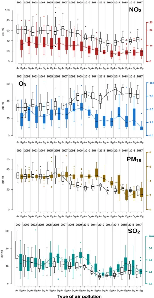
Fig. 3. Evolution of the average background (“Bg”, coloured box-whisker plots) and ambient (“Av”) pollutions, from 2001 to 2017, estimated for NO2, O3, PM10and SO2, at every monitoring site and for each year. Ambient pollution concentration is referred to the left axis and background pollution to the right one (inμg/m3).
error obtained in the testing fractions. In OK, the optimal variogram model was determined using the autofitVariogram function from the automap package (Hiemstra, Pebesma, Twenhofel, & Heuvelink, 2009) and later this result used as an input in the krige function (gstat package). Each of the pollution maps produced for each year has a 343.3 km2surface (16.8 km east-west x 20.5 km north-south) and are represented by 437 grid cells (23 cells × 19 cells), each of them cov-ering approximately an area of 0.8 km2. A general overview of the re-lationship of background levels of studied air pollutants and its tem-poral and spatial trends were later obtained by means of multivariate analysis (Principal Components Analysis -PCA-). PCA was performed using the dudi.pca function from ade4 package (Dray & Dufour, 2007) in R.
3. Results and discussion
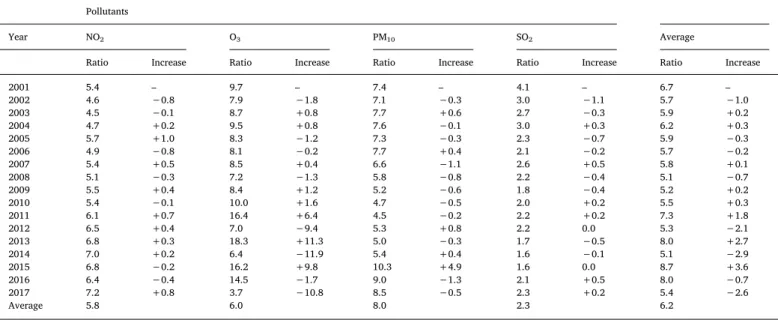
3.1. Evolution of the ambient and background pollution: 2001–2017 Fig. 3shows the evolution of average background pollution esti-mated at monitoring sites illustrated as coloured box-whisker plots, and compared to ambient pollution as a reference (white box-whisker plots). Trends are indicated with a joining line through the median of each box-whisker plot. As it can be seen in thisfigure, the quantitative difference between the background and ambient pollution differs ac-cording to the studied air pollutant. Remarkably, this difference re-mains practically constant for NO2and with few differences for PM10 and SO2. Regarding O3, this difference makes clearer from 2009 on-wards with a downward trend of the background pollution drawing a distinction with the ambient pollution. The quantitative relation be-tween the background and ambient air pollution (ratio) is numerically provided inTable 1. The increase and decrease of this ratio between the ambient and background pollution concentrations for NO2, PM10and SO2practically remains constant for the 17 years period. With regard NO2and PM10, this ratio estimates that background air pollution is on average about seven times lower (6.9 units) than ambient pollution and two times lower (2.3 units) for SO2. For O3, it can be distinguished two epochs (2001–2009 and 2010–2017) with the ratio increasing from 8.5 to 11.6, respectively. Considering all the air pollutants, this ratio is estimated in 6.2 units.
Except for O3, the studied background pollution trends mimic the one from the ambient pollution, suggesting that the prevalence of the former could be likewise affected by meteorological and physical
factors that influence the levels of ambient pollution in Madrid. The contributions from non-local (regional) sources to the estimated levels of background pollution is likely to be present, although their study would require a more detailed investigation. The abrupt decrease of background O3from 2009 to 2010 indicates that a lag of one year is exhibited with respect the beginning of the emission cut downs of O3 precursors due to economic recession (2008). The median location within the box-whisker plots for all the pollutants is irregularly placed across years, indicating the departure of the normal statistical dis-tribution of background concentrations on Madrid sites. In the PM10 case, from 2008 onwards the length of the box-whisker plot indicates that the PM10pollution is approximately similar for most of the mon-itoring sites studied.
Exploration of new threshold values of air pollutants below which no damage to health is observed have been set as a priority by World Health Organization (2016;WHO, 2003). To this regard, the presented levels of background pollution and its spatial analysis (provided in next section) are proposed as suitable concentrations levels for investigating their possible association with health outcomes detected in Madrid. Complementarily, one of the uses of these estimates can be also their inclusion as inputs or covariates in environmental epidemiological studies dealing with health outcomes.
3.2. Spatial analysis of background pollution
The choice of spatial unit analysis has important implications for results of epidemiological studies (Fecht et al., 2016). To better un-derstand the possible adverse health effects associated with exposure to background air pollution, maps given inFigs. 4 and 5for NO2and O3, respectively, provide sufficient detail to investigate such associations by Madrid's geographical zones. The same consideration is valid for PM10 and SO2maps (Figs. SM.2 and SM.3, respectively). The spatial dynamic of background pollution for all the studied pollutants is difficult to assess. Mainly, this is due to the urban heat island effect present in Madrid (Salamanca, Martilli, & Yagüe, 2012;Yagüe, Zurita, & Martínez, 1991) that affects not only the dynamics of pollutants beyond the me-teorological and physical factors, but also the regional contributions to the background pollution originated in adjacent municipalities from the Madrid metropolitan area. These contributions are strongly dominated by the road traffic sector (Borge et al., 2014). In these maps, two dis-tinct pollution nuclei can be differentiated, namely, the Madrid's urban core delimited by the M-30 ring road (inner position,Fig. 1) and the Table 1
Ratio between the average and background pollution annual mean values for all the studied sites in Madrid from 2001 to 2017. Pollutants
Year NO2 O3 PM10 SO2 Average
Ratio Increase Ratio Increase Ratio Increase Ratio Increase Ratio Increase
2001 5.4 – 9.7 – 7.4 – 4.1 – 6.7 – 2002 4.6 −0.8 7.9 −1.8 7.1 −0.3 3.0 −1.1 5.7 −1.0 2003 4.5 −0.1 8.7 +0.8 7.7 +0.6 2.7 −0.3 5.9 +0.2 2004 4.7 +0.2 9.5 +0.8 7.6 −0.1 3.0 +0.3 6.2 +0.3 2005 5.7 +1.0 8.3 −1.2 7.3 −0.3 2.3 −0.7 5.9 −0.3 2006 4.9 −0.8 8.1 −0.2 7.7 +0.4 2.1 −0.2 5.7 −0.2 2007 5.4 +0.5 8.5 +0.4 6.6 −1.1 2.6 +0.5 5.8 +0.1 2008 5.1 −0.3 7.2 −1.3 5.8 −0.8 2.2 −0.4 5.1 −0.7 2009 5.5 +0.4 8.4 +1.2 5.2 −0.6 1.8 −0.4 5.2 +0.2 2010 5.4 −0.1 10.0 +1.6 4.7 −0.5 2.0 +0.2 5.5 +0.3 2011 6.1 +0.7 16.4 +6.4 4.5 −0.2 2.2 +0.2 7.3 +1.8 2012 6.5 +0.4 7.0 −9.4 5.3 +0.8 2.2 0.0 5.3 −2.1 2013 6.8 +0.3 18.3 +11.3 5.0 −0.3 1.7 −0.5 8.0 +2.7 2014 7.0 +0.2 6.4 −11.9 5.4 +0.4 1.6 −0.1 5.1 −2.9 2015 6.8 −0.2 16.2 +9.8 10.3 +4.9 1.6 0.0 8.7 +3.6 2016 6.4 −0.4 14.5 −1.7 9.0 −1.3 2.1 +0.5 8.0 −0.7 2017 7.2 +0.8 3.7 −10.8 8.5 −0.5 2.3 +0.2 5.4 −2.6 Average 5.8 6.0 8.0 2.3 6.2
Adolfo Suarez Madrid-Barajas airport area (site 27,Fig. 1). The 24 and 58 sites (left side, Fig. 1) correspond to suburban monitoring sites, and in particular thefirst one, with the largest public park in Madrid (Casa de Campo). It is worth to note that the quantitative variations in
background pollution levels (range of concentration values) are lower than in the ambient pollution case (Fig. 3).
InFig. 4, two epochs in NO2maps can be clearly distinguished, from 2001 to 2008 and from 2009 to 2017 years. During thefirst period, Fig. 4. Estimation of spatial distribution of background NO2concentrations, from 2001 to 2017.
airport and urban core show highest levels of background pollution, in thefirst case due to heavily trafficked hot spots, and in the second one, probably due to the air traffic. From 2008 ahead, the background pollution shows a steady decrease that determine lowest concentrations
until 2017. From 2012 onwards, the evolution of the background pol-lution is irregular considering the narrow interval showed (lower than five or 10 μg/m3).
The background O3 spatial gradients behaviour is approximately Fig. 5. Estimation of spatial distribution of background O3concentrations, from 2001 to 2017.
consistent with higher levels of O3ambient pollution at city outskirts. This can be appreciated during most of the years except higher levels of background pollution at specific monitoring sites from the urban core (e.g., 2002 and 2005). However, the association between NO2and O3 background levels cannot be easily established, probably due to the low concentration levels of the background fraction of both pollutants.
PM10background concentrations may serve as a proxy for traffic pollution, as reflected in higher concentrations estimated at traffic hot-spot sites during 2007, and 2011 to 2014. However, low levels of PM10 are approximately constants during the studied period. Typical con-tributions in Madrid for PM10background pollution could also be ex-plained by dust outbreaks from Sahara desert.
SO2 background concentrations are influenced, primarily by the industrial sector (including thermoelectric stations) and secondarily by traffic. Higher concentrations were estimated in 2001, 2005, and 2009. However, the SO2concentrations have been decreasing due to the po-licies and strategic measures applied, such as the burying of the M-30 road and the changing trend of power generation.
3.3. Multivariate analysis using the obtained estimates
In this section, it is presented a general overview of the multivariate relationships among pollutants, at the different studied sites and dates. PCA was performed over a dataset containing the background con-centration estimates obtained in previous sections conveniently iden-tified in time and location along the whole period of study.
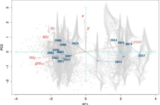
Fig. 6 illustrates the resulting factorial map, in which individual observations are projected (grey points) over the two first principal components resulting from PCA (PC1 and PC2), projection of numerical variables (red arrows) is overlapped, and projection of years (blue) is given as well. As usual in PCA, the angle between numerical variables projection's and principal components is related with the correlations between them and the length of projection with the importance in the first factorial axis. Also, projection of centroids with years allows to understand temporal trends. The PCA shows that NO2and PM10(in red) appear with a weak positive association (they project on the same di-rection with small angle between them), meaning that PM10tends to increase together with NO2, as well as O3tends to grow together with SO2. The georeference of each observation is represented in variables x and y, indicating the longitude and latitude where the measurements
were taken. As longitude (red arrow labeled with x) projects in the same direction of the second factorial axis (PC2), observations in I and II quadrants (upper part of thefigure) tend to be in the Eastern part of the city (longitude increases to the East), whereas III and IV quadrants are in the Western part. Thefigure indicates that the Eastern part of the city has typically higher O3and SO2concentrations. The former one accu-mulates in city outskirts as a consequence of traffic. The later comes mainly from power generation and is frequent in industrial areas, like those present in the metropolitan areas of big cities. In the Madrid's metropolitan area, NO2and PM10 levels, mainly produced by traffic congestions tend to be lower, as opposed to Madrid's city center where traffic congestion is intense and register higher values.
By projecting the years on top of this factorial map, it is seen that, in general, background air pollutant concentrations decrease along time (as years increase towards the right hand side of the map whereas the variables representing pollutants projects towards the left hand side of the map). It is also remarkable that between 2010 and 2011 there is a significant change in pollution. This is aligned with the requirement that European Commission sent to Spain on November 24, 2010 to activate measures to comply with the air quality standards from the Air Quality Directive 2008/50/CE, that caused the elaboration of the Spanish Royal Decree 102/2011, regarding improvements in quality of air.Fig. 6shows that the policies activated by 2011 effectively reduced the background pollution levels of the studied pollutants in Madrid. 3.4. Daily patterns of background pollution
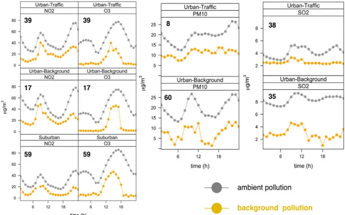
Existing studies have shown evidences of daily variation in exposure to ambient PM10, NO2, and O3, to be linked to acute pulmonary and cardiovascular outcomes. Moreover, levels considered generally safe by regulatory authorities have been suggested to also increase the daily and even hourly risk of adverse health outcomes (Lin et al., 2018). Delfino, Zeiger, Seltzer, Street, and McLaren (2002)predicted that the next phase of epidemiological research would use better spatially and temporally resolved data that take into account personal time-place-activity patterns and hourly exposures. For these reasons, the daily background pollution trend is briefly studied at selected monitoring sites in Madrid (Urban-traffic, urban-background and suburban) for all the considered pollutant.Fig. 7illustrates the evolution of background and average pollution at these sites. Remarkably, the daily evolution
Fig. 6. First factorial plane showing global relationships between pollutants, time and space (eigenvectors in red). (For interpretation of the references to colour in thisfigure legend, the reader is referred to the web version of this article.)
pattern of average and background pollution is similar for the studied air pollutants, even the typology of monitoring sites is different as well as the genesis and dynamic of the studied pollutants.
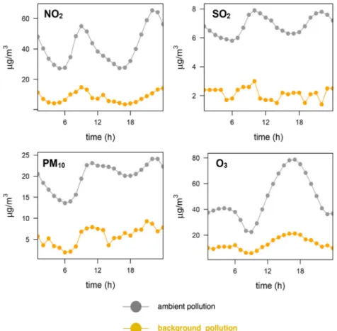
Fig. 8 shows the relation between the average and background pollution for 2017 considering all monitoring sites and air pollutants. These results show the similar dynamic experienced by the background levels with respect the ambient pollution, even the quantitative relation varies according to the hour of the day. The behaviour of this relation is less affected in the case of PM10, meanwhile in the case of O3 the change is evidenced from midday onwards, and from 18 h onwards in the case of NO2. Background values for SO2remain practically constant through the day.
3.5. Limitations and strengths
It is important to consider that during the studied period (2001 to 2017), the AQMN of Madrid has experienced relocation of monitoring sites and change the focus of the monitored pollutants, according to the new requirements from European legislation regarding the number of stations required in urban environments (Directive 2008/50/EC). This circumstance might prevent to obtain a consistent view of air quality evolution in the city. However, the spatiotemporal approach presented in this work is useful to impute all missing values in all locations along the period of study. The proposed methodology contributes to spatio-temporal modelling of exposure levels with robustness to possible re-location of monitoring stations. The single impact of rere-location is the uncertainty associated with the measurements, since the estimated one has higher variance, but allows integration of a whole geographical area in the analysis, regardless the continuity and length of the time series provided by every single monitoring station. It is important to clarify that, although the background pollution is influenced by local sources (Moreno et al., 2009), it can be less affected than ambient pollution when relocation schemes are performed. Secondly, the Ma-drid's relocation of sites was studied byMontero and Fernández-Avilés
(2018)with regard PM10ambient pollution. These authors concluded that the new pollution maps of the city obtained after relocating sites show a similar pattern that would have been provided by the previous configuration of sites.
Urban concentration levels depend on atmospheric phenomena that occur at different spatial scales, from transboundary scales to street levels of a few meters (Monteiro, Miranda, Borrego, & Vauard, 2007). Additionally, these levels present complex interactions with a large variety of chemical in the atmosphere, to not cite few the meteor-ological conditions affecting their dynamics. Up to now, no single model can describe the process consistently so a combination of models is needed to address such description (Borge et al., 2014). The model-ling results applied in this study could be integrated into other models in order to avoid failing to explain to what extent local and non-local sources contribute to the estimated background concentrations.
The background pollution and its spatial analysis can be helpful in environmental epidemiological studies concerning health effects de-tected in the studied area. Moreover, the estimation of the background pollution by this methodology could reduce the necessity of back-ground monitoring sites. To confirm the levels obtained by this odology only few of the existing sites would be necessary. This meth-odology would also provide important information to the population and can be applied to other forms of pollution as long as it is monitored at a convenient resolution. Air pollutions maps provide a complete air quality description, which can be helpful identifying new sources of emissions located inside of the monitored area.
4. Conclusions
In this study, the temporal and spatial scales of the background pollution were characterized during the period between 2001 and 2017, in Madrid (Spain). The difference between the ambient and background pollution between was practically constant for NO2 and with few significant differences for PM10and SO2. Regarding O3, this Fig. 7. Daily evolution of ambient and background pollution at different types (urban traffic, urban background and suburban) of monitoring sites, during 2017 (in μg·m−3). Bold numbers inside graphics identify monitoring sites.
difference makes clearer from 2009 onwards with a downward trend of the background pollution drawing a distinction with the ambient pol-lution. The ratio between the ambient and background concentration was constant for NO2, PM10 and SO2. For NO2and PM10, the back-ground pollution is on average six times lower and for SO2is around two times lower than the ambient pollution. Regarding O3, two epochs are distinguished (2001–2009 and 2010–2017), where the ratio in-creasing from 8.5 to 11.6, in each of them. The spatial analysis of background pollution is difficult to assess due to meteorological and physical factors and the regional contributions originated in adjacent municipals. Nevertheless, it can be distinguished two epochs regarding NO2 background concentrations (2001–2008 and 2009–2017). The high levels observed in thefirst period are strongly dominated by the heavily trafficked M-30 road and by air traffic. The O3spatial gradients are consistent and higher levels of ambient O3in outskirts. With regard to PM10, higher concentrations were estimated at traffic hot-sites in 2007, 2011 and 2014. Moreover, these events can be affected by dust outbreaks from Sahara desert. The SO2background pollution has been decreasing during the study period, but higher concentrations were estimated in 2001, 2005, and 2009. The background pollution esti-mates from the four studied air pollutants were used to build a spa-tiotemporal dataset to perform a global multivariate analysis. The PCA showed a significant decrease of background pollutant concentrations after the activation of measures to comply with the Air Quality Directive in Spain. Besides, global behaviours of pollutants in the Eastern city outskirt related to industry and traffic were also identified, showing the usefulness of getting these estimates for further analysis.
It has been seen that these models provide a comprehensive over-view, and probably a robust approach, of the complex estimation of background air pollution, which represents a chronic level of exposure to which the population is permanently exposed in cities. Complementarily, it is recommended their combination with other
modelling approaches, as new information inputs in epidemiological studies or to be extended to other forms of pollution. The performed modelling approaches are easy to implement and readily accessible at available R libraries or other commercial statistical software, making it possible to carry out all these analyses successfully without significant statistical expertise.
Disclaimer
The views expressed are purely those of the author and may not be regarded, in any circumstances, as stating an official position of the European Commission.
Appendix A. Supplementary data
Supplementary data to this article can be found online athttps:// doi.org/10.1016/j.compenvurbsys.2018.12.005.
References
Beelen, R., Hoek, G., Pebesma, E., Vienneau, D., de Hoogh, K., & Briggs, D. J. (2009). Mapping of background air pollution at afine spatial scale across the European Union. Science Total Environment, 635, 1852–1867.
Borge, R., Lumbreras, J., Pérez, J., de la Paz, D., Vedrenne, M., de Andrés, J. M., & Rodríguez, M. E. (2014). Emission inventories and modelling requirements for the development of air quality plans. Application to Madrid (Spain). Science Total Environment, 466-467, 809–819.
Borge, R., Artíñano, B., Yagüe, C., Gómez-Moreno, F. J., Siaz-Lopez, A., Sastre, M., ... Cristóbal, A. (2018). Application of a short term air quality action plan in Madrid (Spain) under a high-pollution episode - part I: Diagnostic and analysis from ob-servations. Science Total Environment, 635, 1561–1573.
Cheng, H., Kwong, J. C., Copes, R., Tu, K., Villeneuve, P. J., Donkelaar, A.v., ... Burnett, R. T. (2017). Living near major roads and the incidence of dementia, Parkinson's dis-ease, and multiple sclerosis: A population-based cohort study. The Lancet, 389, 718–726.
Fig. 8. Quantitative relation between ambient (grey colour) and background pollution (yellow colour) through the day considering all monitoring sites in Madrid and air pollutants. (For interpretation of the references to colour in thisfigure legend, the reader is referred to the web version of this article.)
Cuevas, C.A., Notario, A., Adame, J.A., Hilboll, A., Richter, A., Burrows, J.P., Saiz-López, A., 2014. Evolution of NO2 levels in Spain from 1996 to 2012. Nature Scientific Reports 4: 5887.
Delfino, R. J., Zeiger, R. S., Seltzer, J. M., Street, D. H., & McLaren, C. E. (2002). Association of asthma symptoms with peak particulate air pollution and effect modification by anti- inflammatory medication use. Environ. Health Perspectives, 110(10), A607.
Dray, S., & Dufour, A. B. (2007). The ade4 package: Implementing the duality diagram for ecologists. Journal of Statatistical Software, 22(4), 1–20.
Fecht, D., Hansell, A. L., Morley, D., Dajnak, D., Vienneau, D., Beevers, S., ... Gulliver, J. (2016). Spatial and temporal associations of road traffic noise and air pollution in London: Implications for epidemiological studies. Environmental International, 88, 235–242.
Gao, S., Yang, W., Zhang, H., Sun, Y., Mao, J., Ma, Z., ... Bai, Z. (2018). Estimating re-presentative background PM2.5 concentration in heavily polluted areas using base-line separation technique and chemical mass balance model. Atmosph. Environ. 174, 180–187.
Gómez-Losada, A., Pires, J. C. M., & Pino-Mejías, R. (2016). Characterization of back-ground air pollution exposure in urban environments using a metric base don Hidden Markov Models. Atmospheric Environment, 127, 255–261.
Gómez-Losada, A., Pires, J. C. M., & Pino-Mejías, R. (2018). Modelling background air pollution exposure in urban environments: Implications for epidemiological research. Environmental Modelling & Software, 106, 13–21.
Gräler, B., Pebesma, E., & Heuvelink, G. (2016). Spatio-Temporal Interpolation using gstat. The Royal Journal. 8(1), 204–218.
Hiemstra, P. H., Pebesma, E. J., Twenhofel, C. J. W., & Heuvelink, G. B. M. (2009). Real-time automatic interpolation of ambient gamma dose rates from the Dutch Radioactivity monitoring Network. Computational Geosciences, 35(8), 1711–1721. INE (2017). Instituto Nacional de Estadística.
Jerret, M., Arain, A., Kanaroglou, P., Beckerman, B., Potoglou, D., Sahsuvaroglu, T., ... Giovis, C. (2005). A review and evaluation of intraurban air pollution exposure models. Journal of Exposure Science & Environmental Epidemiology, 15, 185–204. Lao, X. Q., Zhang, Z., Lau, A. K. H., Chan, T. C., Chuang Chang, J., Lin, C., ... Chang, L.
(2018). Exposure to ambientfine particulate matter and semen quality in Taiwan. Occupational and Environmental Medicine, 75, 148–154.
Lee, B. L., Kim, B., & Lee, K. (2014). Air Pollution Exposure and Cardiovascular Disease. Toxicology Research, 30(2), 71–75.
Lepeule, J., Bind, M. A. C., Baccarelli, A. A., Koutrakis, P., Tarantini, L., et al. (2014). Epigenetic influences on associations between air pollutants and lung function in elderly men: The normative aging study. Environmental Health Perspectives, 122, 566–572.
Li, J., & Heap, A. D. (2011). A review of comparative studies of spatial interpolation methods in environmental sciences: Performance and impact factors. Ecological Information, 6, 228–241.
Li, J., & Heap, A. D. (2014). Spatial interpolation methods applied in the environmental sciences: A review. Environment Modulation Software, 53, 173–189.
Li, J., Heap, A. D., Potter, A., & Daniell, J. J. (2011). Application of machine learning methods to spatial interpolation of environmental. Environment Modulation Software, 26, 1647–1659.
Lin, H., Wang, X., Qian, Z. M., Guo, S., Yao, Z., Vaughn, M. G., ... Ma, W. (2018). Daily exceedance concentration hours: A novel indicator to measure acute cardiovascular effects of PM2.5 in six Chinese subtropical cities. Environmental International. 11, 117–123.
Madrid City Council.www.madrid.es[internet, retrieved 26th August, 2018]. MAPAM (Ministerio de Agricultura y Pesa, Alimentación y Medio Ambiente) (2017).
Evaluación de la calidad del aire en España, 2016. Madrid: MAPAM.
Menichini, E., Iacovella, N., Monfredini, F., & Turrio-Baldassarri, L. (2007). Atmospheric pollution by PAHs, PCDD/Fs and PCBs simultaneously collected at a regional back-ground site in Central Italy and at an urban site in Rome. Chemosphere, 69, 422–434. Monteiro, A., Miranda, A., Borrego, C., & Vauard, R. (2007). Air quality assessment for
Portugal. Science Total Environment, (1), 22–31.
Montero, J. M., & Fernández-Avilés, G. (2018). Functional kriging prediction of atmo-spheric particulate matter concentrations in Madrid, Spain: Is the new monitoring system masking potential public health problems? Journal of Cleaner Production, 175, 283–293.
Monzón, A., & Guerrero, M. J. (2004). Valuation of social and health effects of transport-related air pollution in Madrid (Spain). Science Total Environment, 334-335, 427–434. Moreno, T., Lavin, J., Querol, X., Alastuey, A., Viana, M., & Gibbons, W. (2009). Controls on hourly variations in urban background air pollutant concentrations. Atmospheric Environment, 43, 4178–4186.
R Core Team (2017). R: A language and environment for statistical computing. Vienna, Austria: R Foundation for Statistical Computing.
Saiz-López, A., Borge, R., Notario, A., Adame, J. A., de la Paz, D., Querol, X., ... Cuevas, C. A. (2017). Unexpected increase in the oxidation capacity of the urban atmosphere of Madrid, Spain. Nature Scientifics Reports, 7, 45956.
Salamanca, F., Martilli, A., & Yagüe, C. (2012). A numerical study of the urban Heat Island over Madrid during the DESIREX (2008) campaign with WRF and an evalua-tion of simple mitigaevalua-tion strategies. Internaevalua-tional Journal of Climatology, 32, 2372–2386.
Salvador, P., Artíñano, B., Alonso, D. G., Querol, X., & Alastuey, A. (2004). Identification and characterisation of sources of PM10 in Madrid (Spain) by statistical methods. Atmospheric Environment, 38(3), 435–447.
Salvador, P., Artíñano, B., Viana, M., Alastuey, A., & Querol, X. (2012). Evaluation of the changes in the Madrid metropolitan área infliencing air quality: Analysis of 1999-2008 temporal trend of particlaute matter. Atmospheric Environment, 57, 175–185. Tadic, J. M., Ilic, V., & Biraud, S. (2015). Examination of geostatistical and
machine-learning techniques as interpolators in anisotropic atmospheric environments. Atmospheric Environment. 111, 28–38.
Tonne, C., Basagaña, X., Chaix, B., Huynen, M., Hystad, P., Nawrot, T. S., ... Nieuwenhuijsen, M. (2017). New frontiers for environmental epidemiology in a changing world. Environment International, 104, 155–162.
Valverde, V., Pay, M. T., & Baldasano, J. M. (2016). Ozone attributed to Madrid and Barcelona on-road transport emissions: Characterization of plume dynamics over the Iberian Peninsula. Science Total Environment. 543, 670–682.
Visser, I., & Speekenbrink, M. (2010). depmixS4: an R package for hidden markov models. Journal of Statistic Software, 36(7), 1–21.
Weinmayer, G., Hennig, F., Fuks, K., Nonnemacher, M., Jakobs, H., Möhlenkamp, S., ... Heinz, N. (2015). Long-term exposure tofine particulate matter and incidence of type 2 diabetes mellitus in a cohort study: Effects of total and traffic-specific air pollution. Environmental Health, 14, 53.
Weisskopf, M., Seals, R., & Webster, T. F. (2018). Bias Amplification in Epidemiologic Analysis of Exposure to Mixtures. Environmental Health Perspectives, 126(4), 1–8. WHO (World Health Organization) (1980). Glossary on Air Pollution, WHO Regional
Publications, Eur. Series no. Copenhagen: Regional Office for Europe9.
WHO (World Health Organization) (2003). Health aspects of air pollution with particulate matters, ozone and nitrogene dioxide. Bonn, Germany: Report on WHO Working Group2003.
WHO (World Health Organization) (2016). Ambient air pollution: A global assessment of exposure and burden of disease. Geneva, Switzerland: WHO.
WHO (World Health Organization), 2006. Regional office for Europe. Air quality guide-lines. Global update (2005). Particulate matter, ozone, nitrogen dioxide and sulfur dioxide. Global update, 2005.
Wong, D. W., Yuan, L., & Perlin, S. A. (2004). Comparison of spatial interpolation methods for the estimation of air quality data. Journal of Exposure Science & Environmental Epidemiology, 14, 404–415.
Yagüe, C., Zurita, E., & Martínez, A. (1991). Statistical analysis of the Madrid urban heat island. Atmospheric Environment, 25B, 327–332.
Zucchini, W., & MacDonald, I. (2009). Hidden Markov Models for Time Series. An Introduction using R. New York: CRC Press.