Trends analysis of PM source contributions and chemical tracers in NE Spain during 2004–2014: a multi-exponential approach

(1)

www.atmos-chem-phys.net/16/11787/2016/ doi:10.5194/acp-16-11787-2016

Trends analysis of PM source contributions and chemical tracers in

NE Spain during 2004–2014: a multi-exponential approach

Marco Pandolfi1_{, Andrés Alastuey}1_{, Noemi Pérez}1_{, Cristina Reche}1_{, Iria Castro}1_{, Victor Shatalov}2_{, and} Xavier Querol1

1_{Institute of Environmental Assessment and Water Research, c/Jordi-Girona 18-26, 08034 Barcelona, Spain} 2_{Meteorological Synthesizing Centre, East, 2nd Roshchinsky proezd, 8/5, 115419 Moscow, Russia}

Correspondence to:Marco Pandolfi ([email protected])

Received: 14 January 2016 – Published in Atmos. Chem. Phys. Discuss.: 29 March 2016 Revised: 1 September 2016 – Accepted: 8 September 2016 – Published: 22 September 2016

Abstract.In this work for the first time data from two twin stations (Barcelona, urban background, and Montseny, re-gional background), located in the northeast (NE) of Spain, were used to study the trends of the concentrations of dif-ferent chemical species in PM10 and PM2.5along with the trends of the PM10 source contributions from the positive matrix factorization (PMF) model. Eleven years of chem-ical data (2004–2014) were used for this study. Trends of both species concentrations and source contributions were studied using the Mann–Kendall test for linear trends and a new approach based on multi-exponential fit of the data. Despite the fact that different PM fractions (PM2.5, PM10) showed linear decreasing trends at both stations, the contri-butions of specific sources of pollutants and of their chemi-cal tracers showed exponential decreasing trends. The differ-ent types of trends observed reflected the differdiffer-ent effective-ness and/or time of implementation of the measures taken to reduce the concentrations of atmospheric pollutants. More-over, the trends of the contributions of specific sources such as those related with industrial activities and with primary energy consumption mirrored the effect of the financial cri-sis in Spain from 2008. The sources that showed statistically significant downward trends at both Barcelona (BCN) and Montseny (MSY) during 2004–2014 were secondary sulfate, secondary nitrate, and V–Ni-bearing source. The contribu-tions from these sources decreased exponentially during the considered period, indicating that the observed reductions were not gradual and consistent over time. Conversely, the trends were less steep at the end of the period compared to the beginning, thus likely indicating the attainment of a lower limit. Moreover, statistically significant decreasing

trends were observed for the contributions to PM from the industrial/traffic source at MSY (mixed metallurgy and road traffic) and from the industrial (metallurgy mainly) source at BCN. These sources were clearly linked with anthropogenic activities, and the observed decreasing trends confirmed the effectiveness of pollution control measures implemented at European or regional/local levels. Conversely, at regional level, the contributions from sources mostly linked with natu-ral processes, such as aged marine and aged organics, did not show statistically significant trends. The trends observed for the PM10 source contributions reflected the trends observed for the chemical tracers of these pollutant sources well.

1 Introduction

(2)

Barm-padimos et al. (2012) have also shown that PM10 concen-trations decreased at a number of urban background (UB) and rural background stations in five European countries. Henschel et al. (2013) reported the dramatic decrease in SO2levels in six European cities, which reflected the reduc-tion in sulfur content in fuels, as part of European legisla-tion, coupled with the shift towards the use of cleaner fu-els. EEA (2013) also reported general decreases in NO2 con-centrations, even if they were lower compared to PM. How-ever, Henschel et al. (2015) showed that the NOx

concen-trations at traffic sites in many European cities remained un-changed, underlining the need of further regulative measures to meet the air quality standards for this pollutant. In fact an important proportion of the European population lives in ar-eas exceeding the AQ standards for the annual limit value of NO2, the daily limit value of PM10, and the health protec-tion objective of O3(EEA, 2013, 2015). PM10 and NO2are still exceeded mostly in urban areas, and especially at traf-fic sites (Harrison et al., 2008; Williams and Carslaw, 2011; EEA, 2013; among others). In Spain, for example, it has been reported that more than 90 % of the NO2 exceedances can be attributed to road traffic emissions (Querol et al., 2012). Guerreiro et al. (2014) furthermore evidenced the notable re-duction of ambient air concentration of SO2, CO, and Pb using data available in Airbase (EEA, 2013), covering 38 European countries. Querol et al. (2014) reported trends for 73 measurement sites across Spain including regional back-ground (RB), urban backback-ground (UB), traffic stations (TS), and industrial sites (IND). They observed marked downward trends for the concentrations of PM10, PM2.5, CO, and SO2 at most of the RB, UB, TR, and IND sites considered. Sim-ilarly, Salvador et al. (2012) detected statistically significant downward trends for the concentrations of SO2, NOx, CO

and PM2.5at most of the urban and urban-background mon-itoring sites in the Madrid metropolitan area during 1999– 2008. Cusack et al. (2012) and Querol et al. (2014) have also shown the statistically significant decreasing trends for many trace elements (Pb, Cu, Zn, Mn, Cd, As, Sn, V, Ni, Cr) at regional level in the northeast (NE) of Spain since 2002.

The observed reduction of air pollutants across Europe is the result of efficient emission abatement strategies, as for example those implemented in the Industrial Emission Di-rective (IPPC – Integrated Pollution Prevention and Control – and subsequent Industrial Emission Directive 1996/61/EC and 2008/1/EC), the Large Combustion Plant Directive (LCPD; 2001/80/EC), the EURO standards on road traffic emission (1998/69/EC, 2002/80/EC, 2007/715/EC), and the IMO (International Maritime Organization) directive on sul-fur content in fuel and SOx and NOx emissions from ships

(IMO, 2011; Directive 2005/33/EC). Additionally, the finan-cial crisis, causing mainly a reduction of the primary energy consumption from 2008 to 2009, contributed to the decrease of the ambient concentration of pollutants observed in Spain (Querol et al., 2014).

Moreover, national and regional measures for AQ have been taken in many European countries. In Spain a national AQ plan was approved in 2011 and updated in 2013 by the Council of Ministers of the government of Spain. Further-more, 45 regional and 3 local (city-scale) AQ plans have been implemented since 2004 in Spain. These AQ plans have mostly focused on improving AQ at major city centers and specific industrial areas.

Thanks to the aforementioned measures there is clear evi-dence that the concentrations of PM in many European coun-tries have markedly decreased during the last decades. How-ever, in spite of the above policy efforts, a significant propor-tion of the urban populapropor-tion in Europe lives in areas exceed-ing the World Health Organization (WHO) AQ standards, for example for PM2.5, PM10, and O3(EEA, 2013, 2015).

The analysis of the trends of the concentration of air pol-lutants helps in evaluating the effectiveness of specific AQ measures depending on the pollutant considered. Examin-ing data over time also makes it possible to predict future frequencies and/or rates of occurrence making future pro-jections. For the abovementioned reasons, the feasibility of studying the trends of the contributions to PM mass from specific pollutant sources, along with the trends of the chem-ical tracers of these sources, is especially attractive.

To the best of our knowledge, in the majority of stud-ies dealing with trend analysis, linear fits were applied by using Mann–Kendall (MK) or Theil–Sen methods (Theil, 1950; Sen, 1968), the latter being available, for example, in the Openair software (Carslaw, 2012; Carslaw and Ropkins, 2012). However, a linear fit of data does not always prop-erly represent the observed trends. As we will show, differ-ent abatemdiffer-ent strategies and periods of implemdiffer-entation may change from one pollutant to another, thus leading to dif-ferent trends for difdif-ferent pollutants, even over the same pe-riod. Thus, a nonlinear fit of the data may be strongly recom-mended at times.

(3)

Mediter-works

BCN measuring site before 2009 BCN measuring

site from 2009

Diagonal Av.

Unpaved parking

Barcelona Metrop. Area (BMA)

BMA

MSY measuring site

BCN MSY

SPAIN

BCN

MSY

Figure 1.Location of the Barcelona (BCN) and Montseny (MSY) measuring stations. Red full circle highlights the location of the BCN measuring station before 2009. Green full circle highlights the new location of the BCN (from 2009) and MSY measuring stations.

ranean, and, (b) in the use of a novel nonlinear approach for trend studies.

2 Measurement sites and methodology 2.1 Measurement sites

The Montseny measurement station (MSY, 41◦

46′

45.63′′

N, 02◦

21′

28.92′′

E; 720 m a.s.l.) is a regional background site in the NE of Spain, located in a regional natural park about 50 km to the NNE of the city of Barcelona (BCN) and 25 km from the Mediterranean coast (Fig. 1). This site is represen-tative of the typical regional background conditions of the western Mediterranean Basin (WMB), characterized by se-vere pollution episodes affecting not only the coastal sites closest to the emission sources, but also the more elevated ru-ral and remote areas inland (i.e., Pérez et al., 2008; Pey et al., 2010; Pandolfi et al., 2011, 2014). This station is part of the ACTRIS (www.actris.net) and GAW (www.wmo.int/gaw) networks, of the EMEP Program (http://www.emep.int/) and of the measuring network of the government of Catalonia.

The Barcelona measurement station (BCN, 41◦

23′

24.01′′

N, 02◦

06′

58.06′′

E; 68 m a.s.l.) is an

ur-ban background measurement site influenced by vehicular emissions from one of the main avenues of the city (Di-agonal Avenue) located at a distance of around 300 m (cf. Fig. 1). The BCN measurement site is part of the air quality measuring network of the government of Catalonia. The metropolitan area of Barcelona (BMA), with nearly 4.5 million inhabitants, covers a strip 8 km wide between the Mediterranean Sea and the coastal mountain range. Several industrial zones, power plants, and highways are located in the area, making this region one of the most polluted in the WMB (i.e., Querol et al., 2008; Amato et al., 2009; Pandolfi et al., 2012, 2013, 2014). At BCN the location of the measuring station changed in 2009 when it was moved by around 500 m (cf. Fig. 1). The effect of this change on PM measurements performed at BCN will be discussed later.

2.2 Real-time and gravimetric PM measurements

(4)

were corrected by comparison with 24 h gravimetric mass measurements of PMx(Alastuey et al., 2011).

For gravimetric measurements, 24 h PMx samples were collected at both stations every 3–4 days on 150 mm quartz micro-fiber filters (Pallflex QAT and Whatman) with high-volume samplers (DIGITEL DH80 and/or MCV CAV-A/MSb at 30 m3h−1_{). The mass of PM}

10and PM2.5samples collected on filters was determined using the EN 12341 and the EN14907 gravimetric procedures, respectively.

2.2.1 PM chemical speciated data

Once the gravimetric mass was determined from filters, the samples were analyzed with different techniques, includ-ing acidic digestion (1/2 of each filter; HNO3: HF : HClO4), water extraction of soluble anions (1/2 of each filter), and thermal-optical analysis (1.5 cm2_{sections). Inductively} cou-pled atomic emission spectrometry, ICP-AES, (IRIS Advan-tage TJA Solutions, THERMO) was used for the determi-nation of the major elements (Al, Ca, Fe, K, Na, Mg, S, Ti, P), and inductively coupled plasma mass spectrometry, ICP-MS, (X Series II, THERMO) for the trace elements (Li, Ti, V, Cr, Mn, Co, Ni, Cu, Zn, As, Se, Rb, Sr, Cd, Sn, Sb, Ba, rare earths, Pb, Bi, Th, U). Ionic chromatography was used for the concentrations of NO−₃, SO2₄−, and Cl−

, whereas NH+₄ was determined using a specific electrode MODEL 710 A+, THERMO Orion. The levels of organic carbon (OC) and elemental carbon (EC) were determined using a thermal-optical carbon analyzer (SUNSET), using protocol EUSAAR_2 (Cavalli et al., 2010). Other analytical details may be found in Querol et al. (2008).

Following the above procedures, a total of 1093 PM10and 794 PM2.5filters were collected and analyzed at MSY dur-ing the period 2004–2014. At BCN the collected filters were 1037 and 1063 in PM10and PM2.5, respectively.

2.3 Positive matrix factorization (PMF) model

The PMF model (PMFv5.0, EPA) was applied to the col-lected daily PM10speciated data for source identification and apportionment at both sites. Detailed information about the PMF model can be found in literature (Paatero and Tapper, 1994; Paatero, 1997; Paatero and Hopke, 2003; Paatero et al., 2005). The PMF model is a factor analytical tool, reduc-ing the dimension of the input matrix to a limited number of factors (or sources), and it is based on the weighted least-squares method. Thus, most important in PMF applications is the estimation of uncertainties of the chemical species in-cluded in the input matrix. In the present study, individual uncertainties and detection limits were calculated as in Es-crig et al. (2009) and Amato et al. (2009). Thus, both the an-alytical uncertainties and the standard deviations of species concentrations in the blank filters were considered in the un-certainties calculations. The signal-to-noise ratio (S/N) was estimated starting from the calculated uncertainties and used

as a criterion (S/N> 2) for selecting the species used within the PMF model. In order to avoid any bias in the PMF re-sults, the data matrix was uncensored (Paatero, 2004). The PMF was run in robust mode (Paatero, 1997), and rotational ambiguity was handled by means of the FPEAK parameter (Paatero et al., 2005). The optimal number of sources was selected by inspecting the variation of the objective function

Q(defined as the ratio between residuals and errors in each data value) with a varying number of sources (i.e., Paatero et al., 2002) and by studying the physical meaningfulness of the calculated factors.

2.4 Mann–Kendall (MK) fit

The purpose of the Mann–Kendall (MK) test (Mann, 1945; Kendall, 1975; Gilbert, 1987) is to statistically assess whether there is a monotonic upward or downward trend of the variable of interest with time. A monotonic upward (downward) trend means that the variable consistently in-creases (dein-creases) through time. The Mann–Kendall test tests the null hypothesis H0 of no trend, i.e., the observa-tions are randomly ordered in time, against the alternative hypothesis,H1, where there is an increasing or decreasing monotonic trend. The main advantage of the Mann–Kendall test is that data need not conform to any particular distribu-tion and missing data are allowed. To estimate the slope of the trend, Sen’s method was used (Salmi et al., 2002). 2.5 Multi-exponential (ME) fit

(5)

In-tegrated Assessment Modelling (CIAM; http://www.iiasa.ac. at/~rains/ciam.html). In 2014 the TFMM initiated an exercise dedicated to assessing the efficiency of CLRTAP air pollution mitigation strategies over the past 20 years, evaluating the benefit of its main policy instruments. Within this exercise a piece of software was made available by EMEP/MSC-E, with the aim of studying nonlinear trends. Annual, monthly, and daily resolution data can be analyzed with the help of this program. Since in this paper we will apply the program to annual averages of species concentrations and source con-tributions, we restrict the description of the multi-exponential approximations to this case. In particular, seasonal variations are not taken into consideration. The basic equations solved by the program for this particular case (annual averages) are reported below:

Ct=a1·exp

−t τ1

+a2·exp

−t τ2

+

. . .+an·exp

−t τn

+ωt, (1)

whereCt are the values of the considered time series, with t=1,. . ., N, N being the length of the series (years),τn are

the characteristic times of the considered exponential,anare

constants, andωt are the residue values. In the case of

sin-gle exponential decay (n=1) the characteristic timeτ is the time at which the pollutant concentration is reduced to 1/e (i.e., 0.3678) times its initial value. The main difference be-tween linear and exponential fit is that in the latter case, the trend is not gradual and constant over time. For an exponen-tial trend the absolute (µg m−3_{) reduction per year decreases} with time, being the highest at the beginning of the period. Conversely, for a linear fit, the absolute reduction is constant over time. For an exponential fit, the lower the characteris-tic timeτ, the more rapidly the considered quantity vanishes. Deviations from single exponential fit can be taken into ac-count introducing more exponential terms. In this work, for example, two exponential terms were sometimes used. In this case two characteristic times are calculated by the software. If the decrease of the considered quantity is very sharp at the beginning of the period (more than single exponential), then bothτ1andτ2are positive. Conversely, one exponential term with negativeτ takes possible increase of the quantity at the end of the period into account. Bothτnandanare calculated

by the program by means of the least-squares method, mini-mizing the residueω, and the statistically significance of the exponential fit is provided by means of thepvalue. The num-ber of exponential terms that should be included into the ap-proximation can be evaluated using F-statistics (i.e., Smith, 2002). For example, the F-statistics for the evaluation of the statistical significance of the second term in equation (1) for

n=2 can be calculated as

F = (SS1−SS2)

2·s , (2)

where SS1and SS2are sums of squares of residual compo-nent for approximations with one and two expocompo-nential terms, respectively, and s is the estimate of standard deviation of residual component. This statistic approximately follows the Fisher distribution, with 2 and N−2◦

of freedom. The sec-ond exponential is considered to be significant ifF exceeds the corresponding threshold value at the chosen significance level.

The following parameters can be calculated from Eq. (1):

total reduction: TR= Cbeg

−Cend Cbeg

=1−Cend

Cbeg

(3) annual reduction for yeari: Ri =

1Ci Ci

=1−Ci+1 Ci

(4)

average annual reduction:Rav=1−

Cend Cbeg

_N1₋₁

, (5)

whereCbegandCendare the first and the last points, respec-tively, of the exponential fit. The formula for the calculation of the average annual reduction takes into account that the ra-tioCi+1/Ci is a multiplicative quantity, so that geometrical

mean of ratios should be used. The relative contribution of residues (residual component: RC) is calculated as the stan-dard deviation of the ratios between the residue values of the fitωt(cf. Eq. 1) and the main component of the fit.

The MSC-E also proposed a statistic that measures the de-viation of the obtained trend from the linear one (nonlinear-ity parameter: NL). A trend is defined as linear if the NL parameter is lower than 10 %, indicating a small difference between ME and MK fits (Shatalov et al., 2015). In the fol-lowing, the reported trends were analyzed using the MK test for NL < 10 % and the ME test for NL > 10 %. A more de-tailed description of the multi-exponential approach is avail-able in the TFMM wiki and in the MSC-E technical report 2015 (Shatalov et al., 2015).

3 Results

Results are presented and discussed in the following order. In Sect. 3.1, we compare the trends at both stations of PMx

(6)

Table 1.Trends of different PM mass fractions from gravimetry (grav) and optical (OPC) measurements at BCN (italic) and MSY (2004-2014). TR (%) is the total reduction; RC (%) is the residual component. Significance of the trends following the Mann–Kendall test: ∗∗∗₍_p_{value < 0.001),}∗∗₍_p_{value < 0.01),}∗₍_p_{value < 0.05),}₊₍_p_{value < 0.1).}

PMx PMx Mann–Kendall fit

Fraction Conc. 2004 Conc. 2014 pvalue Trend TR RC

(µgm−3) (µgm−3) (µgm−3yr−1) ( %) ( %)

PM10(grav.) 41.1 19.2 ∗∗∗ −2.83 59.2 8.5

19.2 13.9 −0.17 10.5 17.6

PM2.5(grav.) 31.6 13.2 ∗∗∗ −2.03 60.1 7.9

16.2 9.8 + −0.33 25.6 17.3

PM10(OPC) 39.1 19.8 ∗∗∗ −2.20 50.4 10.0

18.6 12.3 −0.13 7.8 16.9

PM2.5(OPC) 27.1 12.9 ∗∗ −1.55 49.6 9.8

16.5 9.3 + −0.26 21.2 17.5

to 13 years). The gravimetric concentrations of PM2.5 mea-sured at MSY were used with this aim. Then, in Sect. 3.3, we present and discuss the trends at both stations of chemi-cal species from filters in both PM10and PM2.5. In Sect. 4.0 we discuss the sources of pollutants identified by the PMF model in PM10at both sites. Finally, we present and discuss the trends of PM10 source contributions at BCN and MSY (Sect. 4.1), providing possible explanations for the observed trends. Conclusions are reported in Sect. 5.

3.1 Trends of PM: comparison between gravimetric and real-time optical measurements

Annual data coverage is an important factor to take into ac-count in order to study trends of a given parameter. The gravimetric PM measurements, from which chemical speci-ated data are obtained, are typically performed with rather low frequency over 1 year. In our case, the annual data cov-erage of gravimetric measurements was around 20–30 % at both Barcelona and Montseny. In this section, we compare the trends of PM concentrations from gravimetric and real-time optical measurements (Table 1). Given that the trends of the considered PMx fractions were linear at both sites

(NL < 10 %), only results from MK test were reported in Ta-ble 1. However, we will show later (Sect. 4.1) that the contri-butions from specific PM10 pollutant sources, mainly those related with anthropogenic activities, showed nonlinear (i.e., exponential) decreasing trends, thus mirroring the different effectiveness of the mitigation strategies depending on the source of pollutants considered.

As reported in Table 1, statistically significant decreas-ing trends were observed for the considered PM size fractions at BCN (−2.20 µg m−3_yr−1 _with _p_{< 0.001 for} PM10 and −1.55 µg m−3yr−1 with p< 0.01 for PM2.5 from OPC measurements), whereas at Montseny, only the PM2.5fraction showed a slightly significant decreasing trend (−_{0.26 µg m}−3_yr−1_;p< 0.1 from OPC measurements). To-tal reduction (TR) ranged between 50.4 % (OPC PM10 at

BCN) and 7.8 % (OPC PM10 at MSY), and the residual component (RC) was lower than 18 %, reflecting the good-ness of the linear (MK) fit used. It must be noted that the higher p-values, magnitude of the trends, and TR observed at BCN compared to MSY was likely due to the change of the measuring station in 2009 in BCN (cf. Fig. 1). Based on the comparison between simultaneous PMx chemical

spe-ciated data collected at both BCN measurement sites dur-ing 1 month (not shown), we concluded that after 2009, the BCN measuring site was less affected by mineral matter and, to a lesser extent, by road traffic emissions, both being im-portant sources of PM in Barcelona. In Fig. 1 we highlight the proximity of the BCN measuring station before 2009 to an unpaved parking area and different construction works. The effect of the change of the station in BCN in 2009 on PM10 gravimetric measurements is reported in the Supple-ment (Fig. S1). However, despite the change of the station, the comparison between BCN and MSY for specific chem-ical species and pollutant sources not linked with mineral matter and road traffic emissions was possible.

(7)

Table 2.Mann–Kendall and multi-exponential trends of different chemical species in PM10at BCN (italic) and MSY. Type of trend: linear

(L), single exponential (SE), double exponential (DE);a(µgm−3)andτ(yr) are the constants and the characteristic times, respectively, of the exponential data fittings; NL (%) is the nonlinearity; TR (%) is the total reduction; RC (%) is the residual component; ns denotes not statistically significant; ni denotes not included. Significance of the trends:∗∗∗(pvalue < 0.001),∗∗(pvalue < 0.01),∗(pvalue < 0.05),+

(pvalue < 0.1).

PM₁₀(BCN; MSY) Mann– Multi-exponential fit Kendall fit

Specie Concentration Concentration Fit NL pvalue Trend a τ Trend TR RC 2004 (µgm−3₎ _{2014 (µgm}−3₎ _type _{( %)} _(µgm−3_yr−1₎ _(µgm−3₎ _(yr) _(µgm−3_yr−1₎ _{( %)} _{( %)}

Pb 0.02685 0.00694 SE 27 ∗∗∗ _0.03246 _6.12 ₋_0.00222 ₈₀ ₁₇

0.00481 0.00190 SE 11 ** 0.00553 10.22 −0.00031 62 13

Cd 0.00043 0.00015 SE 19 ∗∗∗ _0.00048 _7.59 ₋_3.10E-5 ₇₃ ₁₇

0.00017 0.00006 SE 18 ∗∗ _0.00018 _7.92

−1.12E-5 72 16

As 0.00094 0.00036 SE 14 ∗∗∗ _0.00118 _9.11 ₋_7.07E-5 ₆₇ ₁₁

0.00029 0.00017 L < 10 ∗∗∗

−1.29E-5 50 9

V 0.01116 0.00454 SE 12 ∗∗ _0.01502 _10.04 ₋_0.00086 ₆₃ ₁₇

0.00328 0.00175 L < 10 ∗∗

−0.00022 59 15

Ni 0.00531 0.00284 SE 11 ∗∗∗ _0.00678 _10.61 ₋_0.00037 ₆₁ ₁₆

0.00155 0.00100 L < 10 ∗∗ ₋_7.10E-5 ₄₃ ₂₀

Sn ni ni

0.00127 0.00057 L < 10 ∗ ₋_3.65E-5 ₃₉ ₁₆

Cu ni ni

0.00420 0.00216 L < 10 ∗ ₋_0.00014 ₃₆ ₂₀

Sb ni ni

0.00058 0.00025 SE 11 ∗∗ _0.00064 _10.46 ₋_3.57E-5 ₆₂ ₁₃ SO2−

4 5.74436 2.28596 SE 12

∗∗∗ _6.56033 _9.81

−0.37868 64 12

2.84849 1.67712 L < 10 ∗∗ ₋_0.11836 ₄₂ ₁₈ NO−

3 5.07816 1.72401 SE 12

∗∗ _6.49890 _9.83

−0.37484 64 15

1.80724 0.67419 L < 10 ∗∗

−0.10593 54 13

NH+₄ 1.92062 0.57008 SE 12 ∗∗∗ 1.90645 9.64 −0.11095 65 14

1.14268 0.40135 SE 13 ∗ _1.28868 _9.26

−0.07640 66 22 Al₂O₃ ni ni

0.72357 0.46382 L < 10 ∗

−0.02383 34 18

Ca ni ni

0.42703 0.28279 L < 10 ∗ ₋_0.01638 ₃₈ ₁₇

Fe ni ni

0.22371 0.14895 L < 10 + −0.00593 6 44

Na 1.02188 0.77408 L <10 ∗ −0.03943 34 12

ns

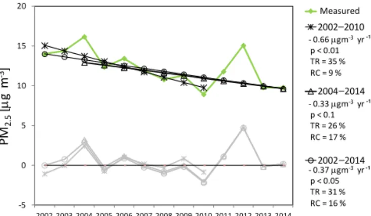
3.2 Trends of PM: comparison among different periods

In this study we used the period 2004–2014 for trends anal-ysis, given that gravimetric PM2.5 measurements at BCN have been available since 2004. Conversely, at MSY PM2.5, gravimetric measurements started in 2002. Figure 2 shows the trends of PM2.5 concentrations at MSY, calculated us-ing the MK test for the three different periods. The ME test was not used here given that the observed trends were lin-ear (NL < 10 %). The period 2002–2010 was the period con-sidered in the paper from Cusack et al. (2012) presenting the trends of PM2.5 gravimetric mass and chemical species at MSY. The period 2002–2014 is the largest period, with PM2.5 filter measurements available at the time of writing. The trend observed at MSY for the PM2.5 fraction during 2004–2014 confirmed what was already observed by Cusack

(8)

-5 0 5 10 15 20

2002 2003 2004 2005 2006 2007 2008 2009 2010 2011 2012 2013 2014

2010 2014 2014

2002 2003 2004 2005 2006 2007 2008 2009 2010 2011 2012 2013 2014

2002 2010 2014 2014 2004 2014 2002-2014 2002 2014

- 0.66 mgm-3_yr

p < 0.01 TR = 35 % RC = 9 %

- 0.33 mgm-3_yr

p < 0.1 TR = 26 % RC = 17 %

- 0.37 mgm-3_yr

p < 0.05 TR = 31 % RC = 16 %

PM 2 .5 [ m g m ] 3--1 -1 -1 – – – Measured

Figure 2. Mann–Kendall fit of PM2.5 trends at MSY station

for the periods 2002–2010 (as in Cusack et al., 2012), 2004– 2014 (this work), and 2002–2014 (largest period available in the

time of writing). The magnitude of the trends (µgm−3_yr−1_),

p value, total reduction (TR), and residual component (RC) are

reported. Significance of the trends following the Mann–Kendall test:∗∗∗₍_p_{value < 0.001),}∗∗₍_p_{value < 0.01),}∗₍_p_{value < 0.05),}

+(pvalue < 0.1).

mass concentration in 2012 (cf. Fig. 2). Chemical PM2.5 spe-ciated data revealed that this increase was partly driven by organic matter showing a mean annual concentration in 2012 higher by around 20 % compared to the 2004–2014 average. 3.3 Trends of chemical species

The trends of the annual mean concentrations of chemical species at BCN and MSY are reported in Table 2 (for PM10) and Table 3 (for PM2.5). Figure 3 (for BCN) and Fig. 4 (for MSY) show the trends of chemical species in PM10. In Ta-bles 2 and 3 and Figs. 3 and 4, only the species that have statistically significant trends were reported.

As already noted we assume that the change of the station in BCN in 2009 affected the trends of the concentrations of OC, EC, Cu, Sn, Sb, and Zn (mainly traffic tracers), Al2O3, Ca, Mg, Ti, Rb, Sr (crustal elements related with both nat-ural and anthropogenic sources), and Fe (traffic and crustal tracer). These chemical species at BCN were removed from Tables 2 and 3 and from Fig. 3.

Other species measured in BCN were not affected by the change of the station. These are SO2₄−, NH+₄, V, Ni (related with heavy oil combustion in the study area according to source apportionment results, cf. Par. 4), Pb, Cd, and As (re-lated with industrial/metallurgy activities), Na and Cl (sea spray), and NO−₃. Although nitrate particles in Barcelona were mainly from traffic, the concentrations of these particles were not strongly affected by the change of the station due to their secondary origin. The MSY station will be considered as reference station given that no location change occurred at this monitoring site during the study period.

Statistically significant exponential trends (p< 0.01 or 0.001) were mainly observed for the industrial tracers (Pb,

Cd, As) in both PM10and PM2.5. For these elements TR was high and around 50–80 % in PM10 and 67–81 % in PM2.5. The RCs were lower than 20 %, thus suggesting the good-ness of the exponential fits used to study the trends of these species. Exponential fits were needed on average, indicat-ing that the trends were not gradual and consistent over time and that the effectiveness of the control measures for these pollutants was stronger at the beginning of the pe-riod under study (2004–2009 approximately) compared to the end of the period (Figs. 3 and 4). This is also evident by comparing the linear MK fit (dashed black line) with the ME fit (red line) in Figs. 3 and 4. In PM10 the magni-tudes of the trends ranged from−_{0.00222 (Pb;}p< 0.001) to −_3.10×₁₀−5_{µg m}−3_yr−1_(Cd;p< 0.001) at BCN and from −0.00031 (Pb;p< 0.01) to−1.12×10−5_{µg m}−3_yr−1_(Cd; p< 0.01) at MSY. In PM2.5the magnitudes of the trends were similar and ranged between−0.00163 µg m−3_yr−1_(Pb;_p_< 0.001) and −3.11×10−5_{µg m}−3_yr−1 _(Cd; _p_{< 0.001) at} BCN and between −0.00049 µg m−3_yr−1 _(Pb; _p_{< 0.001)} and −1.35×10−5_{µg m}−3_yr−1 _(Cd; _p_{< 0.001) at MSY.} Similar magnitude of the trends for these species in both PM fractions at both sites confirmed the common origin of these elements and the impact at regional scale of industrial sources. For Pb and Cd, the characteristic time (τ )of the ex-ponential trends was similar at both sites, whereas for As it was higher due to the slightly less intense exponential down-ward trend observed for As compared to Cd and Pb. Note that the PMF analysis (cf. Sect. 4) revealed that the concen-trations of As were explained by multiple sources (especially at BCN), whereas the industrial/metallurgy source alone ex-plained more than around 70 % of Pb and Cd concentrations (not shown). The implementation of the IPPC Directive in 2008 in Spain is the most probable cause for this downward trend. The decrease observed for Pb, Cd, and As may also be attributed to a decrease in the emissions from industrial production (smelters; Querol et al., 2007) at a regional scale around Barcelona.

The concentrations of V and Ni in Barcelona in both PM10 and PM2.5 fractions showed very similar exponential decreasing trends. Similar characteristic times (around 10– 11 years), TR (around 59–63 %), and RC (15–17 %) in both fractions suggested the common and mainly fine origin of these two elements. At MSY, V and Ni showed linear trends likely because of the higher distance of the MSY station to the sources of V and Ni (shipping and, before 2008, energy production) compared to BCN. Note also that the NL pa-rameter for BCN V and Ni was around 10–12 %, indicating that in this case the exponential fit did not differ very much from the linear one. Total reduction for V and Ni at MSY was around 59–64 and 42–43 %, respectively, and RCs were lower than 24 %.

(9)

ob-Table 3.Mann–Kendall and multi-exponential trends of different chemical species in PM2.5at BCN (italic) and MSY. Type of trend: linear

(L), single exponential (SE), double exponential (DE);a(µgm−3)andτ(yr) are the constants and the characteristic times, respectively, of the exponential data fittings; NL (%) is the nonlinearity; TR (%) is the total reduction; RC (%) is the residual component; ns denotes not statistically significant; ni denotes not included. Significance of the trends:∗∗∗(pvalue < 0.001),∗∗(pvalue < 0.01),∗(pvalue < 0.05),+

(pvalue < 0.1).

PM₂.5(BCN;MSY) Mann–Kendall fit Multi-exponential fit

Specie Concentration Concentration Fit NL pvalue Trend a τ Trend TR RC 2004 (µgm−3₎ _{2014 (µgm}−3₎ _type _{( %)} _(µgm−3_yr−1₎ _(µgm−3₎ _(yr) _(µgm−3_yr−1₎ _(%) _(%)

Pb 0.02117 0.00500 SE 27 ∗∗∗ _0.02390 _6.24 ₋_0.00163 ₈₀ ₁₃

0.00642 0.00149 SE 28 ∗∗∗ _0.00716 _6.08 ₋_0.00049 ₈₁ ₁₈

Cd 0.00041 0.00011 SE 23 ∗∗∗ _0.00047 _6.81

−3.11E-5 77 13

0.00020 0.00005 SE 23 ∗∗∗ _0.00020 _6.77 ₋_1.35E-5 ₇₇ ₁₈

As 0.00069 0.00027 SE 14 ∗∗∗ _0.00091 _9.00 ₋_5.43E-5 ₆₇ ₁₁

0.00029 0.00013 SE 15 ** 0.00033 8.56 −2.04E-5 69 19

V 0.00823 0.00368 SE 11 ∗∗ 0.01121 11.13 −0.00061 59 16

0.00271 0.00130 L < 10 ∗∗ ₋_0.00017 ₆₄ ₂₄

Ni 0.00402 0.00185 SE 10 ∗∗ _0.00498 _11.23 ₋_0.00027 ₅₉ ₁₅

0.00189 0.00080 SE 13 ∗∗ _0.00205 _9.36

−0.00012 42 21

Sn ni ni

0.00157 0.00043 L < 10 ∗∗∗ ₋_0.00084 ₆₁ ₁₂

Cu ni ni

0.00394 0.00113 SE 14 ∗∗ 0.00426 8.99 −0.00026 67 13

Sb ni ni

0.00053 0.00015 DE 48 ∗∗ _0.00069 _4.52 ₋_3.86E-5 ₇₀ ₁₆ 1.3E-6 −2.50

SO2₄− 4.86564 1.92388 SE 12 ∗∗∗ _5.64582 _9.69 ₋_0.32778 ₆₄ ₉

2.98922 1.43381 L < 10 ∗∗

−0.16222 54 15

NO−

3 3.45513 0.86002 SE 19

∗∗∗ _4.14459 _7.61

−0.26753 73 16

1.66095 0.29452 SE 30 ∗∗∗ _1.96014 _5.81 ₋_0.13550 ₈₂ ₂₁ NH+

4 2.19735 0.68393 SE 11

∗∗∗ _2.27813 _10.53

−0.12701 61 15

1.39366 0.48049 SE 18 ** 1.62588 7.94 −0.10266 72 14 Al₂O₃ ni ni

0.30245 0.10153 SE 13 ∗ _0.26678 _9.36

−0.01574 66 35

Ca ni ni

0.11478 0.06540 L < 10 + −0.00494 50 33

Fe ni ni

0.09679 0.03716 L < 10 ∗ ₋_0.00504 ₆₁ ₃₁

Na 0.27476 0.17863 L < 10 + −0.01247 41 15

0.13091 0.07252 L < 10 ∗ ₋_0.00584 ₄₅ ₁₈

served in PM10 for Sn and Cu, respectively. In PM2.5, the concentrations of Sn and Cu decreased markedly com-pared to PM10 at the rate of −0.00084 (p< 0.001) and −0.00026 µg m−3_yr−1 ₍_p_{< 0.01), respectively. This} differ-ence could be explained by possible sources of coarser Sn and Cu, which reduced the magnitude of the trends in PM10 mass fraction. Sb showed marked decreasing trends in both PM mass fractions compared to Sn and Cu, with TR around 62–70 %. The magnitude of the trend for Sb was similar in both fractions and around −_3.57÷ −_3.86×₁₀−5_{µg m}−3_yr−1_{. The concentrations of} Sb were better fitted with exponential curves (SE with

p< 0.01 in PM10and DE withp< 0.01 in PM2.5). The DE fit for Sb in PM2.5had one positive and one negative character-istic time; the latter was needed to explain the slight increase in Sb concentrations at the end of the considered period. The

marked decreasing trend observed for Sb compared to other traffic tracers could be explained by a progressive reduction of Sb contained in the vehicle brakes. Cr did not show a sta-tistically significant trend in both PM fractions.

Sulfate (SO2₄−) and ammonium (NH+₄) particles’ con-centrations showed very similar behavior in PM2.5 and PM10 size fractions due to their fine nature. In BCN, the magnitudes of the trends were −0.37868 (p< 0.001) and−_{0.11095 µg m}−3_yr−1₍p< 0.001) for SO2₄−and NH+₄, respectively, in PM10 and −0.32778 (p< 0.001) and −_{0.12701 µg m}−3_yr−1 ₍p< 0.001), respectively, in PM2.5. The trends were SE with very similar characteristic times (9.64–9.81 years in PM10 and 9.69–10.53 years in PM2.5), TR (64–65 % in PM10and 61–64 % in PM2.5), and RC (12– 14 % in PM10 and 9–15 % in PM2.5). At MSY, the magni-tudes of the trends of SO2−

4 and NH

+

(10)

Pb

SE

Cd

SE

As

SE

V

SE

Ni

SE

SO

₄

2-SE

NO

₃

-SE

NH

₄+

SE

Na

L

m

g

m

3

–

m

g

m

3

–

m

g

m

3

–

Figure 3.Mann–Kendall (MK) and multi-exponential (ME) trends for chemical species at BCN in PM10. Measured concentration (green

line); multi-exponential trend (red line); multi-exponential residuals (blue line); Mann–Kendall trend (black line); Mann–Kendall residuals (gray line). Trend type: linear (L), single exponential (SE), double exponential (DE).

significance were lower compared to BCN in both fractions. Moreover, at MSY, the trends were linear for SO2₄−in both fractions (as for V and Ni). These differences could be ex-plained by the distance of MSY to direct specific sources of sulfate, such as shipping, compared to BCN, thus slightly re-ducing the magnitude and the statistical significance of the trend of SO2₄−at regional level. It is also interesting to note the similitude between the characteristic times of the expo-nential fits for V and Ni and SO2₄−in both PM fractions at BCN, suggesting the main common origin of these chemical species. Possible reasons for the observed reduction in the concentrations of ambient sulfate in and around Barcelona will be discussed later.

Fine NO−

3 (Table 3) showed statistically significant SE trends similar at both sites with p< 0.001, TR around 73– 82 %, RC around 16–21 %, and characteristic times around 5.8–7.6 years. In PM10the TRs were lower and around 54– 64 % and the fits were linear at MSY and SE at BCN. The

(11)

Pb

SE

Cd

SE

As L

V

L

Ni L

SO4

2-L

NO3

-L

NH4+

SE

Sn

L

Cu

L

Sb

SE

Al2O3

L

Ca

L

Fe

L

m

g

m

3

–

m

g

m

3

–

m

g

m

3

–

m

g

m

3

–

m

g

m

3

–

Figure 4.Mann–Kendall (MK) and multi-exponential (ME) trends for chemical species at MSY in PM10. Measured concentration (green

(12)

MSY

<PM > = 16.7 10 mg m

3

BCN

<PM > = 34.0 10 mg m

3

Marine; 1.76; 10.6 %

AgedOrganic s; 3.78; 22.7 %

Anthropogen ic; 1.43; 8.6 % AmmSulf;

3.95; 23.7 % Mineral; 2.70; 16.2 % AmmNitr; 1.31; 7.9 %

VNi; 0.71;

4.3 % Traffic; 5.14;

15.1 %

Mineral; 4.61; 13.6 % AmmNitr;

4.45; 13.1 % AmmSulf; 4.67; 13.7 % Industrial; 0.96; 2.8 % Marine; 5.73; 16.9 % VNi; 3.32;

9.8 % Road/work Resuspensio n; 4.25;

12.5 %

Industrial/traffic;

– –

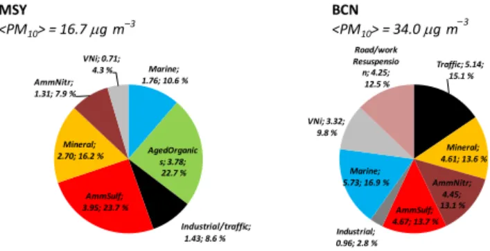
Figure 5. Source contributions from PMF model in PM10 at

Montseny (MSY) and Barcelona (BCN). Mean values during 2004–

2014. Values reported are sources in µg m−3_{and %.}

dust to PM10mass in the NE of Spain, and showed that the more negative the iNAO is, the lower the dust contribution to PM. The iNAO was unusually negative during the period 2008–2012 (http://www.cpc.ncep.noaa.gov/products/precip/ CWlink/pna/norm.nao.monthly.b5001.current.ascii), thus likely contributing to the explanation of the observed trends of crustal elements. Moreover, negative NAO can favor the presence of fronts that can sweep the Iberian Peninsula from west to east, causing stronger winds and less stagnant conditions, thus favoring the dispersion of pollutants. In addition, as suggested by Cusack et al. (2012), it could also be hypothesized that some part of the crustal material mea-sured at MSY is a product of the construction industry. The construction industry in Spain has been especially affected by the current economic recession, and crustal material pro-duced by this industry may have contributed to the crustal load in PM2.5. For example the number of home construction works in Barcelona during 2008–2014 (from the beginning of the economic crisis; mean number of works of 1281) reduced by around 75 % compared to the period 2000–2007 (mean number of works of 5187; http://www.bcn.cat/ estadistica/castella/dades/timm/construccio/index.htm). The fact that the total reduction calculated for mineral elements reported in Tables 2 and 3 was higher in PM2.5compared to PM10 could corroborate the hypothesis of an anthropogenic contribution to the mineral matter measured at MSY.

Finally, Na concentrations showed linear decreasing trends at both sites, with the exception of PM10Na at MSY. Other species at MSY such as OC and EC did not show statisti-cally significant trends. Consider that the concentrations of EC at MSY are very low and around an annual mean of 0.2– 0.3 µg m−3_{. Both anthropogenic activity and biomass} burn-ing were expected to contribute to this chemical species. Concerning OC, the lack of trend was probably due to the contribution from biogenic sources to the concentration of this species at regional level.

4 PMF source profiles and contributions

Eight and seven sources were detected at BCN and MSY, re-spectively, in PM10from PMF model. The absolute and rel-ative contributions of these sources to the measured PM10 mass were reported in Fig. 5, whereas the chemical pro-files of the detected sources were reported in the Supplement (Fig. S2).

Some sources were common at both BCN and MSY. These are secondary sulfate (secondary inorganic source traced by SO2₄−and NH+₄ and contributing 3.95 (23.7 %) and 4.67 µg m−3_{(13.7 %) at MSY and BCN, respectively),} sec-ondary nitrate (secsec-ondary inorganic source traced by NO−₃ and NH+₄ and contributing 1.31(7.9 %) and 4.45 µg m−3 (13.1 %) at MSY and BCN, respectively), V–Ni-bearing source (traced mainly by V, Ni, and SO2₄−, it represents the direct emissions from heavy oil combustion and contributed 0.71 (4.3 %) and 3.32 µg m−3_{(9.8 %) at MSY and BCN,} re-spectively), mineral (traced by typical crustal elements such as Al, Ca, Ti, Rb, and Sr and contributing 2.70 (16.2 %) and 4.61 µg m−3 _{(13.6 %) at MSY and BCN, respectively), and} aged marine (traced by Na and Cl mainly with contribu-tions from SO2₄− and NO−₃ and contributing 1.76 (10.6 %) and 5.73 µg m−3 _{(16.9 %) at MSY and BCN, respectively).} Sources detected at MSY but not at BCN were the indus-trial/traffic source (traced by EC, OC, Cr, Cu, Zn, As, Cd, Sn, Sb, and Pb), which included contributions from anthro-pogenic sources such as road traffic and metallurgic indus-tries and contributed 1.43 µg m−3_{(8.6 %), and aged organics} (traced mainly by OC and EC), with maxima in summer indi-cating mainly a biogenic origin and contributing 3.78 µg m−3 (22.7 %). The ratio OC : EC in the industrial/traffic and aged organic source profiles at MSY were 4.2 and 11.7, respec-tively, thus indicating a strong influence of aged particles in the latter source, with the former source being more fresh. The statistic of the OC : EC ratio based on chemical data at MSY is reported in the Supplement (Fig. S3). Mean and me-dian values of OC : EC ratio at MSY were 9.1 and 7.8, re-spectively.

Finally, some sources were detected at BCN but not at MSY: traffic (traced mainly by Cnm, Cr, Cu, Sb and Fe) contributing 5.14 µg m−3 _{(15.1 %), road/work resuspension} (traced by both crustal elements, mainly Ca, and traffic tracers such as Sb, Cu, and Sn) contributing 4.25 µg m−3 (12.5 %), and industrial/metallurgy (traced by Pb, Cd, As, and Zn) contributing 0.96 µg m−3_{(2.8 %).}

(13)

Table 4.Mann–Kendall and multi-exponential trends of source contributions in PM10from PMF at BCN (italic) and MSY. Type: linear (L),

single exponential (SE), double exponential (DE);a(µgm−3)andτ (yr) are the constants and the characteristic times, respectively, of the exponential data fittings; NL (%) is the nonlinearity; TR (%) is the total reduction; RC (%) is the residual component; ni denotes not included. Significance of the trends following the Mann–Kendall test:∗∗∗(pvalue < 0.001),∗∗(pvalue < 0.01),∗(pvalue < 0.05),+(pvalue < 0.1).

PM10(BCN; MSY) Mann–Kendall fit Multi-exponential fit

Source Contribution Contribution Fit NL pvalue Trend a τ Trend TR RC

2004 (µgm−3₎ _{2014 (µgm}−3₎ _type _{( %)} _(µgm−3_yr−1₎ _(µgm−3₎ _(yr) _(µgm−3_yr−1₎ _{( %)} _{( %)}

Secondary sulfate 10.27 3.38 DE 45 ∗∗

12.33 1.65 −0.71 67 16

3.82 105.80

6.57 3.07 SE 12 ∗∗

5.99 13.22 −0.32 53 21

Secondary nitrate 6.99 1.96 SE 14 ∗∗∗

8.54 8.96 −0.51 67 13

2.03 0.47 SE 15 ∗∗

2.44 8.59 −0.15 69 17

V–Ni-bearing 4.23 1.84 SE 11 ∗∗

5.66 10.59 −0.32 61 19

0.79 0.44 L 8 ∗∗ ₋

0.07 64 25

Industrial/metallurgy (BCN) 1.64 0.71 SE 21 ∗∗∗ _1.76 _9.56 ₋_0.10 ₆₅ ₁₆

Mineral ni ni

3.46 2.32 L 5 + −0.10 30 21

Industrial/traffic (MSY) 2.08 1.01 L 7 ∗∗ ₋

0.11 56 13

C

o

n

tr

ib

u

ti

o

n

[

m

g

m

]

3 _DE _SE _SE _SE

Secondary sulfate Secondary nitrate V-Ni bearing Industrial

–

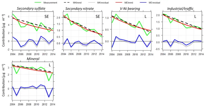
Figure 6. Mann–Kendall and multi-exponential trends for source contributions in PM10 at BCN. Measured concentration (green line);

multi-exponential trend (red line); multi-exponential residuals (blue line); Mann–Kendall trend (black line); Mann–Kendall residuals (gray line). Trend type: linear (L), single exponential (SE), double exponential (DE). The source contributions at BCN from mineral, traffic, and road/work resuspension were excluded from the trend discussion.

in Fig. SI-4, the relative differences in source contributions ranged from −3 % (Mineral source) to +20 % (industrial source), and R2 ranged from 0.894 to 0.997, thus confirm-ing the correct interpretation of the 2004–2014 PMF sources where Cnmwas used. The OC : EC ratio in the traffic source from 2007 to 2014 PMF was 1.70 (cf. Fig. S5), whereas the mean and median OC : EC ratios from chemistry data were 2.5 and 2.3, respectively, thus being in agreement with the contribution of fresh particles from the traffic source at BCN. 4.1 Trends of annual PM10source contributions

Figures 6 and 7 and Table 4 show the results from MK or ME tests applied to the annual averages of PM10source con-tributions at BCN and MSY. As already noted we cannot study trends for traffic, road/work resuspension, and min-eral source contributions at BCN because of the change of the station location in 2009. The contributions that showed statistically significant downward trends at both stations were from secondary sulfate, secondary nitrate, and V–Ni-bearing sources (p< 0.001 orp< 0.01). Moreover,

statisti-cally significant decreasing trends were observed for the in-dustrial/traffic (p< 0.01) and mineral (p< 0.1) source con-tributions at MSY and for the industrial/metallurgy source contribution (p< 0.001) at BCN. These sources were mostly linked with anthropogenic activities, and the observed de-creasing trends confirmed the effectiveness of pollution con-trol measures together with the possible effect of the eco-nomic crisis in Spain from 2008. Conversely, the contribu-tions from sources mostly linked with natural processes such as aged marine (at both BCN and MSY) and aged organic (at MSY) did not show statistically significant trends.

(14)

C

o

n

tr

ib

u

ti

o

n

[

m

g

m

]

3

SE SE L L

Secondary sulfate Secondary nitrate V-Ni bearing Industrial/traffic

Mineral

C

o

n

tr

ib

u

ti

o

n

[

m

g

m

]

3 L

–

Figure 7.Mann–Kendall and multi-exponential trends for source contributions in PM10at MSY. Measured concentration (green line);

multi-exponential trend (red line); multi-multi-exponential residuals (blue line); Mann–Kendall trend (black line); Mann–Kendall residuals (gray line). Trend type: linear (L), single exponential (SE), double exponential (DE).

mostly from power generation (MAGRAMA, 2013; Querol et al., 2014). In BCN the two characteristic times (one low and the other high, cf. Table 4) of the DE fit indicated a strong decrease of the secondary sulfate source contribution at the beginning of the period. This decrease was sharper compared to MSY where the SE fit was used. This differ-ence was mostly due to the ban of heavy oils and petroleum coke for power generation around Barcelona from 2007. The effects of this AQ regional plan were likely more visible in BCN compared to MSY, thus explaining the two differ-ent expondiffer-ential fits used. Overall, for the secondary sulfate source contributions, the TRs were rather high around 53 at MSY and 67 % at BCN, with RC ranging from 16 (BCN) to 21 % (MSY). The fact that the trend of the secondary sulfate source contribution was exponential likely suggested the at-tainment of a lower limit, and indicated a limited scope for further reduction of SO2 emissions in our region. In fact, it has been estimated that the maximum in EU will be a further 20 % reduction through measures in industry, residential and commercial heating, and reduced agricultural waste burning (UNECE, 2016). Conversely, in eastern European countries the scope for reduction is much greater and around 60 % (UNECE, 2016).

The trends of the secondary nitrate source contribu-tions were SE at both stacontribu-tions with very similar τ (8.96– 8.59 years), TR (67–69 %), and RC (13–17 %). The decrease observed for the contribution from the secondary nitrate source was related to the reduction in ambient NOx

concen-trations (Figs. 8 and 9). Figure 9 shows the levels of tropo-spheric NO2column from 2005 to 2014 in southern Europe

from NASA NO2Ozone Monitoring Instrument (OMI) Level 3 plotted using the Giovanni online data system (Acker and Leptoukh, 2007). In Spain, a general decrease of the concen-trations of columnar NO2at regional level can be observed. Overall, the implementation of European directives affect-ing industrial and power generation emissions as well as the increase of the proportion of energy produced from renew-able sources (cf. Fig. 10 for Spain), among others, produced a significant reduction of SO2 and NOx emissions. Around

Barcelona the observed decreases were also attributed to the decrease of NOxemissions, mainly from the five power

gen-eration plants around the city. Moreover, the implementation of the regional AQ Plan for SCRT (continuously regenerating PM traps with selective catalytic reduction for NO2)and the hybridization and shift to natural gas engines of Barcelona’s bus fleet may have had an influence in the observed reduc-tions.

(15)

%

Y

ear

Figure 8.Spanish national emission of SO2and NOx(normalized

to year 2004).

The industrial/metallurgy source contribution at BCN de-creased exponentially (SE) at the rate of−0.10 µg m−3_yr−1 (p< 0.001), reflecting the SE decreasing trends observed for the main tracers of this pollutant source (Pb, Cd, and As; cf. Table 2). The decrease of industrial emissions was mainly attributed to the implementation of the IPPC (Integrated Pol-lution Prevention and Control) Directive. Moreover, the ob-served decrease may be attributed to a decrease in the emis-sions from industrial production (smelters; Querol et al., 2007) at a regional scale around Barcelona. Also, the finan-cial crisis, whose impact on industrial production and use of fuels has been evident since October 2008 also contributed to the observed trend. TR and RC for the industrial source contributions at BCN were 65 and 16 %, respectively. As for the contributions from secondary sulfate and nitrate sources, the exponential trend observed for the industrial/metallurgy source contribution suggested the attainment of a lower limit. As evidenced in Fig. 6, the contribution from this source from 2010 was quite low and rather constant.

The contribution of the industrial/traffic source at MSY showed similar magnitude of the trend (−_{0.11 µg m}−3_yr−1 with p< 0.01) compared to the BCN industrial/metallurgy contribution, both sources being traced mostly by the same industrial tracers. However, this source at MSY was also traced by traffic tracers (i.e., Cu and Sn), which decreased linearly with time (cf. Table 2), thus likely explaining the lin-ear trend observed for the contribution of this source at MSY. TR and RC were 56 and 13 %, respectively, similar to those calculated for the industrial source contribution at BCN.

Finally, the mineral source contribution at MSY showed linear slightly significant decreasing trend (p< 0.1) in agree-ment with that observed at the same station by Cusack et al. (2012). As already noted in Sect. 3.3, this negative trend could be due to both a possible decrease of the emissions of finer anthropogenic mineral species from specific sources, such as cement and concrete production and construction works, and unusual weather conditions, reducing the Saha-ran dust contribution to PM and resuspension of dust.

In order to further interpret the observed trends, annual data on the annual National Energy Consumption (NECo) from different energy sources (MINETUR, 2013) were also evaluated (Fig. 10). Overall, the primary energy consump-tion in Spain (NECo statistical data for Spain-MINETUR, 2013) increased from 2004 to 2007 and decreased from 2007, with a marked decrease in 2009. From 2009, the energy con-sumption indicator remained rather low and constant until 2012, when an additional decrease in 2013 and 2014 was ob-served. Oil consumption was fairly constant during 2004– 2007, showing an important decrease during 2008–2014. This trend was probably governed by the fuel consumption for traffic road. Coal consumption remained constantly high from 2004 to 2007, whereas, as for the emissions of SO2 (Fig. 8), a sharp decrease occurred from 2007. However, in the period 2011–2014, there was an important increase of coal consumption leading to an average consumption simi-lar to the year 2008. However, the implementation of FGD systems contributed to maintain SO2at low concentrations, even in the coal production regions in Spain (cf. Querol et al., 2014). The hydroelectric generation was rather specular to coal consumption. For example, the increase in 2010 of hydroelectric consumption, due to high rainfall rate, mirrored the decrease in the coal consumption observed the same year. Finally, renewable energy consumption increased by 440 % from 2004 to 2014, with a gradual growth in the NECo.

5 Conclusions

(16)

2005 2006

2007 2008

2009 2010

2011 2012

2013 2014

Mean annual tropospheric NO2column

(clear, 0–30 % cloud)

(1014molec _{cm )}_–2

Figure 9.NASA OMI Level 3 tropospheric NO2column plotted using the Giovanni online data system, developed and maintained by the

NASA GES DISC.

Figure 10. Annual (2004–2014) energy consumption for Spain (normalized to year 2004). Data from the Spanish Ministry of In-dustry (MINETUR, 2013).

in vehicle brakes. Secondary inorganic aerosols (SO2−

4 , NO

−

3 and NH+₄)also showed marked decreasing trends (both linear and exponential) in both fractions and at both sites. However, in general the magnitude of the trends for these species and

their statistical significance were higher at BCN compared to MSY.

(17)

such as aged marine (at both BCN and MSY) and aged or-ganic (at MSY) did not show statistically significant trends. The general trends observed for the calculated PMF source contributions reflected the trends observed for the chemi-cal tracers of these pollutant sources well. The decrease in the secondary sulfate source contribution was mainly at-tributed to the EC Directive on Large Combustion Plants implemented in Spain from 2008, resulting in the applica-tion of flue gas desulfurizaapplica-tion (FGD) systems in a num-ber of large facilities. Moreover, according to the 2008 re-gional AQ plan, the use of heavy oils and petroleum coke for power generation was forbidden around Barcelona from 2008 in favor of natural gas. As a consequence, a decrease of the contributions from the V–Ni-bearing source at both sites was also observed. The decrease observed for the contribu-tion of the secondary nitrate source was mainly due to the reduction in ambient NOxconcentrations. In Spain a general

decrease of the concentrations of NO2at regional level was observed, and it was mainly related with the lower energy consumption related with the financial crisis. The decrease of nitrates concentrations and secondary nitrate source contri-butions around Barcelona was also attributed to the decrease of NOx emissions from the five power generation plants

around the city. Moreover, a regional AQ plan implementing the SCRT (continuously regenerating PM traps with selec-tive catalytic reduction for NO2)and the hybridization and shift to natural gas engines of Barcelona’s bus fleet may have also had an influence on NOx ambient concentrations. The

industrial/metallurgy source contribution at BCN decreased exponentially, reflecting the exponential trends observed for the main tracers of this pollutant source (Pb, Cd and As). The implementation of the IPPC (Integrated Pollution Preven-tion and Control) Directive, together with a decrease in the emissions from industrial production (smelters) at a regional scale around Barcelona, explained the observed trends. Over-all, the magnitudes of the decreasing trends of the contribu-tions of the pollutant sources were higher at BCN compared to MSY, likely because of the proximity of the BCN mea-surement site to anthropogenic pollutant sources compared to the MSY site. The results presented in this work clearly confirm the beneficial effect of the AQ measures taken in recent years in Europe. However, the WHO limit values of specific pollutants, such as PM10 and PM2.5, are still ex-ceeded, especially at urban level and industrial hotspots. To meet the WHO guide levels, important action is still required for the next decade and the interpretation of past air qual-ity trends may yield relevant outcomes for planning further cost-effective actions. We would like to highlight that a non-linear approach to trend studies is very attractive, given that some air pollutants reported in this work showed reductions that are not gradual with time. Conversely, for specific pollu-tant source-contribution/concentration in our region, the de-creasing trends were less steep at the end of the period com-pared to the beginning, thus likely indicating the attainment of a lower limit. This was the case, for example, for the

sec-ondary sulfate source contribution decreasing exponentially from 2004 to 2014, thus likely indicating a limited scope for further reduction of SO2emissions in our region.

6 Data availability

The Montseny data sets used for this publication are accessi-ble online on the following web page: www.http://ebas.nilu. no/. The Barcelona data sets were collected within different national/regional projects and/or agreements and are avail-able upon request.

The Supplement related to this article is available online at doi:10.5194/acp-16-11787-2016-supplement.

Acknowledgements. This work was supported by the MINECO (Spanish Ministry of Economy and Competitiveness), the MAGRAMA (Spanish Ministry of Agriculture, Food and Envi-ronment), the Generalitat de Catalunya (AGAUR 2014 SGR33 and the DGQA), and FEDER funds under the PRISMA project (CGL2012-39623-C02/00). The research leading to these results has received funding from the European Union’s Horizon 2020 research and innovation programme under grant agreement no. 654109 and previously from the European Union Seventh Framework Programme (FP7/2007-2013) under grant agreement no. 262254. Marco Pandolfi is funded by a Ramón y Cajal Fellowship (RYC-2013-14036) awarded by the Spanish Ministry

of Economy and Competitiveness. NO₂map analyses and

visual-izations used in this paper were produced with the Giovanni online data system, developed and maintained by the NASA GES DISC. The authors would like to express their gratitude to D. C. Carslaw and K. Ropkins for providing the Openair software used in this paper (Carslaw and Ropkins, 2012; Carslaw, 2012).

Edited by: V.-M. Kerminen

Reviewed by: three anonymous referees

References

Acker, J. G. and Leptoukh, G.: Online Analysis Enhances Use of NASA Earth Science Data, Eos, Trans. AGU, 88, 14–17, 2007. Alastuey, A., Minguillón, M. C., Pérez, N., Querol, X., Viana, M.,

and de Leeuw, F.: PM10 Measurement Methods and Correc-tion Factors: 2009 Status Report, ETC/ACM Technical Paper 2011/21, 2011.

Amato, F., Pandolfi, M., Escrig, A., Querol, X., Alastuey, A., Pey, J., Perez, N., and Hopke, P. K.: Quantifying road dust resuspension in urban environment by Multilinear Engine: A comparison with PMF2, Atmos. Environ., 43–17, 2770–2780, 2009.

Barmpadimos, I., Keller, J., Oderbolz, D., Hueglin, C., and

Prévôt, A. S. H.: One decade of parallel fine (PM₂_.₅) and

coarse (PM10-PM2.5) particulate matter measurements in

(18)

Carslaw, D. C.: The OpenAir manual – open-source tools for analysing air pollution data, Manual for version 0.5–16, King’s College, London, 2012.

Carslaw, D. C. and Ropkins, K.: OpenAir – an R package for air quality data analysis, Environ. Model Softw., 27–28, 52–61, 2012.

Cavalli, F., Viana, M., Yttri, K. E., Genberg, J., and Putaud, J.-P.: Toward a standardised thermal-optical protocol for measuring atmospheric organic and elemental carbon: the EUSAAR proto-col, Atmos. Meas. Tech., 3, 79–89, doi:10.5194/amt-3-79-2010, 2010.

Cusack, M., Alastuey, A., Pérez, N., Pey, J., and Querol, X.: Trends of particulate matter (PM2.5) and chemical composition at a

re-gional background site in the Western Mediterranean over the last nine years (2002–2010), Atmos. Chem. Phys., 12, 8341–8357, doi:10.5194/acp-12-8341-2012, 2012.

EEA: European Environmental Agency Air quality in Eu-rope – 2013 report, EEA report 9/2013, Copenhagen, 1725–9177, available at: http://www.eea.europa.eu/publications/ air-quality-in-europe-2013 (last access: 10 March 2016), 2013. EEA: European Environmental Agency Air quality in Europe

– 2015 report, Many Europeans still exposed to harmful air pollution, Air pollution is the single largest environmental health risk in Europe, EEA report 11/2015, Copenhagen, 1– 7, available at: http://www.eea.europa.eu/media/newsreleases/ many-europeans-still-exposed-to-air-pollution-2015 (last ac-cess: 16 May 2016), 2015.

Escrig, A., Monfort, E., Celades, I., Querol, X., Amato, F., Min guil-lon, M. C., and Hopke, P. K.: Application of optimally scaled tar-get factor analysis for assessing source contribution of ambi ent PM10, J. Air Waste Manage., 59, 1296–1307, 2009.

Gilbert, R. O.: Statistical Methods for Environmental Pollution Monitoring, Wiley, NY, 1987.

Guerreiro, C., Leeuw, F. de, Foltescu, V., Horálek, J., and European Environment Agency: Air quality in Europe 2014 report, Luxem-bourg: Publications Office, available at: http://bookshop.europa. eu/uri?target=EUB:NOTICE:THAL14005:EN:HTML (last ac-cess: 2 June 2016), 2014.

Harrison, R. M., Stedman, J., and Derwent, D.: New directions: why are PM10 concentrations in Europe not falling?, Atmos. Envi-ron., 42, 603–606, 2008.

Henschel, S., Querol, X., Atkinson, R., Pandolfi, M., Zeca, A., Le Tertre, A., Analitis, A., Katsouyanni, K., Chanel, O., Pascal, M., Bouland, C., Haluza, D., Medina, S., and Goodman, P. G.: Am-bient air SO2patterns in 6 European cities, Atmos. Environ., 79,

236–247, 2013.

Henschel, S., Le Tertre, A., Atkinson, R.W., Querol, X., Pandolfi, M., Zeka, A., Haluza, D., Antonis, A., Katsouyanni, K., Bouland, C., Pascal, M., Medina, S., and Goodman, P. G.: Trends of nitro-gen oxides in ambient air in nine European cities between 1999 and 2010, Atmos. Environ., 117, 234–241, 2015.

Kendall, M. G.: Rank Correlation Methods, 4th Edn., Charles Grif-fin, London, 1975.

MAGRAMA: Inventario Nacional de Emisiones de Contami-nantes a la Atmósfera, Ministerio de Agricultura, Alimentación y Medio Ambiente del Gobierno de España, available at: http://www.magrama.gob.es/ca/calidad-y-evaluacion-ambiental/

temas/sistemaespanol-de-inventario-sei-/ (last access: 12

February 2016), 2013.

Mann, H. B.: Non-parametric tests against trend, Econometrica, 13, 163–171, 1945.

MINETUR: Ministerio de Industria, Energía y Turismo, Go-bierno de España: energy statistics and balances, avail-able at: http://www.minetur.gob.es/energia/balances/Balances/ Paginas/CoyunturaTrimestral.aspx (last access: 12 February 2016), 2013.

Paatero, P.: Least squares formulation of robust non-negative factor analysis, Chemometr. Intell. Lab., 37, 23–35, 1997.

Paatero, P.: User’s guide for positive matrix factorization pro-grams PMF2 and PMF3, Part 1: tutorial, University of Helsinki, Helsinki, Finland, 2004.

Paatero, P. and Tapper, U.: Positive Matrix Factorization: a non neg-ative factor model with optimal utilization of error estimates of data values, Environmetrics, 5, 111–126, 1994.

Paatero, P. and Hopke, P. K.: Discarding or downweighting high noise variables in factor analytic models, Anal. Chim. Ac., 490, 277–289, doi:10.1016/s0003-2670(02)01643-4, 2003.

Paatero, P., Hopke, P. K., Song, X., and Ramadan, Z.: Under-standing and controlling rotations in factor analytic models, Chemometr. Intell. Lab., 60, 253–264, 2002.

Paatero, P., Hopke, P. K., Begum, B. A., and Biswas, S. K.: A graph-ical diagnostic method for assessing the rotation in factor analyt-ical models of atmospheric pollution, Atmos. Environ., 39, 193– 201, doi:10.1016/j.atmosenv.2004.08.018, 2005.

Pandolfi, M., Cusack, M., Alastuey, A., and Querol, X.: Variability of aerosol optical properties in the Western Mediterranean Basin, Atmos. Chem. Phys., 11, 8189–8203, doi:10.5194/acp-11-8189-2011, 2011.

Pandolfi, M., Amato, F., Reche, C., Alastuey, A., Otjes, R. P., Blom, M. J., and Querol, X.: Summer ammonia measurements in a densely populated Mediterranean city, Atmos. Chem. Phys., 12, 7557–7575, doi:10.5194/acp-12-7557-2012, 2012.

Pandolfi, M., Martucci, G., Querol, X., Alastuey, A., Wilsenack, F., Frey, S., O’Dowd, C. D., and Dall’Osto, M.: Continuous at-mospheric boundary layer observations in the coastal urban area of Barcelona during SAPUSS, Atmos. Chem. Phys., 13, 4983– 4996, doi:10.5194/acp-13-4983-2013, 2013.

Pandolfi, M., Querol, X., Alastuey, A., Jimenez, J. L., Jorba, O., Day, D., Ortega, A., Cubison, M. J., Comerón, A., Sicard, M., Mohr, C., Prévôt, A. S. H., Minguillón, M. C., Pey, J., Bal-dasano, J. M., Burkhart, J. F., Seco, R., Peñuelas, J., van Drooge, B. L., Artiñano, B., Di Marco, C., Nemitz, E., Schallhart, S., Metzger, A., Hansel, A., Lorente, J., Ng, S., Jayne, J., and Szi-dat, S.: Effects of sources and meteorology on particulate mat-ter in the Wesmat-tern Medimat-terranean Basin: An overview of the DAURE campaign, J. Geophys. Res.-Atmos., 119, 4978–5010, doi:10.1002/2013JD021079, 2014.

Pérez, N., Pey, J., Castillo, S., Viana, M., Alastuey, A., and Querol, X.: Interpretation of the variability of levels of regional back-ground aerosols in the Western Mediterranean, Sci. Total Envi-ron., 407, 527–540, doi:10.1016/j.scitotenv.2008.09.006, 2008. Pey, J., Pérez, N., Querol, X., Alastuey, A., Cusack, M., and

Reche, C.: Intense winter atmospheric pollution episodes affect-ing the Western Mediterranean, Sci. Total Environ., 408, 1951–9, doi:10.1016/j.scitotenv.2010.01.052, 2010.