entropy 2013, 15, 1609-1623; doi:10.3390/e15051609
entropy
ISSN 1099-4300 www.mdpi.com/journal/entropy Article
A Novel Nonparametric Distance Estimator for Densities with
Error Bounds
Alexandre R.F. Carvalho 1,*, João Manuel R. S. Tavares 1 and Jose C. Principe 2
1 Instituto de Engenharia Mecânica e Gestão Industrial, Faculdade de Engenharia, Universidade do Porto; Rua Dr. Roberto Frias, s/n 4200-465 Porto, Portugal; E-Mail: [email protected]
2 Computational Neuro Engineering Laboratory, University of Florida; EB451 Engineering Building, University of Florida, Gainesville, FL 32611, USA; E-Mail: [email protected]
* Author to whom correspondence should be addressed; E-Mail: [email protected]; Tel.: +351-225-081-719; Fax: +351- 225-081-440.
Received: 19 December 2012; in revised form: 25 April 2013 / Accepted: 28 April 2013 / Published: 6 May 2013
Abstract: The use of a metric to assess distance between probability densities is an important practical problem. In this work, a particular metric induced by an α-divergence is studied. The Hellinger metric can be interpreted as a particular case within the framework of generalized Tsallis divergences and entropies. The nonparametric Parzen’s density estimator emerges as a natural candidate to estimate the underlying probability density function, since it may account for data from different groups, or experiments with distinct instrumental precisions, i.e., non-independent and identically distributed (non-i.i.d.) data. However, the information theoretic derived metric of the nonparametric Parzen’s density estimator displays infinite variance, limiting the direct use of resampling estimators. Based on measure theory, we present a change of measure to build a finite variance density allowing the use of resampling estimators. In order to counteract the poor scaling with dimension, we propose a new nonparametric two-stage robust resampling estimator of Hellinger’s metric error bounds for heterocedastic data. The approach presents very promising results allowing the use of different covariances for different clusters with impact on the distance evaluation.
Keywords: generalized differential entropies; generalized differential divergences; Tsallis entropy; Hellinger metric; nonparametric estimators; heterocedastic data
PACS Codes: 02.50.-r, 02.50.Cw, 89.70.-a, 89.70.Cf
1. Introduction
Distances measures between two probability densities have been extensively studied in the last century [1]. These measures address two important main objectives: how difficult it is to distinguish between one pair of densities in the context of others and to assess the closeness of two densities, compared to others [2]. In learning scenarios essentially associated with the test of a single hypothesis, the use of a divergence to represent the notion of distance is efficient. However, in scenarios involving multiple hypotheses, such as clustering, image retrieval, or pattern recognition and signal detection, for instance, the non-symmetric and non-metric nature of divergences becomes problematic [3]. When deciding the closest or the farthest among three or more clusters, the use of a metric is important. In this work, a novel nonparametric metric estimator for densities with error bounds is presented. Shannon’s entropy has a central role in information-theoretic studies. However, the concept of information is so rich that perhaps there is no single definition that will be able to quantify information properly [4]. The idea of using information theory functional, such as entropies or divergences, in statistical inference is not new. In fact, the so-called statistical information theory has been the subject of much research over the last half century [5]. How to measure the distance between two densities is an open problem with several proposals since the work of Hellinger in 1909 with Hellinger’s distance [1], Kullback and Leibler (1951), with Kullback-Leibler’s divergence [6], Bregman (1967) with the Bregman’s divergence [7], Jeffreys (1974) with J-distance [8], RAO (1985) and Jianhua Lin (1991) with Jensen-Shannon’s divergence [9,10], Menéndez et al. (1997) with (h, Φ)-entropy differential metric [11], Seth and Principe (2008) with correntropy [12], among others. This work looks into Hellinger’s metric that is the preferred [13,14] or natural model metric [15]. In 2007 Puga found that Hellinger’s metric is one particular α-divergence [16]. Here, we propose a new measure change to solve the nonparametric metric estimation and a two stage robust estimator with error bounds.
2. Theory Background
Following Hartley’s (1928) and Shannon’s (1948) works [17,18], Alfred Rényi introduced in 1960 the generalized α-entropy [19] of probability density functionf
x :
f x dx f R ln 1 1 , α (1) The corresponding generalized differential divergence between two densities f1
x and f2
x is:
1 1 2 1 2 1 , ln 1 R f x D f f dx f x
(2)Gell-Mann and Tsallis considered another family of α-entropies [20]:
f x dx f T 11 1 (3) being the corresponding α-divergences given as:
1 1 2 1 2 1 , 1 1 T f x D f f dx f x
(4)Entropy 2013, 15 1611 Making 1, one easily can conclude that:
f T
f H
f R S 1 lim1 lim (5) and:
1 2
1 2
1 2
1 1 lim R , lim T , , KL D f f D f f D f f (6) where:
f
f
x f
x dx HS ln (7)is Shannon’s differential entropy and:
dx x f x f x f f f DKL 2 1 1 2 1, ln (8) is Kulback-Leibler’s divergence.Another member of these families is the Rényi’s quadratic entropy (α=2) that is defined as:
f
f
x dxR2 ln 2 (9)
while the respective divergence is:
1
2 2 1 2 2 , ln R f x D f f dx f x
(10)Rényi’s quadratic entropy, given by Equation (9), is particularly interesting because it accepts a close form nonparametric estimator, saving computational time compared to numerical integration or resampling [21,22].
α-Entropy families given by Equations (1) and (3) are monotonically coupled (Ramshaw [23]) through:
1 R 1
1
T e
(11)
Therefore, an optimization in one family has equivalence in the other. 2.1. Square-Root Entropy
Let us consider
1 2 in Equations (1)–(4). Then, the square-root entropy in the form of Tsallis is:
1 2 2 2
T f
f x dx (12)with the corresponding divergence given as:
1 2 1, 2 2 2 1 2
T
D f f
f x f x dx (13)In Rényi’s form one finds, respectively, the entropy:
1 2 2 ln ,
R f
f x dx (14)and the divergence:
1 2 1, 2 2 ln 1 2
R
D f f
f x f x dx (15)
1 2
2 2 1 2 1 2 1 f , f f x f x dx M f , f DT
(16)where M
f1, f2
is a information theoretic derived metric that, among other properties, verifies the triangular inequality. This particular -divergence, by means of a monotonous transformation, induces the Hellinger’s distance, which is a metric [13,14,24]:
1, 2
2 2 ( , )1 2M f f I f f (17)
On the other hand, information theoretic derived metrics given by Equations (15) and (16) are also related with Hellinger’s affinity or Bhattacharya’s coefficient (0I
f1,f2
1):
1, 2
1
2 .I f f
f x f x dx (18)Considering the expected cross-value of two probability density functions C
f1, f2
:
1, 2
f1
2 f2
1 1
2C f f E f E f
f x f x dx (19)the Hellinger’s affinity given by Equation (18) can be then written as:
1, 2
1, 2
1, 2
I f f C f f
f x dx C f f H f (20)where f
x is the normalized product density:
1
2
1, 2 f x f x f x C f f (21)and H
f the corresponding entropy of the information theoretic derived metric.This metric has bounds that can be directly computed from the samples as shown by Puga [16]. These bounds often present overlapping hypothesis intervals, and resampling estimation is a necessary tool to remove ambiguities and access distances between densities.
2.2. Nonparametric Hellinger’s Affinity Estimation
Let us focus on the application of the previous measures on two Parzen’s nonparametric densities [25] from two data clusters
2 1 1
1 1 ) 1 ( 1 ,..., ,x xN x Cl and
2 2 2
2 1 ) 2 ( 2 ,..., ,x xN x Cl :
1 1 1 1 1 1 , , 1 N j j x x G N x f (22) and:
2
2 2 2 1 2 1 , , N j j f x G x x N
(23)where G
x,
,
is the Parzen’s Gaussian kernel, also known as kernel bandwidth, with the approximation of covariance 2I, and mean given as:
2 2 ( ) 2 2 1 1 , , 2 x i i i G x e
(24)Entropy 2013, 15 1613 where is the dimension. Notice that the two clusters in Equations (22) and (23) may have two different Gaussian kernel covariances. The kernel covariance may be obtained directly from the a priori knowledge of the instruments used to produce the data; for instance, two different instruments with different precisions may produce the same data, but the densities should reflect the measurements error through the bandwidth, (covariances). To estimate the bandwidth without instrumental apriori knowledge it is possible to estimate the kernel bandwidth with a suitable method, such as k-Nearest Neighbor (k-NN), Silverman [25] or Scott [26].
Now, let us adopt the summing convention
1 2 1 1 , N i N j j i
and define the following auxiliary variables:
2 2 2 1 2 2 (25) 2 2 2 2 * 1 2 2 (26)
2 1 2 2
2 , 2 1 2 i j i j s x x (27)
1 2
2 ,j i j i x x d (28) and:
2 2 , , 2 2 , , i j k l d d D i j k l F d e
e (29)The nonparametric estimator fˆ
results in:
2
, * , , ˆ , , D i j i j i j f
F d G s (30)2.3. The Resampling Estimator
The bootstrap resampling is reached through the distribution of probability given by Equation (30) combined with the random generation of samples
k from nonparametric Parzen’s density with diagonal covariance, which is a well-established as well as a computationally efficient procedure [27]. Then, the synthesized samples are directly usable in the estimator:
1
1 1 1 lim lim ˆ K f K K K k k f H f f d d f E H f K f f
(31) with f d i i k .~. . .However, the use of Equation (31) is associated with serious practical difficulties because the second moment:
2dH f
has infinite variance, which is a condition where the central limit theorem is not valid. In this work, we use measure theory and propose the following change of measure:
z f (33)
with the associated density fZ(z):
max 0 ) ( ˆ 1 lim 1 1 k Z z k z k K f f f z dz z z E f E with zki.i~.d.fZ (34)This new density presents a finite second moment:
max 2 0 1 ( ) z z f z dz H f z
(35)having fz a limited support between 0 (zero) and zmax. This is a density with an abrupt jump in zmax
end of the density. However, the approximation properties of a histogram are not affected by a simple jump at the end of the density [26], hence the histogram estimator was used to estimate fˆZ(zk) with
.
The product probability density function
fz must be estimated from the random variable
f
z , but it ensures finite variance, which is a requisite of the central limit theorem and the t-student confidence interval may be used Equation (39).
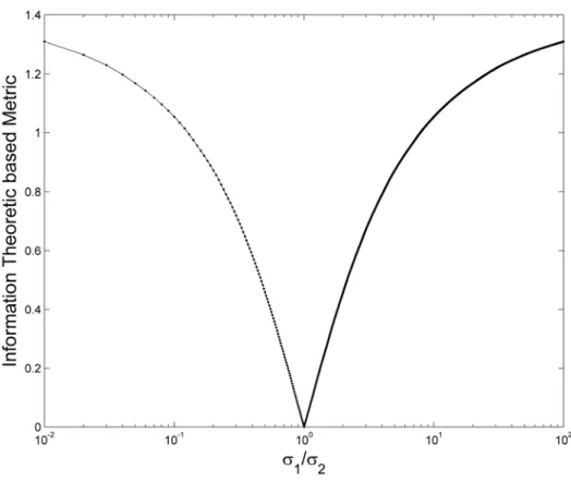
Figure 1. A logarithmic scale for the
1/
2 coefficient variation and metric measure change between the two respective densities
f1, f2
.
k k f z ˆ Entropy 2013, 15 1615 To test the algorithm, we consider the simplest case of Hellinger’s metric (17) associated with the nonparametric densities of Equations (22) and (23). In this particular case, we have access to the analytical value of Hellinger’s metric:
2 1,2 2 2 1 2 1 2 2 2 1 2 2 , 2 2 d M f f e (36)Using Equations (34) and (36), we can quantify the computational behavior of the resampling estimator. Let us first consider the behavior of the Parzen’s density estimator with two distinct kernel sizes: 1, 2. In the simplest case with only two kernels, located at the same coordinates, despite the same location, different Parzen’s windows in Equation (36) provide different distances, as can be observed in Figure 1. It is possible to verify the symmetric behavior of the distance estimator and realize that the bandwidth of the Parzen’s kernel is important to access the distance between clusters. This is a relevant characteristic, especially when the experimental data have different instrumental origins with different measurement precisions; the use of different bandwidths in the Parzen’s kernels may reflect this importance feature of the density, and this implies that the data is heterocedastic.
To quantify the error bounds estimation performance, we propose the generation of N1 distance
samples M~m from resampling the density of Equation (34), and to estimate f~Z we use a discrete histogram with N1 bins, obtaining the ordered z and k fZk
~
. As such, the metric estimator becomes:
1 ~ 1 2 1... 1 2 2 , ( ) m Z k k m N M C f f f z z z (37) which can be written as:
max ~ 1 2 0 1 2 2 , k ( ) z k Z k M C f f f z z z
(38)To assess the error bounds estimation, we use the t-student 95% confidence interval (39), which is a maximum entropy distribution [28,29] and provides a parametric approach to robust statistics [30], and allows the following calculation of the confidence limits:
1
1 2 1,0.5 0.95/2 1 1 1 1 , ( 1) N N m k L U M t M M N N
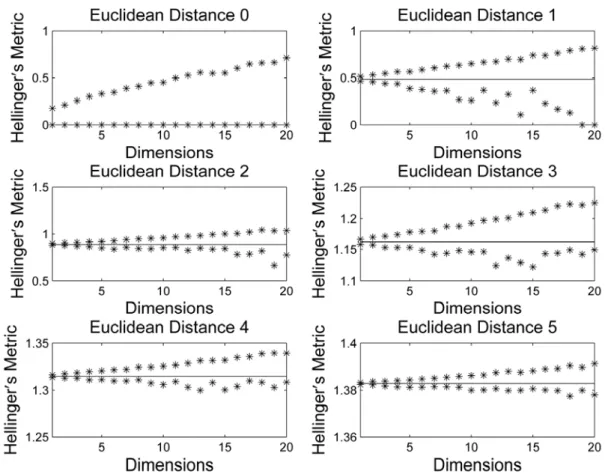
(39)We calculate the 95% confidence limits, the upper (U ) and the lower (L) for the respective density resampling. The variance of this new estimator is well controlled in one dimension. The unexpected drawback of this estimator is its poor scaling performance with increased dimension, as depicted in Figure 2.
The new variable z f
may be seen as a projection of the multidimensional Parzen’s kernels into a 1-Dimensional function. This insight allowed the design of a two-stage estimator for f
that circumvents both problems: infinite variance and poor scalability with dimensionality.Figure 2. Illustration of the metric estimator behavior for dimensions 1 (one) to 5.
2.4. The Two Stage Resampling Estimator
We propose the generation of N1 distance samples M~k(n) from resampling the density f(k), which constitutes one trial )(n :
1 1 2 ( ) ( ) 1 ... , 2 2 n k n k k N C f f M f (40) It is possible to estimate M as: ~(n)
1 1 2 ( ) ( ) 1 1 , 2 2 N n n k k C f f M N f
(41)For each trial )(n , the 95% confidence limits, the upper U (n)and the lower L(n) for the respective
density resampling, can be calculated:
1 1 2 ( ) ( ) ( ) ( ) ( ) 1,0.5 0.95/ 2 1 1 1 1 , ( 1) N n n n n n N k k L U M t M M N N
(42)It may seem that this step is enough to estimate the metric M~
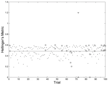
f1,f2
22~I(f1,f2), but the theoretically predicted undesired behavior associated to Equation (32), with large confidence intervals is present in this estimator. To demonstrate this drawback, we have simulated 100 trials of the simplest case of nonparametric Hellinger’s metric, Equation (36), with Euclidean distanced x1x2 1. As can be observed in Figure 3, the large confidence intervals are present, hence the motivation for the two-stage error bound estimator.Entropy 2013, 15 1617 Figure 3. t-Student 95% confidence intervals for Hellinger’s metric defined by dots; the exact value is represented by a continuous line; the predicted large intervals are marked with triangles; and the miss-estimated intervals are marked with circles.
To achieve a robust error bound estimator
LR UR
~ , ~
for the expected value of M(f1,f2) with similar results of fZ(z) in one dimension, we propose a new two-stage method. Comparing the results of the two densities resampling, we found that 31 selected trials out of 33 from fˆ(k) was in good agreement with ~fZ(z). With 33 trails )(n generated with N1 random samples each as:
1 1 2 ( ) 1 ... 1 ...3 3 , 2 2 ˆ n k k N n C f f f (43) sorting the amplitude U(n) L(n) and keeping the 31 smallest intervals with the correspondentestimated affinities (M~s(n)), we obtain the estimator for the second stage with:
31 ( ) 1 2 1 1 ( , ) 31 n s s n M f f M
(44)Then, we calculated the respective t-student 95% confidence interval
Ls Us
~ , ~
with the selected trials
) (
ˆ n s
M . To overcome the miss-estimated intervals, we have defined a second estimator for the lower limit of the interval (L~2) and a second estimator for the upper limit of the interval (U~2):
31 31 ( ) ( ) 2 2 1 1 1 1 , , 31 31 n n s s n n L U L U
(45)which is a potentially asymmetric interval, guided by the selected first-stage interval limits.
The robust estimator for the lower limit of the interval (L~R) and the robust estimator for the upper limit of the interval (UR
~
) were defined as:
2
2
, min , , max , R R s s L U L L U U (46) ) , ( ~ 2 1 f f MsIn Figure 4, we can find the intervals defined by Equation (46), and confirmed the robust interval estimator for the Hellinger’s affinity.
Figure 4. Using the new robust two-stage resampling interval estimator the exact Hellinger’s distance is more likely to be found within the interval; it should be noted that from dimension 1 to dimension 20, the exact value of the metric is always in the interval.
The detailed process of the two-stage estimator is presented in Algorithm 1. Notice that we studied up to dimension 20 with promising results. k-NN is a good alternative [31–36], but may present several difficulties, like the k determination [37], the distance measure choice [38] and the curse of dimensionality [39].
Algorithm 1—Two-stage resampling estimator
(1) COMMENT [To find the bandwidth of a cluster.
Use the apriori knowledge from the instrumental data to estimate the bandwidth.
If the precision of the instrumental data is not available, then use one of the preferred method to estimate bandwidth [26]; here it is used the Silverman rule and a cross validation search for maximum likelihood density [25].
(2) COMMENT [To estimate one trial.
Determine the number of random samples to generate.
Bootstrap method from Parzen’s kernels with random generation of samples. Obtain the metric estimate given by Equation (41).
(3) COMMENT [To estimate the robust bonds, in the second step. Repeat the estimate.
Calculate the 95% t-student interval from the estimates using Equation (42). Select the best intervals amplitudes given by Equation (44).
Calculate the mean of the lower and the upper interval using Equation (45).
Retain the maximum of the upper bound and the minimum of the lower bound given by Equation (46).
Entropy 2013, 15 1619 3. Results and Discussion
To study the proposed resampling estimator behavior, we addressed several dimensions ,
different Parzen’s coefficients
12
as well as distinct Euclidean distances
d x1 x2
.Firstly, we studied the estimator from dimension 1 (one) to dimension 20 and obtained the results shown in Figure 5, which let us verify that the exact value was always within the estimated interval.
Figure 5. Behavior of the new robust two-stage resampling interval estimator regarding dimensions from 1 to 20. (The exact value of the nonparametric Hellinger’s metric is represented by a continuous line and is always contained in the estimated interval.)
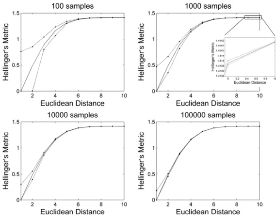
If the precision needed is not enough to generate disjoint intervals in competitive scenarios composed by multiple hypotheses, then the two-stage resampling can be repeated using a higher N1,
see Figure 6.
One can see in Figure 6 that the interval decreases with the increase of random samples, and that the exact value of nonparametric Hellinger’s metric, which is represented by a continuous line, is always contained in the estimated interval.
To verify the behavior of the resampling Estimator with the Parzen’s window 2 variation, we
studied the results for 0.1 to 2 with 0.1 increases, Figure 7. In all the cases, the exact value is within the estimated error bound. Hence, the error bound estimator proposed here leads to robust intervals estimation.
Figure 6. Illustration of an asymptotic study of the novel robust two-stage resampling interval estimator between the upper and lower interval limits for different number of random samples (a detailed view regarding the Euclidean distances between 9 and 10 was added to the 1,000 samples graphic so the behavior of the estimator can be easily confirmed.)
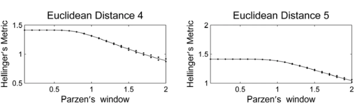
Figure 7. Illustration of the behavior of the new robust two-stage resampling interval estimator with the Parzen’s window variation from 0.1 to 2; the graphics regard Euclidean distances from 0 (zero) to 5; the upper and lower interval limits always contain the exact value that is represented by a continuous line.
Entropy 2013, 15 1621 Figure 7. Cont.
4. Conclusions
Hellinger’s metric was obtained from the generalized differential entropies and divergences. A nonparametric metric estimator based on Parzen’s window was introduced. We proposed a change of measure to allow a resampling method. With the change of measure proposed, it was possible to design a new two-stage resampling error bound estimator. The resampling error bound estimator also has the advantage of resampling just one density (the sum of normalized product densities) given by a nonparametric Parzen’s density with diagonal covariance, with asymptotic behavior. The new algorithm presented a robust behavior and very promising results. The asymptotic behavior allows to use this metric, in a competitive scenario with three or more densities, like clustering and image retrieval, to obtain disjoint intervals, simply by increasing the number of resampling samples. As to possible future work, two possible paths seem interesting: to evaluate Hellinger’s metric behavior on medical image processing and analysis as in [40,41], and to assess k-NN entropy estimation capability with the metric and heterocedastic data addressed here.
Acknowledgments
This paper is dedicated to André T. Puga, who initiated and supervised this work prior to his death. This work has been financially supported by Fundação para a Ciência e a Tecnologia (FCT), in Portugal, in the scope of the research project with reference PTDC/EEA-CRO/103320/2008.
Conflict of Interest
The authors declare no conflict of interest. References
1. Hellinger, E. Neue Begründung der Theorie quadratischer Formen von unendlichvielen Veränderlichen. Crelle 1909, 210–271.
2. Ali, S.M.; Silvey, S.D. A general class of coefficients of divergence of one distribution from another. J. R. Stat. Soc. Series B. 1966, 28, 131–142.
3. Ullah, A. Entropy, divergence and distance measures with econometric applications. J. Stat. Plan Inferace 1996, 49, 137–162.
4. Principe, J.C. Information Theoretic Learning Renyi's Entropy and Kernel Perspectives; Springer: New York, NY, USA, 2010.
5. Pardo, L. Statistical Inference Based on Divergence Measures; Chapman and Hall/CRC: Boca Raton, FL, USA, 2005; p. 483.
6. Kullback, S.; Leibler, R.A. On Information and Sufficiency. Ann. Math. Stat. 1951, 22, 79–86. 7. Bregman, L.M. The relaxation method of finding the common point of convex sets and its
application to the solution of problems in convex programming. USSR Comput. Math. Math. Phys. 1967, 7, 200–217.
8. Jeffreys, H. Fisher and inverse probability. Int. Stat. Rev. 1974, 42, 1–3.
9. Rao, C.R.; Nayak, T.K. Cross entropy, dissimilarity measures, and characterizations of quadratic entropy. IEEE Trans. Inf. Theory 1985, 31, 589–593.
10. Lin, J.H. Divergence measures based on the Shannon Entropy. IEEE Trans. Inf. Theory 1991, 37, 145–151.
11. Menéndez, M.L.; Morales, D.; Pardo, L.; Salicrú, M. (h, Φ)-entropy differential metric. Appl. Math. 1997, 42, 81–98.
12. Seth, S.; Principe, J.C. Compressed signal reconstruction using the correntropy induced metric. In Proceedings of IEEE International Conference on Acoustics, Speech and Signal Processing, Las Vegas, NV, USA, March 31–April 4, 2008; pp. 3845–3848.
13. Topsoe, F. Some inequalities for information divergence and Related measures of discrimination. IEEE Trans. Inf. Theory 2000, 46, 1602–1609.
14. Liese, F.; Vajda, I. On divergences and informations in statistics and information theory. IEEE Trans. Inf. Theory 2006, 52, 4394–4412.
15. Cubedo, M.; Oller, J.M. Hypothesis testing: A model selection approach. J. Stat. Plan. Inference 2002, 108, 3–21.
16. Puga, A.T.; Non-parametric Hellinger’s Metric. In Proceedings of CMNE/CILANCE 2007, Porto, Portugal, 13–15 June 2007.
17. Hartley, R.V.L. Transmission of information. Bell Syst. Tech. J. 1928, 7, 535–563.
18. Shannon, C.E. A mathematical theory of communication. Bell Syst. Tech. J. 1948, 27, 379–423. 19. Rényi, A. On Measures of Entropy and Information, Fourth Berkeley Symposium on Math.
Statist. and Prob; University of California: Berkeley: CA, USA, 1961; Volume 1, pp. 547–561. 20. Nonextensive Entropy: Interdisciplinary Applications; Gell-Mann, M.; Tsallis, C., Eds.; Oxford
University Press: New York, NY, USA, 2004.
21. Wolf, C. Two-state paramagnetism induced by Tsallis and Renyi statistics. Int. J. .Theor. Phys. 1998, 37, 2433–2438.
22. Gokcay, E.; Principe, J.C. Information theoretic clustering. IEEE Trans. Pattern Anal. Mach. Intell. 2002, 24, 158–171.
23. Ramshaw, J.D. Thermodynamic stability conditions for the Tsallis and Renyi entropies. Phys. Lett. A 1995, 198, 119–121.
24. Gibbs, A.L.; Su, F.E. On choosing and bounding probability metrics. Int. Stat. Rev. 2002, 70, 419–435.
25. Silverman, B.W. Density Estimation for Statistics and Data Analysis; Chapman and Hall: London, UK, 1986.
26. Scott, D.W. Multivariate Density Estimation: Theory, Practice, and Visualization; Wiley: New York, NY, USA, 1992.
Entropy 2013, 15 1623 27. Devroye, L. Non-Uniform Random Variate Generation; Springer-Verlag: New York, NY, USA, 1986. 28. Preda, V.C. The student distribution and the principle of maximum-entropy. Ann. Inst. Stat. Math.
1982, 34, 335–338.
29. Kapur, J.N. Maximum-Entropy Models in Science and Engineering; Wiley: New York, NY, USA, 1989. 30. The Probable Error of a Mean. Available online: http://www.jstor.org/discover/10.2307/2331554?
uid=2&uid=4&sid=21102107492741/ (accessed on 28 April 2013).
31. Leonenko, N.; Pronzato, L.; Savani, V. A class of Renyi information estimators for multidimensional densities. Ann. Stat. 2008, 36, 2153–2182.
32. Li, S.; Mnatsakanov, R.M.; Andrew, M.E. k-nearest neighbor based consistent entropy estimation for hyperspherical distributions. Entropy 2011, 13, 650–667.
33. Penrose, M.D.; Yukich, J.E. Laws of large numbers and nearest neighbor distances. In Advances in Directional and Linear Statistics; Wells, M.T., SenGupta, A., Eds.; Physica-Verlag: Heidelberg, Germany, 2011; pp. 189–199.
34. Misra, N.; Singh, H.; Hnizdo, V. Nearest neighbor estimates of entropy for multivariate circular distributions. Entropy 2010, 12, 1125–1144.
35. Mnatsakanov, R.; Misra, N.; Li, S.; Harner, E. k-Nearest neighbor estimators of entropy. Math. Method. Stat. 2008, 17, 261–277.
36. Wang, Q.; Kulkarni, S.R.; Verdu, S. Divergence estimation for multidimensional densities via k-nearest-neighbor distances. IEEE Trans. Inf. Theory 2009, 55, 2392–2405.
37. Hall, P.; Park, B.U.; Samworth, R.J. Choice of neighbor order in nearest-neighbor classification. Ann. Stat. 2008, 36, 2135–2152.
38. Nigsch, F.; Bender, A.; van Buuren, B.; Tissen, J.; Nigsch, E.; Mitchell, J.B.O. Melting point prediction employing k-nearest neighbor algorithms and genetic parameter optimization. J. Chem. Inf. Model. 2006, 46, 2412–2422.
39. Beyer, K.; Goldstein, J.; Ramakrishnan, R.; Shaft, U. When Is “Nearest Neighbor” Meaningful? In Proceedings of 7the International Conference on Database Theory, Jerusalem, Israel, 10–12 January 1999; pp. 217–235.
40. Vemuri, B.C.; Liu, M.; Amari, S.I.; Nielsen, F. Total bregman divergence and its applications to DTI analysis. IEEE Trans. Med. Imag. 2011, 30, 475–483.
41. Liu, M.; Vemuri, B.; Amari, S. I.; Nielsen, F. Shape retrieval using hierarchical total bregman soft clustering. IEEE T. Pattern Anal. 2012, 34, 2407–2419.
© 2013 by the authors; licensee MDPI, Basel, Switzerland. This article is an open access article distributed under the terms and conditions of the Creative Commons Attribution license (http://creativecommons.org/licenses/by/3.0/).