Reliability Function Estimator with Exponential Failure Model for Engineering Data

(1)

Abstract This paper provides estimation of reliability of a component subjected to life testing and the procedure includes essentially polling of two samples of failure data, where the component follows exponential failure model. We assumed that some prior information is available in the form of an initial

guess value (

θ

_o) about the value of the parameter (

θ

) of exponential distribution from the past, and proposed a two stage shrinkage pooling estimator (TSPE) of reliability function of exponential distribution using complete failure data. The expressions for the bias, mean squared error, expected sample size and relative efficiency are derived. Conclusions regarding the constants involved in the proposed estimator are presented. Simulation, comparisons, and numerical results are reported. The proposed estimator fairs better than the classical two stage pooling estimator.

Index Terms exponential failure model, reliability function, relative efficiency, two stage shrunken.

I. INTRODUCTION

The goal of system modeling is to provide quantitative forecasts of various system performance measures such as downtime, availability, number of failures, capacity, and cost. Evaluation of these measures is important to make optimal decisions when designing a system to either minimize overall cost or maximize a system performance measure within the allowable budget and other performance-based constraints.

In general, the shape or type of failure distribution depends upon the component's failure mechanisms. Similarly, the shape or type of repair distribution depends upon several factors associated with component repairs. Several methods are used to determine the distribution that best fits a given failure or repair pattern. Or, if failures or repairs are known to follow a particular distribution, the specific parameters that define this pattern can be determined by using the known failure and repair times.

As noted earlier, determining the failure and repair distributions of your system and its components is a significant part of evaluating the reliability of your design. If the failure rate is constant, which is generally true for electronic components during the main portion of their useful life, the reliability of the component follows an exponential distribution with p.d.f.

Manuscript received February 9, 2009. This work was supported in part by the University of Nizwa.

Zuhair A. Al-Hemyari is a professor with the Department of mathematical and Physical Sciences, College of Arts and Sciences, University of Nizwa, P.O. Box 33, PC616, Nizwa, Oman, on leave from the Department of Mathematics, College of Ibn Al-Haithm, Baghdad University, Baghdad, Iraq. (e-mails: alhemyari@unizwa.edu.om ; drzuhair111@yahoo.com ).

.

0 ,

0 ;

))

(exp(

)

|

(

x

θ

=

θ

−

x

θ

x

>

θ

>

f

(1)

In the context of reliability evaluation and life testing, a number of engineering data have been examined (see [5] and [14]) and it was shown that the exponential distribution give quite a good fit for most cases. Furthermore, the exponential distribution is a very commonly used distribution in reliability engineering and has a wide range of applications in analyzing the reliability and availability of electronic systems, various queuing networks, and Markov chains; whereas the reliability of a given system (or component) for a given time has been defined as the probability that the system (or component) has a length of life greater than t, i.e.,

.

0 0,

t

,

)

(-t

exp

)

(

)

(

>

=

>

=

θ

t

x

P

t

R

(2)

The classical estimator

θ

ˆ

of

θ

and hence of

R

(

t

)

can easily be obtained without any complicated mathematicalaid. The problem of estimation of

θ

and

R

(

t

)

was considered by several authors (see [5] and [14]).

2. INCORPORATING A GUESS VALUE

θ

_o

,

AND TSPE In many practical circumstances, physical experts have some prior information regarding the value of

θ

due to past experiences, and apply it latently to inference of the actual model. However, in certain situations the prior information is available only in the form of an initial guess value (natural origin)

θ

_o of

θ

. For example, a bulb producer may know that the average life time of his product may be close to 1000 hours. Here we may take

θ

_o

=

1000

.

In such a situation it is

natural to start with an estimator

θ

ˆ

(e.g. MLE) of

θ

and modify it by moving it closer to

θ

_o, so that the resulting

estimator, though perhaps biased, has smaller mean squared

error than that of

θ

ˆ

in some interval around

θ

_o . This

method of constructing an estimator of

θ

that incorporates the prior information

θ

_o leads to what is known as a

shrunken estimator.

A standard problem in life testing deals with estimation of the parameter

θ

and

R

(

t

)

on the basis of less time and minimum cost of experimentation. The cost of experimentation can be achieved by using any prior information available about

θ

and devising a two stage shrunken pooling estimator (TSPE) in which it is possible to

Reliability Function Estimator with Exponential

Failure Model for Engineering Data

(2)

obtain an estimator from a small first stage sample and an additional second stage sample is required only if this estimator is not reliable. A TSPE of

θ

is defined as follows:

let

X

₁_i

,

i

=

1 ,

2 ,

...

,

n

₁ be a random sample of size

,

1

n

<

where the variables are distributed with p.d.f. (1) and

θ

ˆ

₁ be a good estimator of

θ

based on

n

₁ observations. Construct a region

R

in the space of

θ

_,

based on the prior

value O

θ

and an appropriate criterion. If

θ

ˆ

₁

∈

R

,

use the estimator

k

(

θ

ˆ

₁

−

θ

_o

)

+

θ

_o

,

for

θ

where

0 ≤

k

≤

1 .

But if

θ

ˆ

₁

∉

R

, obtain

X

₂_i

,

i

=

1 ,

2 ,

...

,

n

₂

,

n

₂

=

n

−

n

₁

,compute

θ

ˆ

₂ , and then pool

θ

ˆ

₁ and

θ

ˆ

₂ to find

.

/

)

ˆ

(

ˆ

2 2 1

1

n

θ

=

+

The TSPE of

θ

is thus given by

}

{

[

(

ˆ

)

]

ˆ

,

~

1 o o

I

R

I

_R

k

θ

=

−

+

(3) where

I

_R and

I

_Rare respectively the indicator functions of

the acceptance region

R

and the rejection region

R

. It may be noted here that TSPE of the parameter

θ

for complete, type

I

and type

II

censored data has also been considered by several authors (see [1]-[4], [6]-[9], [12] and [13]). In this paper we consider the problem of estimation of the reliability function

R

(

t

)

in the exponential distribution when the information regarding

θ

is available in the form of initial guess value

θ

_O

.

The general case of TSPE of

R

(

t

)

has been proposed and studied. The expressions for the bias, mean squared error, expected sample size and relative efficiency are obtained. Some numerical results and conclusions drawn therefrom are presented.

3. ESTIMATOR ASSUMPTIONS AND DERIVATION

As mentioned, the exponential distribution serves as a very useful model in analyzing the life testing and reliability data. Among the different type of data, interestingly, the complete and censored data (type I and type II) have received a considerable attention particularly in the reliability analysis. In this section first we define the general proposed estimator based on complete failure data, then we describe a choice of the region

R

, and finally we obtain the necessary expressions of the proposed estimator.

3.1 FAILURE DATA

Suppose

n

_j

,

i

=

1 ,

2

items are subjected to life test and the test is terminated after all items have failed. Let

nj j

j

X

₁

,

₂

,

...

,

be the random failure times of size

j

n

and suppose the failure times are exponentially

distributed with p.d.f. (1). The MLE

θ

ˆ

_j of

θ

based on the

above items is given by

,

2 ,

1 /

1 ˆ

₌

_X

_j

₌

j

θ

(4)

where

2 r

_j

θ

/

θ

ˆ

_j distributed as chi square random variable with 2rj degrees of freedom (see [10]). The proposed TSPE

of

R

(

t

)

in this case is definedby:

(

)

[

]

(

)

[

]

_⎪⎭

⎪

⎬

⎫

⎪⎩

⎪

⎨

⎧

+

−

+

−

=

R R o o

I

n

t

I

k

t

R

/

))

ˆ

(

)

ˆ

(

exp(

)

ˆ

(

exp(

)

(

~

2 2 1 1 1

θ

(5)

3.2 CHOICE FOR REGION

R

Estimator (5) is completely obtained by specifying the region R. A choice for the region

R

is considered here. In this choice we follow Katti’s (see [10]) approach. That is, let

R

be the region which minimizes

MSE

(

θ

~

|

θ

_o

,

R

)

(see (3)). This gives

{

}

[

.(

0 ,

(

1 )),

(

1 )

]

,

0 )

|

ˆ

(

)

ˆ

)(

|

ˆ

(

2 )

ˆ

)(

(

:

ˆ

0 0 0 1 2 2 1 0 1 0 1 2 2 1 2 0 1 2 2 1 2 1

v

Max

MSE

n

xB

x

n

k

R

+

−

=

≤

−

=

θ

(6) where , / ), 2 )( ( ) ( , 2 ) 1 )( /( ) ( 2 1 2 2 1 2 2 2 2 2 2 1 2 2 2 1 2 2 1 n n k n n n k n n n n p n n n k n n n p v > − + − + = − − − + =

and

n

₂

>

2 .

3.3 EXPRESSIONS

Let

R

=

[

a

_j

,

b

_j

]

The expressions for the bias, bias ratio, expected sample size, and relative efficiency of

R

~

(

t

)

are obtained as follows:

,

1 ))

)

/(

2 (

)

))

/(

2 (

))

/(

(

2 (

))

/(

(

)

/

4 ((

))

/(

(

)

2 (

)

(

2 /

))

(

)

(

~

(

)

|

)

(

~

(

2 1 2 1 2 1 2 1 2 1 2 2 2 / 2 1 2 2 2 1 2 / 2 1 2 1 1 2 / 1 ) 1 ) 1 (( ( 1 1 2 2 1 1 1

−

+

−

+

Γ

+

=

−

=

− − − −

n

t

n

t

n

t

n

x

n

t

n

x

n

e

n

t

n

k

t

n

k

t

n

e

t

R

t

R

E

R

t

R

B

n n n r t r n r k t t

θ

β

θ

β

θ

β

θ

β

θ

θ λ θ θ (7)

(3)

{

[

]

[

]

1 }

,

))

/(

(

2 (

))

/(

(

2 (

)

/(

2 (

2 ))

)

/(

2 (

)

))

/(

2 (

)

8 (

)

))

/(

2 (

2 ))

(

)

(

/

1 (

))

/(

(

))

/(

(

4 )

2 (

)

(

4 )

2

2 (

)

2 )))(

(

/

1 (

2 (

)

|

)

(

~

(

2 1 2 1 2 1 2 1 2 1 2 2 2 1 2 1 2 1 2 1 2 1 2 2 2 / ) ( 2 1 2 / 2 1 2 2 2 / 2 1 2 1 1 2 / 1 )) 1 ) 1 ( ( 1 2 / 1 1 ) 1 ) 1 (( 2 1 1 2 1 1 2 2 1 2 1 1 1 1

+

−

+

−

+

−

+

Γ

+

−

Γ

=

+ − − − − − − −

n

t

n

t

n

x

n

t

n

t

n

t

n

x

n

t

n

e

x

n

t

n

x

n

t

n

e

k

t

n

k

t

n

e

k

t

n

k

t

n

x

e

R

t

R

MSE

n n n n n n t n n n n t n n k t n r k t t

θ

β

θ

β

θ

β

θ

β

θ

β

θ

β

θ

β

θ

β

θ

θ θ λ θ λ θ θ

where

β

_p₋₁

(

2 ab

)

(see[14]) is the Bessel function of order

,...,.,

2 ,

1 (.),

(.)

,

2 ,

1 ,

p

=

r

+

j

=

₋

p

=

p

_j

β

_p

β

_p

given by

),

1 (

)

1 (

2 /

)

1 (

)

/

(

2 )

2 (

)

/

(

2

1 2 0 2 / ) 1 ( 1 2 / ) 1 ( ) / ( 0

+

Γ

+

Γ

−

=

+ + ∞ = − − − + − − ∞

∑

∫

p

n

p

xt

x

b

a

ab

x

b

a

dX

e

X

n p n p p p p p X b aX p

β

(9)

and

β

_p₋₁

(

2 ab

)

, is an incomplete Bessel’s function, where the integration (summation) is over the interval

.

/

2 ,

/

2 ,

],

,

[

* * * * * * * j j j j j j j j j j

b

n

b

a

n

a

b

a

b

a

R

θ

=

<

=

The efficiency of

R

~

2

(

t

)

relative to

R

ˆ

(

t

)

is given by:

),

|

)

(

~

(

/

))

(

ˆ

(

))

(

ˆ

|

)

(

~

(

R

t

R

t

MSE

R

t

MSE

R

t

R

RE

=

(10)

where

{

[

] }

1 .

)

/(

2 (

))

)

/(

(

2 (

2 )

))

/(

2 (

)

))

/(

2 (

2

2 ))

(

)

(

/

1 (

))

/(

(

))

/(

(

4 (

))

(

ˆ

(

2 1 2 2 2 1 2 1 2 1 2 1 2 1 2 2 2 / 2 / 2 1 2 / 2 1 2 2 2 / 2 1 2 1 2 2 1 1 2 2 1 2 1

+

−

+

Γ

+

=

−

n

t

n

x

n

t

n

t

n

x

n

t

n

e

x

n

t

n

x

n

t

n

e

t

R

MSE

n n n n t n n n n t t

θ

β

θ

β

θ

β

θ

β

θ

θ θ θ (11)

The expected sample size required to obtain

R

~

(

t

)

is given by

)),

,

2 (

)

,

2 (

(

)

),

(

~

|

(

n

R

t

R

n

₂

G

n

₁

b

G

n

₁

a

E

=

−

(12)

where

G

(

2 n

₁

,.)

is the cumulative distribution function of a chi-square random variable with

2 n

₁degrees of freedom.

4. SIMULATION AND NUMERICAL RESULTS

For the testimator

R

~

(

t

)

, the relative efficiency, bias ratio, expected sample size and percentage of the overall sample

size saved

100 (

n

₂

/

n

)

x

Pr(

θ

ˆ

₁

∈

R

)

were computed for

)

(

~

t

R

by taking

,

3 )

3 .

0 (

3 .

0 ,

12 )

2 (

2 ,

12 )

2 (

4

₂

1

=

n

=

t

θ

=

n

and

))

/

(

10

1 .

0 ≤

λ

≤

λ

=

θ

₀

θ

. The Katti’s type region

R

(as in (6)) is defined for

k

>

n

₁

/

n

₂

.

Relative

efficiency of

R

~

(

t

)

is computed

for

k

=

(

n

₁

/

n

₂

,

)

+

10

−i,

i

=

1 (

1 )

10 ,

and it has been observed that the relative efficiency is high for

i

=

7 ,

therefore, when using the region

R

the value

7 2

1

/

)

10 (

+

−

=

n

k

is recommended. Some of these

results are presented in tables 1 to 4. The following observations are drawn on the basis of these computations.

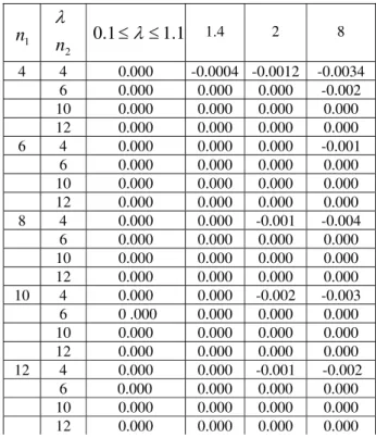
1. The testimator

R

~

(

t

)

is biased. The bias ratio is approximately zero (to the third decimal point) of

R

~

(

t

)

for

,

1

1 .

0 ≤

λ

≤

n

₁,

n

₂, and

t

θ

, and increasing very slowly with increases of

λ

. In Table 1 we have presented some sample values of the bias ratio.

2. The testimator

R

~

(

t

)

for

0 .

1 ≤

λ

≤

10 ,

has smaller mean squared error than the pooled estimator

R

ˆ

(

t

)

(see Table 2).

3. Relative efficiency of

R

~

(

t

)

is a concave function of

λ

, i.e., the proposed testimators have maximum efficiency in the neighborhood of

λ

≅

1 .

4

.Some of these computations are given in Table 2.

(4)

4. Efficiency of

R

~

(

t

)

relatively to the classical estimator

)

(

ˆ

_t

R

is a decreasing function of

t

θ

,

n

₂

,

and

n

₁. i.e.,

,

3 .

0 ,

4 ,

4

₂

1

≅

n

≅

t

θ

=

n

and gives higher relative

efficiency than for other values of

t

θ

,

n

₂

,

and

n

₁

(Table2).

5.

E

(

n

|

R

~

(

t

))

is generally smaller than

n

when

λ

≅

1 .

4

and increases very slowly with decreases or increases of

λ

(also see Table 3).

6. The percentage of the overall sample saved of

R

~

(

t

)

is maximum when

θ

_O is close to

θ

,

the percentage is about

(5%-15%) for small values of

n

₁

.

i.e.,

,

12 )

2 (

2 ,

4

₂

1

≅

n

≅

n

0 .

5 ≤

λ

≤

1 .

7 ,

and gives smaller

percentage than for other values of

λ

,

n

₂

,

and

n

₁ (see Table 4).

ACKNOWLEDGMENTS

The author is thankful to the conference committee and to the referees, whose suggestions improved the paper considerably.

REFERENCES

[1] S. R. Adke, V.B. Waikar, and F.J. Schuurmann, “A two stage shrinkage testimator for the mean of an exponential distribution,” Commun. Statist. Theor. Meth., vol.16, 1987, pp.1821-1834.

[2] Z. A. Al-Hemyari, “On Stein type two-stage shrinkage testimator (Accepted for Publication),” International J. of Modeling and Simulation, to be published.

[3] Z. A. Al-Hemyari, “Life testing and reliability analysis with exponential failure model,” International J. of Modeling and Simulation, submitted for publication. [4] Z. A. Al-Hemyari, A. Kurshid and A. Al-Gebori“On Thompson testimator for the mean of normal distribution.”. REVISTA INVESTIGACION OPERACIONL vol.30, P109 116,2009.

[5] B.V. Gnedenko, Ku. K. Balyayev, and A. D. Solovyev, Mathematical Methods of Reliability Theory. Academic Press, 1969.

[6] D.V. Gokhale, and S.R. Adke, “ On two stage shrinkage testimation for exponential distribution,” Commun. Statist. Theory Meth., vol.18, 1989, pp. 3203-3213. [7] B.R. Handa, N.S. Kambo, and Z.A. Al-Hemyari, “ On double stage shrunken estimator for the mean of exponential distribution,” IAPQR Transactions, vol.13, 1988, pp.19-33.

[8] N.S. Kambo, B.R. Handa, and Z. A. Al-Hemyari, “ Double stage shrunken estimator for the exponential mean life in censored samples,” International Journal of Management and Systems, vol.7, 1991, pp.283-301. [9] N.S. Kambo, B.R. Handa, and Z.A. Al-Hemyari, “ On shrunken estimators for exponential scale parameter,” J. of Statistical Planning and Inferences, vol.24, 1990 pp.87-94.

[10] S.K. Katti, (1962). “Use of some a prior knowledge in the estimation of means from double samples, “ Biometrics, vol.,18,139-147. [11] S.K. Sinha, Reliability and Life Testing. Wiley Eastern Limited, 1986.

Table 1: Showing

B

(

R

~

(

t

)

|

R

)

when

t

θ

=

0 .

3

and different values of

n

₁,

n

₂ and

λ

.

[12] U. Singh,. and Kumar, A, “Shrinkage estimators for exponential scale parameter using multiply type II censoring,” Austrian J. of Statist, vol.34, 2005, pp.39-49.

[13] R. Srivastava and V. Tanna , “Double stage shrinkage testimator of the scale parameter of an exponential life model under general entropy loss function” Commun. Statist. Theor. Meth.,

vol.36, 2007, pp.283-295.

[14] G. N. Watson, Treatise on the Theory of Bessel Function, Cambridge University Press, 1952.

1

n

2

n

λ

1 .

1

1 .

0 ≤

λ

≤

1.4 2 8

4 4 0.000 -0.0004 -0.0012 -0.0034

6 0.000 0.000 0.000 -0.002

10 0.000 0.000 0.000 0.000

12 0.000 0.000 0.000 0.000

6 4 0.000 0.000 0.000 -0.001

6 0.000 0.000 0.000 0.000

10 0.000 0.000 0.000 0.000

12 0.000 0.000 0.000 0.000

8 4 0.000 0.000 -0.001 -0.004

6 0.000 0.000 0.000 0.000

10 0.000 0.000 0.000 0.000

12 0.000 0.000 0.000 0.000

10 4 0.000 0.000 -0.002 -0.003

6 0 .000 0.000 0.000 0.000

10 0.000 0.000 0.000 0.000

12 0.000 0.000 0.000 0.000

12 4 0.000 0.000 -0.001 -0.002

6 0.000 0.000 0.000 0.000

10 0.000 0.000 0.000 0.000

12 0.000 0.000 0.000 0.000

(5)

Table 2: Showing

RE

(

R

~

(

t

)

|

R

ˆ

(

t

))

when

t

θ

=

0 .

3 n

1,

n

2 and

λ

.

1

n

2

n

λ

0.1 0.4 0.5 0.6 0.7 0.8 0.9 1.0 1.1 1.4 2 8

4 4 1.00 1.05 1.41 1.82 2.08 2.46 2.85 3.47 3.47 5.94 2.12 1.03

6 1.00 1.05 1.28 1.35 2.18 2.51 2.77 3.15 3.31 5.68 2.09 1.03

10 1.00 1.07 1.19 1.69 2.08 2.31 2.75 2.33 2.78 5.58 2.08 1.03

12 1.00 1.16 1.38 1.69 1.91 1.82 2.27 3.21 2.75 5.58 2.08 1.03

6 4 1.00 1.08 1.23 1.33 1.48 1.74 2.07 2.12 2.12 5.58 2.08 1.03

6 1.00 1.03 1.23 1.44 1.49 1.72 2.17 2.22 2.24 5.20 1.92 1.01

10 1.00 1.02 1.11 1.34 1.69 1.69 2.32 2.45 2.46 4.96 1.89 1.01

12 1.00 1.03 1.11 1.27 1.49 1.76 2.02 2.25 2.29 4.96 1.89 1.01

8 4 1.00 1.04 1.07 1.27 1.41 1.42 1.56 1.54 1.54 4.96 1.89 1.01

6 1.00 1.03 1.12 1.26 1.41 1.46 1.65 1.65 1.69 4.96 1.89 1.01

10 1.00 1.02 1.12 1.26 1.49 1.51 1.81 1.01 1.71 4.90 1.74 1.00

12 1.00 1.02 1.12 1.27 1.33 1.53 1.91 1.91 1.99 4.88 1.74 1.00

10 4 1.00 1.01 1.07 1.10 1.18 1.28 1.29 1.30 1.31 4.88 1.74 1.00

6 1.00 1.00 1.06 1.15 1.25 1.28 1.33 1.37 1.38 4.88 1.74 1.00

10 1.00 1.00 1.03 1.10 1.23 1.44 1.49 1.50 1.53 3.56 1.60 1.00

12 1.00 1.00 1.07 1.10 1.23 1.38 1.48 1.51 1.53 3.50 1.60 1.00

12 4 1.00 1.00 1.04 1.06 1.13 1.15 1.16 1.17 1.17 3.50 1.59 1.00

6 1.00 1.00 1.02 1.09 1.12 1.19 1.21 1.21 1.28 3.50 1.59 1.00

10 1.00 1.00 1.03 1.07 1.14 1.27 1.31 1.31 1.34 3.50 1.59 1.00

12 1.00 1.00 1.02 1.11 1.16 1.31 1.35 1.35 1.37 3.37 1.59 1.00

(6)

Table 3: Showing

E

(

n

|

R

~

(

t

),

R

)

when

t

θ

=

0 .

3 n

₁,

n

₂ and

λ

.

1

n

2

n

λ

0.1 0.4 0.5 0.6 0.7 0.8 0.9 1.0 1.1 _1.4 ₂ ₈

4 4 8.00 7.93 7.85 7.74 7.63 7.54 7.46 7.39 7. 36 7.23 7.44 7.56

6 10.00 9.91 9.79 9.64 9.49 9.36 7.25 9.17 9.11 9.00 9.20 9.52

10 14.00 13.86 11.68 13.44 13.20 12.98 12.81 12.69 12.61 12.43 12.61 12.62 12 16.00 15.85 15.84 15.62 15.34 15.05 14.79 14.44 14.35 14.10 14.39 14.41

6 4 10.00 9.98 9.93 9.86 9.78 9.71 9.46 9.59 9.57 9.32 9.52 9.61 6 12.00 11.97 11.91 11.81 11.71 11.59 11.51 11.44 11.41 11.22 11.42 11.54

10 16.00 15.96 15.87 15.71 15.53 15.35 15.21 15.12 15.07 14.93 14.65 14.76 12 18.00 17.99 17.84 17.66 17.46 17.23 17.08 16.96 16.90 16.71 16.93 17.11

8 4 12.00 11.99 11.96 11.92 11.86 11.79 11.73 11.69 11.67 11.34 11.57 11.63

6 14.00 13.99 13.97 13.91 13.86 13.79 13.74 13.69 13.67 13.43 13.65 13.77 10 18.00 17.99 17.94 17.83 17.69 17.55 17.42 17.34 17.17 16.99 17.12 17.25

12 20.00 19.98 19.92 19.80 19.63 19.46 19.32 19.22 19.17 19.02 19.25 19.36

10 4 14.00 13.99 13.89 13.95 13.89 13.84 13.79 13.76 13.74 13.85 13.91 13.99

6 16.00 15.99 15.98 15.93 15.86 15.78 15.71 15.67 15.64 15.63 15.75 15.86

10 20.00 19.99 19.97 19.89 19.78 19.86 19.55 19.47 19.45 19.23 19.45 19.56 12 22.00 21.99 21.96 21.88 21.74 21.59 21.46 21.38 21.35 21.21 21.46 21.58

12 4 16.00 15.99 15.99 15.96 15.92 15.87 15.83 15.79 15.78 15.52 15.72 15.84

6 18.00 17.99 17.99 17.95 17.89 17.82 17.76 17.76 17.72 17.61 17.82 17.89

(7)

Table 4: Showing

100 (

n

₂

/

n

)

x

Pr(

θ

ˆ

₁

∈

R

)

when

t

θ

=

0 .

3 n

₁

,

n

₂

,

and

λ

.

1

n

2

n

λ

0.1 0.4 0.5 0.6 0.7 0.8 0.9 1.0 1.1 _1.4 ₂ ₈

4 4 0.01 4.14 6.33 8.01 9.14 9.81 10.11 10.11 9.90 9.72 9.60 6.10

6 0.01 4.97 7.59 9.61 10.97 11.77 12.13 12.14 11.88 11.77 11.65 7.12

10 0.01 5.92 9.04 11.44 13.06 14.01 14.44 14.45 14.15 14.00 13.88 8.31

12 0.01 6.21 9.49 12.01 13.71 14.71 15.16 15.17 14.86 14.70 14.58 9.01

6 4 0.00 0.54 1.21 2.11 3.08 3.95 4.36 5.12 5.43 5.26 5.15 1.22

6 0.00 0.68 1.51 2.64 3.85 4.64 5.79 6.40 6.79 6.39 6.28 1.55

10 0.00 0.85 1.89 3.30 4.82 6.17 7.24 8.00 8.49 8.20 8.14 1.93

12 0.00 0.91 2.02 3.52 5.14 6.58 7.72 8.53 9.05 8.82 8.70 2.32

8 4 0.00 0.10 0.30 0.61 1.05 1.59 2.14 2.63 3.02 2.84 2.73 1.00

6 0.00 0.13 0.38 0.78 1.35 2.04 2.75 3.38 3.88 3.55 3.44 1.31

10 0.00 0.17 0.49 1.01 1.75 2.65 3.56 4.38 5.03 4.65 4.55 1.52

12 0.00 0.18 0.53 1.09 1.89 2.86 3.85 4.73 5.43 5.21 5.16 1.71

10 4 0.00 0.02 0.09 0.22 0.41 0.68 1.02 1.39 1.74 1.43 1.31 0.34

6 0.00 0.02 0.12 0.28 0.54 0.90 1.34 1.82 2.28 2.00 1.93 0.52

10 0.00 0.03 0.15 0.38 0.72 1.20 1.79 2.43 3.04 2.78 2.65 0.61

12 0.00 0.03 0.17 0.41 0.78 1.30 1.95 2.65 3.31 3.08 2.99 0.70

12 4 0.00 0.00 0.03 0.09 0.19 0.33 0.52 0.77 1.03 0.88 0.76 0.16

6 0.00 0.00 0.03 0.12 0.25 0.44 0.70 1.02 1.38 1.09 0.89 0.22

10 0.000 0.01 0.05 0.16 0.34 0.60 0.95 1.40 1.88 1.53 1.41 0.30

12 0.000 0.01 0.05 0.18 0.37 0.66 1.05 1.54 2.06 1.77 1.65 0.31