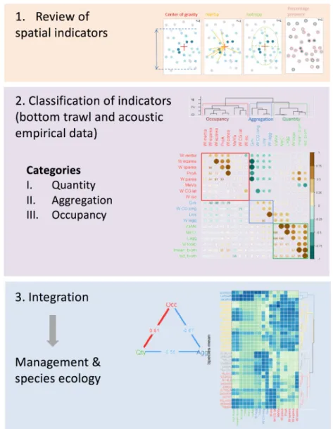
Integrating spatial indicators in the surveillance of exploited marine ecosystems
21
0
0
Texto
Imagem

+4
Documentos relacionados