Revisit of Logistic Regression:
Efficient Optimization and Kernel Extensions
Takumi Kobayashi
National Institute of Advanced Industrial Science and Technology Umezono 1-1-1, Tsukuba, 305-8568, Japan
Email: [email protected]
Kenji Watanabe
Wakayama University
Sakaedani 930, Wakayama, 640-8510, Japan Email: [email protected]
Nobuyuki Otsu
National Institute of Advanced Industrial Science and Technology Umezono 1-1-1, Tsukuba, 305-8568, Japan
Email: [email protected]
Abstract—Logistic regression (LR) is widely applied as a powerful classification method in various fields, and a variety of optimization methods have been developed. To cope with large-scale problems, an efficient optimization method for LR is required in terms of computational cost and memory usage. In this paper, we propose an efficient optimization method using non-linear conjugate gradient (CG) descent. In each CG iteration, the proposed method employs the optimized step size without exhaustive line search, which significantly reduces the number of iterations, making the whole optimization process fast. In addition, on the basis of such CG-based optimization scheme, a novel optimization method for kernel logistic regression (KLR) is proposed. Unlike the ordinary KLR methods, the proposed method optimizes the kernel-based classifier, which is naturally formulated as the linear combination of sample kernel functions, directly in the reproducing kernel Hilbert space (RKHS), not the linear coefficients. Subsequently, we also propose the multiple-kernel logistic regression (MKLR) along with the optimization of KLR. The MKLR effectively combines the multiple types of kernels with optimizing the weights for the kernels in the framework of the logistic regression. These proposed methods are all based on CG-based optimization and matrix-matrix computation which is easily parallelized such as by using multi-thread programming. In the experimental results on multi-class classifications using various datasets, the proposed methods exhibit favorable performances in terms of classification accuracies and computation times.
I. INTRODUCTION
A classification problem is an intensive research topic in the pattern recognition field. Especially, classifying the feature vectors extracted from input data plays an important role; e.g., for image (object) recognition [1] and detection [2], motion recognition [3], natural language processing [4]. Nowadays, we can collect a large amount of data such as via internet, and thus large-scale problems have being frequently addressed in those fields to improve classification performances.
In the last decade, the classification problems have been often addressed in the large margin framework [5] as rep-resented by support vector machine (SVM) [6]. While those methods are basically formulated for linear classification, they are also extended to kernel-based methods by employing kernel functions and produce promising performances. However, they are mainly intended for binary (two) class problems and it
is generally difficult to extend the method toward the multi-class problems without heuristics such as a one-versus-rest approach. Several methods, however, are proposed to cope with the multi-class problems, e.g., in [7]. Another drawback is that the optimization in those methods has difficulty in parallelization. The SVM-based methods are formulated in quadratic programming (QP). Some successful optimization methods to solve the QP, such as sequential minimal opti-mization (SMO) [8], are based on a sequential optiopti-mization approach which can not be easily parallelized. Parallel com-puting currently developed such as by using GPGPU would be a key tool to effectively treat large-scale data.
On the other hand, logistic regression has also been suc-cessfully applied in various classification tasks. Apart from the margin-based criterion for the classifiers, the logistic regression is formulated in the probabilistic framework. Therefore, it is advantageous in that 1) the classifier outputs (class) posterior probabilities and 2) the method is naturally generalized to the multi-class classifiers by employing a multi-nominal logistic function which takes into account the correlations among classes. While the optimization problem, i.e., objective cost function, for logistic regression is well-defined, there is still room to argue about its optimization method in terms of computational cost and memory usage, especially to cope with
large-scale problems. A popular method,iterative reweighted
least squares, is based on the Newton-Raphson method [9] requiring significant computation cost due to the Hessian.
In this paper, we propose an efficient optimization method for the logistic regression. The proposed method is based on non-linear conjugate gradient (CG) descent [10] which is directly applied to minimize the objective cost. The non-linear CG is widely applied to unconstrained optimization problems, though requiring an exhaustive line search to determine a step size in each iteration. In the proposed method, we employ the optimum step size without the line search, which makes the whole optimization process more efficient by significantly reducing the number of iterations. In addition, we propose a novel optimization method for kernel logistic regression (KLR) on the basis of the CG-based optimization scheme. Unlike the ordinary KLR methods, the proposed method optimizes the kernel-based classifier, which is naturally formulated as the linear combination of sample kernel functions as in SVM,
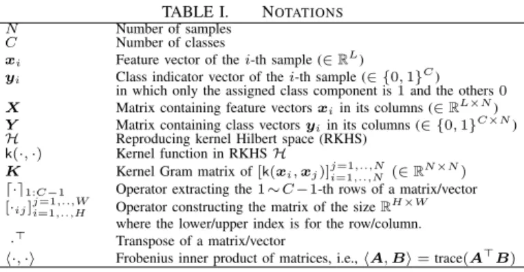
TABLE I. NOTATIONS
N Number of samples
C Number of classes
xi Feature vector of thei-th sample (∈RL)
yi Class indicator vector of thei-th sample (∈ {0,1}C) in which only the assigned class component is1and the others0 X Matrix containing feature vectorsxiin its columns (∈RL×N) Y Matrix containing class vectorsyiin its columns (∈ {0,1}C×N)
H Reproducing kernel Hilbert space (RKHS)
k(·,·) Kernel function in RKHSH
K Kernel Gram matrix of[k(xi,xj)]j=1,..,N
i=1,..,N (∈R N×N)
⌈·⌉1:C−1 Operator extracting the1∼C−1-th rows of a matrix/vector
[·ij]ji=1=1,..,H,..,W Operator constructing the matrix of the sizeR H×W where the lower/upper index is for the row/column.
·⊤
Transpose of a matrix/vector
·,· Frobenius inner product of matrices, i.e.,A,B=trace(A⊤
B)
rectly in the reproducing kernel Hilbert space (RKHS), not the linear coefficients of samples. Subsequently, multiple-kernel logistic regression (MKLR) is also proposed as multiple-kernel learning (MKL). The MKL combines the multiple types of kernels with optimizing the weights for the kernels, and it has been addressed mainly in the large margin framework [11]. The proposed MKLR is formulated as a convex form in the framework of logistic regression. In the proposed formulation, by resorting to the optimization method in the KLR, we optimize the kernel-based classifier in sum of multiple RKHSs and consequently the linear weights for the multiple kernels. In summary, the contributions of this paper are as follows;
• Non-linear CG in combination with the optimum step size
for optimizing logistic regression.
• Novel method for kernel logistic regression to directly
optimize the classifier in RKHS.
• Novel method of multiple-kernel logistic regression.
Note that all the proposed methods are based on the CG-based optimization and the computation cost is dominated by matrix-matrix computation which is easily parallelized.
The rest of this paper is organized as follows: the next section briefly reviews the related works of optimization for logistic regression. In Section III, we describe the details of the proposed method using non-linear CG. And then in Section IV and Section V we propose the novel optimization methods for kernel logistic regression and for multiple-kernel logistic regression. In Section VI, we mention the parallel computing in the proposed methods. The experimental results on various types of multi-class classification are shown in Section VII. Finally, Section VIII contains our concluding remarks.
This paper contains substantial improvements over the preliminary version [12] in that we develop the kernel-based methods including MKL and give new experimental results.
A. Notations
We use the notations shown in Table I. Basically, the big
bold letter, e.g., X, indicates a matrix, its small bold letter
with the index, e.g., xi, denotes the i-th column vector, and
the small letter with two indexes, e.g., xic, indicates the c-th
component of thei-th column vectorxi, corresponding to the
c-th row and i-th column element ofX.
To cope with multi-class problems, we apply the following
multi-nominal logistic function for the input z∈RC−1:
σc(z) =
exp(zc) 1+PC−1
k=1exp(zk)(c < C) 1
1+PC−1
k=1exp(zk)(c=C)
, σ(z) =
⎡
⎣ σ1(z)
.. .
σC(z) ⎤
⎦∈RC,
where σc(z) outputs a posterior probability on the c-th class
andσ(z)produces the probabilities over the wholeCclasses.
II. RELATEDWORKS
The (multi-class) logistic regression is also mentioned in the context of the maximum entropy model [13] and the conditional random field [14]. We first describe the formulation of linear logistic regression. The linear logistic regression
estimates the class posterior probabilities yˆ from the input
feature vector x∈RL by using the above logistic function:
ˆ
y=σ(W⊤x)∈RC,
whereW∈RL×C−1is the classifier weight matrix. To optimize
W, the following objective cost is minimized:
J(W) =− N
i C
c
yiclogσc(W⊤xi)→min
W . (1)
There exists various methods for optimizing the logistic re-gression, as described below. Comparative studies on those optimization methods are shown in [13], [15].
A. Newton-Raphson method
For simplicity, we unfold the weight matrix W into the
long vector w = [w⊤1,· · ·,wC⊤−1]⊤ ∈ RL(C−1). The
deriva-tives of the cost function (1) is given by
∇wcJ=
N
i
xi(ˆyic−yic)∈RL, ∇wJ=
⎡
⎣ ∇w1J
.. .
∇wC−1J
⎤
⎦∈RL(C−1),
where yˆic=σc(W⊤xi), and the Hessian ofJ is obtained as
Hc,k =∇wc∇⊤wkJ =
N
i
yic(δck−yik)xix⊤i ∈RL×L,
H=
⎛
⎝
H1,1 · · · H1,C−1
..
. . . . ...
HC−1,1· · ·HC−1,C−1
⎞
⎠= [Hck]kc=1=1,..,C,..,C−−11∈RL
(C−1)×L(C−1)
,
where δck is the Kronecker delta. This Hessian matrix is
positive definite, and thus the optimization problem in (1) is convex. For the optimization, the Newton-Raphson update is described by
wnew=wold−H−1∇wJ =H−1(Hwold−∇wJ) =H−1z,
(2)
where z Hwold− ∇
wJ. This update procedure, which
can be regarded as reweighted least squares, is repeated until convergence. Such a method based on Newton-Raphson, called
iterative reweighted least squares (IRLS) [16], is one of the commonly used optimization methods.
This updating of w in (2) requires the inverse matrix
computation for the Hessian. In the case of large-dimensional feature vectors and large number of classes, it requires much computational cost to compute the inverse of the large Hessian matrix. To cope with such difficulty in large-scale data, various optimization methods have been proposed by making the update (2) efficient. Komarek and Moore [17] regarded (2) as
the solution of the following linear equations, Hwnew =z,
and they apply Cholesky decomposition to efficiently solve it. On the other hand, Komarek and Moore [18] applied linear conjugate-gradient (CG) descent to solve these linear equations [19]. The CG method is applicable even to
trust-region method [9] to increase the efficiency of the Newton-Raphson update using the linear CG. Note that the method in [20] deals with multi-class problems in a slightly different way from ordinary multi-class LR by considering one-against-rest approach.
B. Quasi Newton method
As described above, it is inefficient to explicitly compute the Hessian for multi-class large dimensional data. To remedy it, Malouf [13] and Daum´e III [21] presented the optimization method using limited memory BFGS [22]. In the limited memory BFGS, the Hessian is approximately estimated in a
computationally efficient manner and the weightW is updated
by using the approximated Hessian H˜.
C. Other optimization methods
Besides those Newton-based methods, the other opti-mization methods are also applied. For example, Pietra et
al. [23] proposed the method ofimproved iterative scaling, and
Minka [15] and Daum´e III [21] presented the method using non-linear CG [10] with an exhaustive line search.
In this study, we focus on the non-linear CG based opti-mization due to its favorable performance reported in [15] and its simple formulation which facilitates the extensions to the kernel-based methods.
D. Kernel logistic regression
Kernel logistic regression [24], [25], [26] is an extension of the linear logistic regression by using kernel function. By
considering the classifier function fc(·), c ∈ {1,· · ·, C−1},
the class posterior probabilities are estimated from xby
ˆ
y=σ[fc(x)]c=1,..,C−1
∈RC.
As in the other kernel-based methods [27],fc(·)is represented
by the linear combinations of sample kernel functionsk(xi,·)
in the reproducing kernel Hilbert space (RKHS) H:
fc(·) =
N
i
wcik(xi,·)⇒σ
[fc(x)]c=1,..,C−1=σW⊤k(x),
where W = [wci]ic=1=1,..,N,..,C−1∈RN×C−1 indicates the (linear)
coefficients of the samples for the classifier and k(x) =
[k(xi,x)]i=1,..,N ∈ RN is a kernel feature vector. Ordinary
kernel logistic regression is formulated in the following opti-mization problem;
J(W) =− N
i C
c yiclog
σc
W⊤k(xi)
→min
W .
This corresponds to the linear logistic regression in (1) except that the feature vectors are replaced by the kernel feature
vectors xi→k(xi)and the classifier weightsW ∈RN×C−1
are formulated as the coefficients for the samples.
III. EFFICIENTOPTIMIZATION FORLINEARLOGISTIC
REGRESSION
In this section, we propose the optimization method for linear logistic regression which efficiently minimizes the cost even for the large-scale data. The proposed method is based on non-linear CG method [10] directly applicable to the optimization as in [15], [21]. Our contribution is that the step
size required in CG updates is optimized without an exhaustive line search employed in an ordinary non-linear CG method, in order to significantly reduce the number of iterations and speed-up the optimization. The non-linear CG can also save memory usage without relying on the Hessian matrix. The proposed method described in this section serves as a basis for kernel-based extensions in Section IV and V.
A. Non-linear CG optimization for linear logistic regression
We minimize the following objective cost with the
regular-ization term,L2-norm of the classifier weightsW ∈RL×C−1:
J(W) =λ 2W
2
F− N
i C
c
yiclogσc(W⊤xi)→min
W ,
(3)
whereW2
F =W,W andλis a regularization parameter.
The gradient of J with respect toW is given by
∇WJ =λW +X⌈Yˆ −Y⌉⊤1:C−1∈RL×C−1,
where Yˆ = [ ˆyi=σ(W⊤xi)]i=1,..,N ∈RC×N.
The non-linear CG method utilizes the gradient ∇WJ to
construct the conjugate gradient, and the cost (3) is minimized
iteratively. At the l-th iteration, letting G(l)∇
WJ(W(l)),
the conjugate gradientD(l)∈RL×C−1 is provided by
D(l)=−G(l)+βD(l−1), D(0)=−G(0),
whereβ is a CG update parameter. There are various choices
for β [10]; we employ the update parameter in [28]:
β = max
G(l),G(l)−G(l−1) D(l−1),G(l)−G(l−1) ,0
−θG
(l),W(l)−W(l−1)
D(l−1),G(l)−G(l−1) ,
(4)
where we setθ= 0.5in this study. Then, the classifier weight
W is updated by using the conjugate gradient:
W(l+1)=W(l)+αD(l), (5)
whereαis a step size, the determination of which is described
in the next section. These non-linear CG iterations are repeated until convergence.
B. Optimum step sizeα
The step size α in (5) is critical for efficiency in the
optimization, and it is usually determined by an exhaustive line search satisfying Wolfe condition in an ordinary non-linear
CG [10]. We optimize the step size αso as to minimize the
cost function:
α= arg min
α J(W +αD), (6)
J(W +αD)
=λ
2W +αD
2
F− N
i C
c yiclog
σc
W⊤xi+αD⊤xi
.
Here, we introduce auxiliary variables,P=W⊤X∈RC−1×N,
Q=D⊤X∈RC−1×N andYˆ =
ˆ
yi=σ((W +αD)⊤xi) = σ(pi+αqi)
i=1,..,N
, and thereby the gradient and Hessian of
J with respect to αare written by
dJ dα=λ
αD,D +W,D
+ N
i
qi⊤⌈yˆi−yi⌉1:C−1g(α),
d2J
dα2=λD,D +
N
i C−1
c ˆ
yicqic
qic− C−1
k ˆ
yikqik
Algorithm 1 : Logistic Regression by non-linear CG
Input: X= [xi]i=1,..,N∈RL×N,Y = [yi]i=1,..,N ∈ {0,1}C×N
1: InitializeW(0)=0∈RL×C−1, Yˆ =ˆ1
C
˜
∈RC×N
G(0)=X⌈Yˆ −Y⌉⊤
1:C−1∈RL×C−1,
D(0)=−G(0)∈RL×C−1
P =W(0)⊤X=0∈RC−1×N, l= 1 2: repeat
3: Q=D(l−1)⊤X∈RC−1×N
4: α= arg minαJ(W(l−1)+αD(l−1)): see Section III-B
5: W(l)=W(l−1)+αD(l−1),P ←P+αQ 6: Yˆ = [ ˆyi=ff(pi)]i=1,..,N
J(l)=J(W(l)) =λ
2W(
l)2
F−
PN i
PC
c yiclog ˆyic
7: G(l)=X⌈Yˆ −Y⌉⊤
1:C−1 8: β= max
j
G(l),G(l)−G(l−1)
D(l−1),G(l)−G(l−1),0
ff
−θG(l),W(l)−W(l−1)
D(l−1),G(l)−G(l−1)
9: D(l)=−G(l)+βD(l−1), l←l+ 1 10: untilconvergence
Output: W=W(l)
Since this Hessian is non-negative, the optimization problem in (6) is convex. Based on these quantities, we apply Newton-Raphson method to (6),
αnew=αold−g(α old)
h(αold). (7)
This is a one-dimensional optimization and it terminates in only a few iterations in most cases. By employing so optimized
step size α, the number of CG iterations is significantly
reduced compared to the ordinary non-linear CG method using a line search [15], [21].
The overall algorithm is shown in Algorithm 1. In this algorithm, the number of matrix multiplication which requires large computation time is reduced via updating the quantities
P,Q; as a result, the matrix multiplication is required only
two times (line 3 and 7 in Algorithm 1) per iteration.
IV. NOVELOPTIMIZATION FORKERNELLOGISTIC
REGRESSION
As reviewed in Section II-D, the kernel logistic regression has been formulated in the optimization problem with respect
to the coefficientsW ∈RN×C−1over the samples by simply
substituting the kernel features k(xi) for the feature vectors
xi. It optimizes the classifier in the subspace spanned by the
kernel functions of samples, which tends to cause numerically unfavorable issues such as plateau. We will discuss these issues in the experiments. In contrast to the ordinary method, we propose a novel method for kernel logistic regression
that directly optimizes the classifier fc in RKHS H, not the
coefficients of the samples, by employing the scheme of the non-linear CG-based optimization described in Section III.
By introducing regularization on the classifier fc, c ∈
{1,· · ·, C−1}, the kernel logistic regression is optimized by
J({fc}c=1,..,C−1)
=λ 2
C−1
c
fc2H−
N
i C
c yiclog
σc
[fc(xi)]c=1,..,C−1
→min
{fc},
and the gradient of J with respect tofc is given by
gc(·) =λfc(·) +
N
i
(ˆyic−yic)k(xi,·), (8)
where yˆic = σc[fc(xi)]c=1,..,C−1 and we use fc(x) =
fc(·),k(x,·) H. The conjugate gradient is obtained as
d(cl)(·) =−gc(l)(·) +βd(cl−1)(·)
=−λfc(l)(·)− N
i
(ˆyic(l)−yic)k(xi,·)+βd(cl−1)(·), (9)
d(0)c (·) =−g(0)c (·) =−λfc(0)(·)−
N
i
(ˆyic(0)−yic)k(xi,·),
and the classifierfc is updated by
fc(l)(·) =fc(l−1)(·) +αd(cl−1)(·). (10)
Based on these update formula, if the initial classifierfc(0)(·)
is a linear combination of the sample kernel functionsk(xi,·),
it is recursively ensured that all of the functionsfc(l)(·), g(cl)(·)
andd(cl)(·)can also be represented by such linear combinations
as well. In addition, at the optimum, the classifier function eventually takes the following form,
λfc(·)+ N
i
(ˆyic−yic)k(xi,·) =0,∴fc(·) = 1
λ N
i
(yic−yˆic)k(xi,·).
Thus, the above-mentioned linear combination is actually
essential to represent fc(l). In this study, by initializing the
classifier fc(0) = 0, such representations are realized; we
denote fc(·) = Ni wcik(xi,·), gc(·) = Ni gcik(xi,·) and
dc(·) = Ni dcik(xi,·). Consequently, the updates (8), (9)
and (10) are applied only to those coefficients:
G(l)=λW(l)+⌈Yˆ −Y⌉⊤1:C−1∈RN×C−1, (11)
D(l+1)=−G(l)+βD(l), D(0) =−G(0)∈RN×C−1, (12)
W(l+1)=W(l)+αD(l)∈RN×C−1, (13)
where Yˆ =
ˆ
yi = σ(W(l)
⊤
ki) i=1,..,N
∈ RC×N, α is a
step size and the CG update parameterβis given in a manner
similar to (4) by
β=
max
KG(l),G(l)−G(l−1)
KD(l−1),G(l)−G(l−1) ,0
−θKG
(l),W(l)−W(l−1)
KD(l−1),G(l)−G(l−1) .
A. Optimum step sizeα
As in Section III-B, the step sizeαis determined so as to
minimize the cost:
α= arg min α J
{fc+αdc}c=1,..,C−1.
Let P =
fc(xi)
i=1,..,N
c=1,..,C−1 = W
⊤K ∈ RC−1×N, Q =
dc(xi)
i=1,..,N
c=1,..,C−1 = D
⊤K ∈ RC−1×N and Yˆ =
ˆ
yi =
σ(pi+αqi) i=1,..,N
∈RC×N, and the gradient and Hessian
of J with respect toαare written by
J
{fc+αdc}c=1,..,C−1
=λ 2(α
2
Q⊤,D +2αQ⊤,W +P⊤,W )− N
i C
c
yiclog ˆyic,
dJ dα=λ
αQ⊤,W +Q⊤,D
+Q,⌈Yˆ−Y⌉1:C−1 g(α),
d2J
dα2 =λQ
⊤,
D +
N
i C−1
c ˆ
yicqic
qic− C−1
k ˆ
yikqik
h(α).
The step size αis optimized by Newton-Raphson in (7).
Algorithm 2 : Kernel Logistic Regression by non-linear CG
Input: K∈RN×N,Y = [y
i]i=1,..,N ∈ {0,1}C×N
1: InitializeW(0)=0∈RN×C−1, Yˆ =ˆ1
C
˜
∈RC×N
G(0)=⌈Yˆ −Y⌉⊤
1:C−1∈RN×C−1,
D(0)=−G(0)∈RN×C−1
P =W(0)⊤K=0∈RC−1×N,
Q=D(0)⊤K∈RC−1×N, l= 1,
2: repeat
3: α= arg minαJ({fc(l−1)+αd(cl−1)}c=1,..,C−1): see Section IV-A 4: W(l)=W(l−1)+αD(l−1),P ←P+αQ
5: Yˆ =ˆ
ˆ
yi=ff(pi)
˜i=1,..,N
, J(l)=J`
{f(cl)}c=1,..,C−1´
=λ2P,W(l)−PN i
PC
c yiclog ˆyic
6: G(l)=⌈Yˆ(l)−Y⌉⊤
1:C−1 7: R=G(l)⊤K
8: β= max
j
R⊤,G(l)−G(l−1) Q⊤,G(l)−G(l−1),0
ff −θR
⊤
,W(l)−W(l−1) Q⊤,G(l)−G(l−1)
9: D(l)=−G(l)+βD(l−1) 10: Q← −R+βQ, l←l+ 1
11: untilconvergence
Output: fc=PN i w
(l)
cik(xi,·)
only the coefficients are updated, the proposed method directly
optimizes the classifierfc itself by minimizingJ with respect
to fc. In that point, the method differs from the ordinary
optimization in kernel logistic regression.
V. MULTIPLEKERNELLOGISTICREGRESSION
In recent years, such a method that integrates different kernel functions with the optimized weights for a novel kernel has attracted keen attentions, which is called multiple kernel learning (MKL). By combining multiple types of kernels, the heterogeneous information, which is complementary to each other, can be effectively incorporated to improve the performance. The MKL has been mainly addressed in the framework of large margin classifiers [11]. In this section, we formulate MKL in the proposed scheme of kernel logistic regression described in Section IV.
For MKL, we first consider combined RKHS as in [29].
Suppose we have M types of kernel functions, k1,· · · ,kM,
and corresponding RKHS’s H1,· · · ,HM each of which is
endowed with an inner product ·,· Hm. We further introduce
the slightly modified Hilbert spaceH′
min which the following
inner product with a scalar valuevm≥0is embedded:
H′m=
f|f∈ Hm,fHm
vm <∞
, f,g H′
m =
f,g Hm
vm .
This Hilbert space H′
mis a RKHS with the kernelk′m(x,·) =
vmkm(x,·)since
f(x) = f(·), vmkm(x,·) m
vm
=f(·), vmkm(x,·) H′
m.
Finally, we define the RKHS H¯ as direct sum ofH′
m: H¯ =
M
mHm′ , in which the associated kernel function is given by
¯
k(x,·) =
M
m
k′m(x,·) =
M
m
vmkm(x,·).
Based on the H¯, we estimate the class posterior
probabil-ities as
ˆ
y=σ[¯fc(x)]c=1,..,C−1
,
where¯fc∈H¯ is the classifier function in the combined RKHS.
We formulate the multiple-kernel logistic regression (MKLR) in
J
{¯fc∈H}c¯ =1,..,C−1,v (14)
=λ 2
C−1
c
¯fc2H¯−
N
i C
c yiclog
σc
[¯fc(xi)]c=1,..,C−1→min
{¯fc},v
⇔J
{fmc∈ Hm}mc=1=1,..,C,..,M−1,v
(15)
=λ 2
M
m 1
vm C−1
c
fmc2Hm
− N
i C
c yiclog
σc
M
mfmc(xi)
c=1,..,C−1
→ min
{fmc},v
s.t., M
m
vm= 1, vm≥0, ∀m
where ¯fc(x) = mMfmc(x) and fmc belongs to each RKHS
Hm. The derivative of the cost J in (15) with respect tofmc
is given by
∂J ∂fmc
= λ
vm
fmc+
N
i
(ˆyic−yic)km(xi,·),
whereyˆi=σ
M
mfmc(xi)
c=1,..,C−1
and we usefmc(x) =
fmc(·),km(x,·) Hm. At the optimum
∂J
∂fmc =0, the classifier
eventually takes the following form;
¯fc= M
m
fmc=
1
λ N
i
(yic−yˆic) M
m
vmkm(xi,·).
Multiple kernels are linearly combined with the weight vm.
Thus, the above-defined MKLR enables us to effectively combine multiple kernels, which can be regarded as multiple kernel learning (MKL).
The regularization term in the costs (14) and (15) is an upper bound of the mixed norm as follows.
λ
2 C−1
c ¯fc2
¯
H=
λ
2 M
m 1
vm C
c
fmc2
Hm≥
λ
2
M
m
C
c fmc
2
Hm
2
where the equality holds for vm =
qPC
cfmc2Hm
PM m
q PC
c fmc2Hm
. The
right-hand-side is similar to group LASSO, and such reg-ularization induces sparseness on the multiple kernels [30]; namely, we can obtain the sparse kernel weights in MKLR. It is noteworthy that the proposed MKLR in (14) and (15) is a convex optimization problem since the regularization term as well as the second term are convex (ref. Appendix in [29]).
We alternately minimize the objective cost (14) with
re-spect to two variables {¯fc}c=1,..,C−1 andv= [vm]m=1,..,M.
A. Optimization for¯f
The gradients of the cost J in (14) with respect to¯fc in
the RKHS H¯ is given by
∂J ∂¯fc
=λ¯fc(·) + N
i
{yˆic−yic}¯k(xi,·),
where we use¯fc(x) =¯fc(·),¯k(x,·)H¯. This is the same form
as in the kernel logistic regression in (8) by replacing kernel
function k(x,·) → ¯k(x,·) and K → K¯ = M
mvmK[m]
where K[m] ∈
RN×N is the Gram matrix of the m-th type
of kernelkm. Therefore, the optimization procedure described
in Section IV is also applicable to this optimization. The
classifiers ¯fc and the conjugate gradients dc are represented
by linear combinations of kernel functions ¯k(xi,·);
¯f(l)
c =
N
i
w(cil)¯k(xi,·) = N
i wci(l)
M
m
vmkm(xi,·), (16)
d(cl)=
N
i
d(cil)¯k(xi,·),
and the update for¯f is performed by
¯f(l)
c (·) = ¯fc(l−1)(·) +αd(cl−1)(·).
Note that only the coefficientsW(l)= [w(l)
ci]
c=1,..,C−1
i=1,..,N ,D(l)= [d(cil)]ic=1=1,..,N,..,C−1 are updated by (11)∼(13).
B. Optimization forv
To update the kernel weights v, the following cost using
the updated¯fc in (16) is minimized with respect to v:
J(v) =λ 2
M
m
vmP[m]⊤,W(l) − N
i C
c yiclog
σc
M
mvmp
[m]
i
,
whereP[m]=W(l)⊤K[m]∈RC−1×N. The derivative of this
cost function with respect to v is
∂J ∂vm
=λ 2P
[m]⊤,
W(l) +P[m],⌈Yˆ −Y⌉1:C−1 ,
s.t., M
m
vm= 1, vm≥0, (17)
where Yˆ =
ˆ
yi=σ(MmvmW(l)
⊤
k[im])i=1,..,N
. We apply reduced gradient descent method [31] to minimize the cost while ensuring the constraints (17). The descent direction
denoted by e is computed in a manner similar to [29] as
follows.
µ= arg max m
C−1
c
fmc2Hm =v 2
mP[m]
⊤
,W
,
em= ⎧ ⎪ ⎨
⎪ ⎩
0 (vm= 0∧ ∂v∂Jm −∂v∂Jµ >0) −∂v∂Jm +∂v∂Jµ (vm>0∧m=µ)
ν=µ,vν>0
∂J ∂vν −
∂J
∂vµ(m=µ)
.
After computing the descent direction e first, we then check
whether the maximal admissible step size (to set a certain
com-ponent, say vν, to 0 in that direction) decreases the objective
cost value. In that case,vν is updated by settingvν= 0ande
is normalized to meet the equality constraint. By repeating this procedure until the objective cost stops decreasing, we obtain
both the modified v′ and the final descent direction e. Then,
the kernel weights are updated by vnew=v′+αe, whereα
is the step size.
The optimal step size is also computed in a manner similar to the method in linear logistic regression
(Sec-tion III-B). Let P[m] = W(l)⊤K[m] ∈ RC−1×N, P =
M
mvm′ W(l)
⊤
K[m]=M
mv′mP[m], Q=
M
memP[m]and ˆ
Y =
ˆ
yi = σ(pi +αqi) i=1,..,N
, and the step size α is
optimized by (7) using the following derivatives,
dJ dα =
λ
2P
⊤,W(l) +Q,⌈Yˆ −Y⌉
1:C−1 g(α),
d2J dα2 =
N
i C−1
c ˆ
yicqic
qic− C−1
k ˆ
yikqik
h(α).
Algorithm 3 : Multiple Kernel Logistic Regression by non-linear CG
Input: K[m]∈RN×N, m∈ {1,· · ·, M},
Y = [yi]i=1,..,N ∈ {0,1}C×N
1: Initializev= [M1]∈RM, K¯ =PM
mvmK[m],
W(0)=0∈RN×C−1, Yˆ =ˆ1
C
˜
∈RC×N,
G(0)=⌈Yˆ −Y⌉⊤
1:C−1∈RN×C−1,
D(0)=−G(0)∈RN×C−1,
P=W(0)⊤K¯ =0∈RC−1×N,
Q=D(0)⊤K¯ ∈RC−1×N, l= 1
2: repeat
3: α= arg minαJ`{¯fc(l−1)+αd(cl−1)}c=1,..,C−1´: see Section V-A 4: W(l)=W(l−1)+αD(l−1),P ←P+αQ
5: iflmodτ= 0then
6: /* Optimization forv*/ 7: P[m]=W(l)⊤K[m],∀m
8: Calculate reduced gradienteandv′: see Section V-B 9: α= arg minαJ`{fmc∈ Hm}cm=1=1,..,C,..,M−1,v′+αe´
10: v=v′+αe 11: K¯ =PM
mvmK[m], P=PMmvmP[m]
12: Yˆ =ˆ
ˆ
yi=ff(pi)˜i=1,..,N,
J(l)=J({¯fc(l)}c=1,..,C−1,v) =λ2P,W(l)−PNi
PC cyiclogˆyic
13: G(l)=⌈Yˆ −Y⌉⊤
1:C−1, D(l)=−G(l) 14: Q=D(l)⊤K¯
15: else
16: /* Optimization for¯f*/
17: Yˆ = [ ˆyi=ff(pi)]i=1,..,N,
J(l)=J({¯fc(l)}c=1,..,C−1,v) =λ
2P,W(
l)−PN i
PC cyiclogˆyic
18: G(l)=⌈Yˆ −Y⌉⊤
1:C−1 19: R=G(l)⊤K¯
20: β= max
j
R⊤,G(l)−G(l−1) Q⊤,G(l)−G(l−1),0
ff −θR
⊤
,W(l)−W(l−1) Q⊤,G(l)−G(l−1)
21: D(l)=−G(l)+βD(l−1) 22: Q← −R+βQ
23: end if
24: l←l+ 1
25: untilconvergence
Output: ¯fc=PNi w
(l)
ci
PM
mvmkm(xi,·)
The overall algorithm is shown in Algorithm 3. Since the
dimensionality of ¯f is larger than that of v, the optimization
for v is performed every τ iterations; we set τ = 5 in this
study. It should be noted that the optimizations both of¯f and
v are ensured to monotonically decrease the objective costJ
via iterations.
VI. PARALLELCOMPUTING
Although the non-linear CG sequentially minimizes the objective cost in an iterative manner, each step of iteration can be easily parallelized. The computational cost per iteration is dominated by the (large) matrix multiplications: lines 3 and 7 in Algorithm 1, line 7 in Algorithm 2, and lines 7, 14 and 19 in Algorithm 3. Those multiplications are parallelized such as by multi-thread programming especially in GPGPU, which effectively scales up the whole optimization procedure.
VII. EXPERIMENTALRESULTS
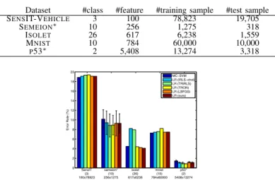
TABLE II. DATASETS OF DENSE FEATURES. WE APPLY FIVE-FOLD CROSS VALIDATION ON THE DATASETS MARKED BY∗,WHILE USING
GIVEN TRAINING/TEST SPLITS ON THE OTHER DATASETS. Dataset #class #feature #training sample #test sample SENSIT-VEHICLE 3 100 78,823 19,705
SEMEION∗ 10 256 1,275 318
ISOLET 26 617 6,238 1,559
MNIST 10 784 60,000 10,000
P53∗ 2 5,408 13,274 3,318
0 2 4 6 8 10 12 14 16 18 20
SensIT (3) 100x78823
semeion* (10) 256x1275
isolet (26) 617x6238
mnist (10) 784x60000
p53* (2) 5408x13274
Error Rate (%)
MC−SVM LR (IRLS−chol) LR (TRIRLS) LR (TRON) LR (LBFGS) LR (ours)
Fig. 1. Error rates on linear classification for dense features. The numbers of classes are indicated in parentheses and the sizes ofX (#feature×#sample) are shown in the bottom.
A. Linear classification
As a preliminary experiment to the subsequent kernel-based methods, we applied linear classification methods.
For comparison, we applied multi-class support vector machine (MC-SVM) [7] and for LR, four types of optimization methods other than the proposed method in Section III:
• IRLS with Cholesky decomposition (IRLS-chol) [17]
• IRLS with CG (TRIRLS) [18]
• IRLS with trust region newton method (TRON) [20]
• limited memory BFGS method (LBFGS) [13] and [21].
All of these methods introduce regularization with respect to classifier norm in a similar form to (3), of which the regularization parameter is determined by three-fold cross
validation on training samples (λ ∈ {1,10−2,10−4}). We
implemented all the methods by using MATLAB with C-mex
on Xeon 3GHz (12 threading) PC; we usedLIBLINEAR [32]
for MC-SVM and TRON, and the code1 provided by Liu and
Nocedal [22] for LBFGS.
We first used the datasets2 of the dense feature vectors,
the details of which are shown in Table II. For evaluation, we used the given training/test splits on some datasets and applied five-fold cross validation on the others. The classification per-formances (error rates) and the computation times for training the classifier are shown in Fig. 1 and Fig. 2, respectively. The computation times are measured in two ways; Fig. 2(a) shows the computation time only for learning the final classifier and Fig. 2(b) is for ‘whole’ training process including both the final learning and three-fold cross validations to determine the regularization parameter. The proposed method is favorably compared to the other methods in terms of error rates and computation time; the method of LR with IRLS-chol which is quite close to the ordinary IRLS requires more training time.
1The code is available at http://www.ece.northwestern.edu/∼nocedal.
2SEMEION, ISOLET and P53 are downloded from UCI-repository http://archive.ics.uci.edu/ml/datasets.html, and SENSIT-VEHICLE [33] and MNIST[34] are from http://www.csie.ntu.edu.tw/∼cjlin/libsvmtools/datasets/.
10−2 10−1 100 101 102 103
SensIT (3) 100x78823
semeion* (10) 256x1275
isolet (26) 617x6238
mnist (10) 784x60000
p53* (2) 5408x13274
Training Time (sec)
MC−SVM LR (IRLS−chol) LR (TRIRLS) LR (TRON) LR (LBFGS) LR (ours)
10−1 100 101 102 103 104 105
SensIT (3) 100x78823
semeion* (10) 256x1275
isolet (26) 617x6238
mnist (10) 784x60000
p53* (2) 5408x13274
Whole Training Time (sec)
MC−SVM LR (IRLS−chol) LR (TRIRLS) LR (TRON) LR (LBFGS) LR (ours)
(a) On final learning (b) On whole learning Fig. 2. Computation times (log-scale) on linear classification for dense features. The computation time for learning final classifier is shown in (a), while that for whole training including 3-CV to determineλis in (b).
0 100 200 300 400 500 600 700 800 900 102
103 104 105
Iteration
Cost
Ours (optimized α) Line search (Wolf condition)
Fig. 3. Comparison to the method using an exhaustive line search. The plot shows the objective cost values through iterations on ISOLET.
We then investigated the effectiveness of the optimized
step size α (Section III-B) which is one of our contributions
in this paper. Fig. 3 shows how the proposed optimization method works, compared to that using an exhaustive line search. By employing the optimized step size, the objective cost drastically decreases in the fist few steps and reaches convergence in a smaller number of iterations.
In the same experimental protocol, we also applied the methods to datasets which contain sparse feature vectors. The
details of the datasets3 are shown in Table III. Note that the
method of LR with IRLS-chol can not deal with such a huge feature vectors since the Hessian matrix is quite large, making it difficult to solve linear equations by Cholesky decomposition in a realistic time. As shown in Fig. 4 and Fig. 5, the computation times of the methods are all comparable (around 10 seconds) with similar classification accuracies.
Though the performances of the proposed method are favorably compared to the others as a whole, they are different from those of IRLS-based methods (TRIRLS and TRON). The
reason is as follows. The objective costs of those methods4
are shown in Table IV. The proposed method produces lower objective costs than those by TRIRLS, and thus we can say that the IRLS-based method does not fully converge to global minimum. Although the objective cost function is convex, there would exist plateau [38] which stop the optimization in the IRLS-based methods before converging to the global minimum. Thus, from the viewpoint of optimization, the proposed method produces favorable results.
3REUTERS21578 (UCI KDD Archive) and TDT2 (Nist Topic Detection and Tracking corpus) are downloaded from http://www.zjucadcg.cn/dengcai/ Data/TextData.html, and RCV1 [35], SECTOR[36] and NEWS20 [37] are from http://www.csie.ntu.edu.tw/∼cjlin/libsvmtools/datasets/.
4We do not show the cost of TRON [20] whose formulation is slightly different as described in Section II-A.
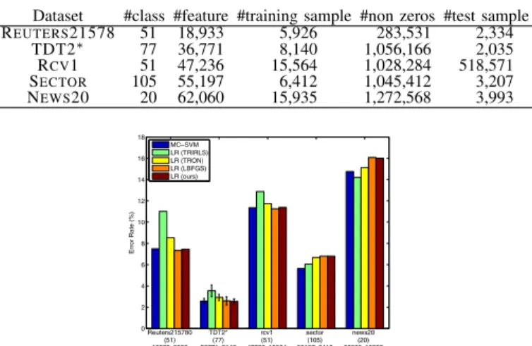
TABLE III. DATASETS OF SPARSE FEATURES. WE APPLY FIVE-FOLD CROSS VALIDATION ON THE DATASETS MARKED BY∗,WHILE USING
GIVEN TRAINING/TEST SPLITS ON THE OTHER DATASETS. Dataset #class #feature #training sample #non zeros #test sample REUTERS21578 51 18,933 5,926 283,531 2,334
TDT2∗ 77 36,771 8,140 1,056,166 2,035
RCV1 51 47,236 15,564 1,028,284 518,571 SECTOR 105 55,197 6,412 1,045,412 3,207 NEWS20 20 62,060 15,935 1,272,568 3,993
0 2 4 6 8 10 12 14 16 18
Reuters215780 (51) 18933x5926
TDT2* (77) 36771x8140
rcv1 (51) 47236x15564
sector (105) 55197x6412
news20 (20) 62060x15935
Error Rate (%)
MC−SVM LR (TRIRLS) LR (TRON) LR (LBFGS) LR (ours)
Fig. 4. Error rates on linear classification for sparse features.
B. Kernel-based classification
Next, we conducted the experiments on kernel-based clas-sifications. We applied the proposed kernel logistic regression (KLR) in Section IV and the kernelized methods of the above-mentioned linear classifiers;
• multi-class kernel support vector machine (MC-KSVM) [7]
• KLR using IRLS with CG (TRIRLS) [18]
• KLR using IRLS with trust region newton method (TRON)
by [20]
• KLR using limited memory BFGS method (LBFGS) [13],
[21].
Note that the KLR methods of TRIRLS, TRON and LBFGS are kernelized in the way described in Section II-D. Table V
shows the details of the datasets5 that we use, and in this
ex-periment, we employed RBF kernelk(x,ξ) = exp(−x2−σξ22)
where σ2 is determined as the sample variance. The
experi-mental protocol is the same as in Section VII-A.
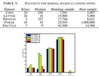
As shown in Fig. 6, the classification performances of the proposed method are superior to the other KLR methods and are comparable to MC-KSVM, while the computation times of the proposed method are faster than that of MC-KSVM on most datasets (Fig. 7). As discussed in Section VI, we can employ GPGPU (NVIDIA Tesla C2050) to efficiently compute the matrix multiplications in our method on the datasets except
for the huge dataset of SHUTTLE, and the computation time
is significantly reduced as shown in Fig. 7.
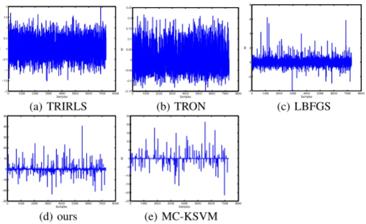
While the proposed method optimizes the classifier in RKHS, the optimization in the other KLR methods is per-formed in the subspace spanned by the sample kernel functions (Section IV), possibly causing numerically unfavorable issues such as plateau [38], and the optimizations would terminate before fully converging to the global minimum. The objective costs shown in Table VI illustrates it; the proposed method provides lower costs than those of the other KLR methods.
In addition, the obtained classifiers, i.e., coefficients W for
5USPS[39], LETTER(Statlog), PROTEIN[40] and SHUTTLE(Statlog) are downloaded from http://www.csie.ntu.edu.tw/∼cjlin/libsvmtools/datasets/, and POKERis from UCI repository http://archive.ics.uci.edu/ml/datasets/.
10−1 100 101 102
Reuters215780 (51) 18933x5926
TDT2* (77) 36771x8140
rcv1 (51) 47236x15564
sector (105) 55197x6412
news20 (20) 62060x15935
Training Time (sec)
MC−SVM LR (TRIRLS) LR (TRON) LR (LBFGS) LR (ours)
100 101 102 103 104
Reuters215780 (51) 18933x5926
TDT2* (77) 36771x8140
rcv1 (51) 47236x15564
sector (105) 55197x6412
news20 (20) 62060x15935
Whole Training Time (sec)
MC−SVM LR (TRIRLS) LR (TRON) LR (LBFGS) LR (ours)
(a) On final learning (b) On whole learning Fig. 5. Computation times on linear classification for sparse features.
TABLE IV. OBJECTIVE COST VALUES OFLRMETHODS WITH λ= 10−2ON SPARSE DATASETS.
Dataset Ours TRIRLS LBFGS
REUTERS21578 9.98 389.26 10.32 TDT2 12.13 387.58 13.65 RCV1 906.49 15687.17 969.07 SECTOR 1102.08 29841.19 1167.35 NEWS20 1949.60 7139.07 2000.64
samples, are shown in Fig. 8. The proposed method produces near sparse weights compared to those of the other methods and contribute to improve the performance similarly to MC-KSVM, even though any constraints to enhance sparseness are not imposed in the proposed method.
C. Multiple-kernel learning
Finally, we conducted the experiment on multiple-kernel learning. We applied the proposed multiple-kernel logistic re-gression (MKLR) described in Section V and simpleMKL [29]
for comparison. For simpleMKL, we used the code6 provided
by the author with LIBSVM[41]. The details of the datasets7
are shown in Table VII; for multi-class classification, in the
dataset of PASCAL-VOC2007, we removed the samples to
which multiple labels are assigned. In the datasets of PSORT-,
NONPLANTand PASCAL-VOC2007, we used the precomputed kernel matrices provided in the authors’ web sites. The dataset of PEN-DIGITS contains four types of feature vectors and correspondingly we constructed four types of RBF kernel in the same way as in Section VII-B.
The classification performances are shown in Fig. 9. As a reference, we also show the performances of KLR with the (single) averaged kernel matrix and the (single) best kernel matrix which produces the best performance among the multiple kernel matrices. The MKL methods produce superior performances compared to those of KLR with single kernel, and the proposed method is comparable to simpleMKL. The obtained kernel weights are also shown in Fig. 10. The weights by the proposed method are sparse similarly to those by simpleMKL, due to the formulation based on the combined
RKHSH¯in (14) and its efficient optimization using non-linear
CG.
As shown in Fig. 11, the computation time of the
pro-posed method is significantly (102 ∼ 104 times) faster than
6The code is available at http://asi.insa-rouen.fr/enseignants/∼arakotom/ code/mklindex.html
TABLE V. DATASETS FOR KERNEL-BASED CLASSIFICATION. Dataset #class #feature #training sample #test sample
USPS 10 256 7,291 2,007
LETTER 26 16 15,000 5,000
PROTEIN 3 357 17,766 6,621
POKER 10 10 25,010 1,000,000
SHUTTLE 7 9 43,500 14,500
0 5 10 15 20 25 30 35 40 45 50
usps (10) 7291x7291
letter (26) 15000x15000
protein (3) 17766x17766
poker (10) 25010x25010
shuttle (7) 43500x43500
Error Rate (%)
MC−KSVM KLR (TRIRLS) KLR (TRON) KLR (LBFGS) KLR (ours)
Fig. 6. Error rates on kernel-based classification.
that of simpleMKL. Thus, as is the case with kernel-based classification (Section VII-B), we can say that the proposed method produces comparable performances to simpleMKL with a significantly faster training time.
VIII. CONCLUDINGREMARKS
In this paper, we have proposed an efficient optimization method using non-linear conjugate gradient (CG) descent for logistic regression. The proposed method efficiently minimizes the cost through CG iterations by using the optimized step size without an exhaustive line search. On the basis of the non-linear CG based optimization scheme, a novel optimization method for kernel logistic regression (KLR) is also proposed. Unlike the ordinary KLR methods, the proposed method naturally formulates the classifier as the linear combination of sample kernel functions and directly optimizes the kernel-based classifier in the reproducing kernel Hilbert space, not the linear coefficients for the samples. Thus, the optimization effectively performs while possibly avoiding the numerical issues such as plateau. We have further developed the KLR using single kernel to multiple-kernel LR (MKLR). The pro-posed MKLR, which is also optimized in the scheme of non-linear CG, produces the kernel-based classifier with optimized weights for multiple kernels. In the experiments on various multi-class classification tasks, the proposed methods produced favorable results in terms of classification performance and computation time, compared to the other methods.
REFERENCES
[1] G. Wang, D. Hoiem, and D. Forsyth, “Building text features for object image classification,” in IEEE Conference on Computer Vision and Pattern Recognition, 2009, pp. 1367–1374.
[2] S. K. Divvala, D. Hoiem, J. H. Hays, A. A. Efros, and M. Hebert, “An empirical study of context in object detection,” inIEEE Conference on Computer Vision and Pattern Recognition, 2009, pp. 1271–1278. [3] I. Laptev, M. Marszaek, C. Schmid, and B. Rozenfeld, “Learning
realistic human actions from movies,” inIEEE Conference on Computer Vision and Pattern Recognition, 2008.
[4] A. Genkin, D. D. Lewis, and D. Madigan, “Large-scale bayesian logistic regression for text categorization,” Technometrics, vol. 49, no. 3, pp. 291–304, 2007.
[5] P. J. Bartlett, B. Sch¨olkopf, D. Schuurmans, and A. J. Smola, Eds., Advances in Large-Margin Classifiers. MIT Press, 2000.
100 101 102 103 104 105
usps (10) 7291x7291
letter (26) 15000x15000
protein (3) 17766x17766
poker (10) 25010x25010
shuttle (7) 43500x43500
Training Time (sec)
MC−KSVM KLR (TRIRLS) KLR (TRON) KLR (LBFGS) KLR (ours) KLR (ours−gpu)
101 102 103 104 105 106
usps (10) 7291x7291
letter (26) 15000x15000
protein (3) 17766x17766
poker (10) 25010x25010
shuttle (7) 43500x43500
Whole Training Time (sec)
MC−KSVM KLR (TRIRLS) KLR (TRON) KLR (LBFGS) KLR (ours) KLR (ours−gpu)
(a) On final learning (b) On whole learning Fig. 7. Computation times on kernel-based classification.
TABLE VI. OBJECTIVE COST VALUES OFKLRMETHODS WITH λ= 10−2ON KERNEL DATASETS.
Dataset Ours TRIRLS LBFGS
USPS 446.37 914.88 501.15 LETTER 4746.13 12476.41 5789.30 PROTEIN 5866.16 12576.97 10650.96 POKER 22186.19 30168.74 23345.94 SHUTTLE 759.99 1100.07 811.91
[6] V. Vapnik,Statistical Learning Theory. Wiley, 1998.
[7] K. Crammer and Y. Singer, “On the algorithmic implementation of multiclass kernel-based vector machines,”Journal of Machine Learning Research, vol. 2, pp. 265–292, 2001.
[8] J. Platt, “Fast training of support vector machines using sequential minimal optimization,” inAdvances in Kernel Methods - Support Vector Learning, B. Sch¨olkopf, C. Burges, and A. Smola, Eds. Cambridge, MA, USA: MIT Press, 1999, pp. 185–208.
[9] J. Nocedal and S. Wright,Numerical Optimization. Springer, 1999. [10] W. W. Hager and H. Zhang, “A survey of nonlinear conjugate gradient
methods,”Pacific Journal of Optimization, vol. 2, pp. 35–58, 2006. [11] G. Lanckriet, N. Cristianini, P. Bartlett, L. E. Ghaoui, and M. I. Jordan,
“Learning the kernel matrix with semidefinite programming,”Journal of Machine Learning Research, vol. 5, pp. 27–72, 2004.
[12] K. Watanabe, T. Kobayashi, and N. Otsu, “Efficient optimization of logistic regression by direct cg method,” in International Conference on Machine Learning and Applications, 2011.
[13] R. Malouf, “A comparison of algorithms for maximum entropy parame-ter estimation,” inThe Sixth Conference on Natural Language Learning, 2002, pp. 49–55.
[14] C. Sutton and A. McCallum,An introduction to conditional random fields for relational learning, L. Getoor and B. Taskar, Eds. MIT Press, 2006.
[15] T. Minka, “A comparison of numerical optimizers for logistic regres-sion,” Carnegie Mellon University, Technical report, 2003.
[16] C. M. Bishop,Pattern Recognition and Machine Learning. Springer, 2007.
[17] P. Komarek and A. Moore, “Fast robust logistic regression for large sparse datasets with binary outputs,” inThe 9th International Workshop on Artificial Intelligence and Statistics, 2003, pp. 3–6.
[18] ——, “Making logistic regression a core data mining tool,” in Interna-tional Conference on Data Mining, 2005, pp. 685–688.
[19] M. R. Hestenes and E. L. Stiefel, “Methods of conjugate gradients for solving linear systems,”Journal of Research of the National Bureau of Standards, vol. 49, no. 6, pp. 409–436, 1952.
[20] C.-J. Lin, R. Weng, and S. Keerthi, “Trust region newton methods for large-scale logistic regression,” inInternational Conference on Machine Learning, 2007, pp. 561–568.
[21] H. Daum´e III, “Notes on CG and LM-BFGS optimization of logistic regression,” Technical report, 2004. [Online]. Available: http://www.umiacs.umd.edu/∼hal/docs/daume04cg-bfgs.pdf
[22] D. C. Liu and J. Nocedal, “On the limited memory bfgs method for large scale optimization,”Mathematical Programming, vol. 45, pp. 503–528, 1989.
[23] S. D. Pietra, V. D. Pietra, and J. Lafferty, “Inducing features of
0 1000 2000 3000 4000 5000 6000 7000 8000 −2
−1.5 −1 −0.5 0 0.5 1 1.5 2
Samples
W
0 1000 2000 3000 4000 5000 6000 7000 8000 −0.15
−0.1 −0.05 0 0.05 0.1 0.15 0.2 0.25
Samples
W
0 1000 2000 3000 4000 5000 6000 7000 8000 −4
−2 0 2 4 6 8
Samples
W
(a) TRIRLS (b) TRON (c) LBFGS
0 1000 2000 3000 4000 5000 6000 7000 8000 −30
−20 −10 0 10 20 30 40 50
Samples
W
0 1000 2000 3000 4000 5000 6000 7000 8000 −25
−20 −15 −10 −5 0 5 10 15 20 25
Samples
W
(d) ours (e) MC-KSVM
Fig. 8. Classifiers (coefficientsw1across samples) of class 1 on USPS. TABLE VII. DATASETS FOR MULTIPLE-KERNEL LEARNING. WE APPLY
FIVE-FOLD CROSS VALIDATION ON THE DATASETS MARKED BY∗,WHILE USING GIVEN TRAINING/TEST SPLITS ON THE OTHER DATASETS.
Dataset #class #kernel #training sample #test sample
PSORT-∗ 5 69 1,155 289
NONPLANT∗ 3 69 2,186 546
PASCAL-VOC2007 20 15 2,954 3,192
PEN-DIGITS 10 4 7,494 3,498
random fields,” IEEE Transactions on Pattern Analysis and Machine Intelligence, vol. 19, no. 4, pp. 380–393, 1997.
[24] J. Zhu and T. Hastie, “Kernal logistic regression and the import vector machine,”Journal of Computational and Graphical Statistics, vol. 14, no. 1, pp. 185–205, 2005.
[25] G. Wahba, C. Gu, Y. Wang, and R. Chappell, “Soft classification, a.k.a. risk estimation, via penalized log likelihood and smoothing spline analysis of variance,” in The Mathematics of Generalization, D. Wolpert, Ed. Reading, MA, USA: Addison-Wesley, 1995, pp. 329– 360.
[26] T. Hastie and R. Tibshirani,Generalized Additive Models. Chapman and Hall, 1990.
[27] B. Sch¨olkopf and A. Smola,Learning with Kernels. MIT Press, 2001. [28] Y. Dai and L. Liao, “New conjugacy conditions and related nonlinear conjugate gradient methods,” Applied Mathmatics and Optimization, vol. 43, pp. 87–101, 2001.
[29] A. Rakotomamonjy, F. R. Bach, S. Canu, and Y. Grandvalet, “Sim-plemkl,”Journal of Machine Learning Research, vol. 9, pp. 2491–2521, 2008.
[30] F. Bach, “Consistency of the group lasso and multiple kernel learning,” Journal of Machine Learning Research, vol. 9, pp. 1179–1225, 2008. [31] J. Bonnans, J. Gilbert, C. Lemar´echal, and C. Sagastiz´abal,Numerical
Optimization: Theoritical and Practical Aspects. Springer, 2006. [32] R. Fan, K. Chang, C. Hsieh, X. Wang, and C. Lin, “Liblinear: A library
for large linear classificatio,” Journal of Machine Learning Research, vol. 9, pp. 1871–1874, 2008, Software available at http://www.csie.ntu. edu.tw/∼cjlin/liblinear.
[33] M. Duarte and Y. H. Hu, “Vehicle classification in distributed sensor networks,” Journal of Parallel and Distributed Computing, vol. 64, no. 7, pp. 826–838, 2004.
[34] Y. LeCun, L. Bottou, Y. Bengio, and P. Haffner, “Gradient-based learning applied to document recognition,” Proceedings of the IEEE, vol. 86, no. 11, pp. 2278–2324, 1998.
[35] D. D. Lewis, Y. Yang, T. G. Rose, and F. Li, “Rcv1: A new bench-mark collection for text categorization research,” Journal of Machine Learning Research, vol. 5, pp. 361–397, 2004.
[36] A. McCallum and K. Nigam, “A comparison of event models for naive bayes text classification,” inAAAI’98 Workshop on Learning for Text categorization, 1998.
[37] K. Lang, “Newsweeder: Learning to filter netnews,” in International Conference on Machine Learning, 1995, pp. 331–339.
[38] K. Fukumizu and S. Amari, “Local minima and plateaus in hierarchical
0 10 20 30 40 50 60
psort−* (5) 1156x1156x69
nonplant* (3) 2186x2186x69
PASCAL2007 (20) 2954x2954x15
pendigits (10) 7494x7494x4
Error Rate (%)
KLR (best) KLR (average) simpleMKL MKLR (ours)
Fig. 9. Error rates and computation times on multiple-kernel learning.
1 2 3 4 5 6 7 8 9 10 11 1213 14 15 0
0.1 0.2 0.3 0.4 0.5 0.6 0.7
Kernels
v
1 2 3 4 5 6 7 8 9 10 1112 1314 15 0
0.05 0.1 0.15 0.2 0.25 0.3 0.35 0.4
Kernels
v
(a) simpleMKL [29] (b) MKLR (ours) Fig. 10. The obtained kernel weightsvon PASCAL-VOC2007.
100 101 102 103 104 105 106
psort−* (5) 1156x1156x69
nonplant* (3) 2186x2186x69
PASCAL2007 (20) 2954x2954x15
pendigits (10) 7494x7494x4
Training Time (sec)
simpleMKL MKLR (ours)
100 101 102 103 104 105 106 107
psort−* (5) 1156x1156x69
nonplant* (3) 2186x2186x69
PASCAL2007 (20) 2954x2954x15
pendigits (10) 7494x7494x4
Whole Training Time (sec)
simpleMKL MKLR (ours)
(a) On final learning (b) On whole learning Fig. 11. Computation times on multiple-kernel learning.
structures of multilayer perceptrons,”Neural Networks, vol. 13, no. 3, pp. 317–327, 2000.
[39] J. Hull, “A database for handwritten text recognition research,” IEEE Transactions on Pattern Analysis and Machine Intelligence, vol. 16, no. 5, pp. 550–554, 1994.
[40] J.-Y. Wang, “Application of support vector machines in bioinformatics,” Master’s thesis, Department of Computer Science and Information Engineering, National Taiwan University, 2002.
[41] C.-C. Chang and C.-J. Lin, LIBSVM: a library for support vector machines, 2001, software available at http://www.csie.ntu.edu.tw/∼cjlin/ libsvm.
[42] M. Guillaumin, J. Verbeek, and C. Schmid, “Multimodal semi-supervised learning for image classification,” in IEEE Conference on Computer Vision and Pattern Recognition, 2010, pp. 902–909. [43] F. Alimoglu and E. Alpaydin, “Combining multiple representations and