www.atmos-meas-tech.net/9/5707/2016/ doi:10.5194/amt-9-5707-2016
© Author(s) 2016. CC Attribution 3.0 License.
A high-altitude balloon platform for determining exchange of
carbon dioxide over agricultural landscapes
Angie Bouche1, Bernhard Beck-Winchatz2, and Mark J. Potosnak1
1Department of Environmental Science and Studies, DePaul University, 1110 W Belden Ave,
Chicago, IL, 60614, USA
2Department of Science, Technology, Engineering and Math Studies, DePaul University,
990 W Fullerton Ave, Chicago, IL, 60614, USA
Correspondence to:Mark J. Potosnak ([email protected])
Received: 14 March 2016 – Published in Atmos. Meas. Tech. Discuss.: 11 May 2016 Revised: 2 November 2016 – Accepted: 2 November 2016 – Published: 29 November 2016
Abstract.The exchange of carbon dioxide between the ter-restrial biosphere and the atmosphere is a key process in the global carbon cycle. Given emissions from fossil fuel com-bustion and the appropriation of net primary productivity by human activities, understanding the carbon dioxide ex-change of cropland agroecosystems is critical for evaluating future trajectories of climate change. In addition, human ma-nipulation of agroecosystems has been proposed as a tech-nique of removing carbon dioxide from the atmosphere via practices such as no-tillage and cover crops. We propose a novel method of measuring the exchange of carbon diox-ide over croplands using a high-altitude balloon (HAB) plat-form. The HAB methodology measures two sequential ver-tical profiles of carbon dioxide mixing ratio, and the surface exchange is calculated using a fixed-mass column approach. This methodology is relatively inexpensive, does not rely on any assumptions besides spatial homogeneity (no horizontal advection) and provides data over a spatial scale between sta-tionary flux towers and satellite-based inversion calculations. The HAB methodology was employed during the 2014 and 2015 growing seasons in central Illinois, and the results are compared to satellite-based NDVI values and a flux tower located relatively near the launch site in Bondville, Illinois. These initial favorable results demonstrate the utility of the methodology for providing carbon dioxide exchange data over a large (10–100 km) spatial area. One drawback is its relatively limited temporal coverage. While recruiting citizen scientists to perform the launches could provide a more ex-tensive dataset, the HAB methodology is not appropriate for providing estimates of net annual carbon dioxide exchange.
Instead, a HAB dataset could provide an important check for upscaling flux tower results and verifying satellite-derived exchange estimates.
1 Introduction
for understanding the global carbon cycle. This has led to an interest in understanding the impact of agricultural practices, such as no-tillage, on the net carbon balance of agricultural systems, but experimental results are often conflicting (Luo et al., 2010) and point to the need for diverse measurement strategies of the carbon balance of agricultural landscapes.
Measuring the net ecosystem exchange (NEE) of carbon dioxide for agroecosystems can show whether agricultural practices are an effective way to offset some of the carbon dioxide that was released into the atmosphere through an-thropogenic causes. Considering annual crops, agricultural practices that increase soil organic carbon (SOC) remove carbon dioxide from the atmosphere (here defined as nega-tive NEE), neglecting any carbon flows through hydrologi-cal systems. While there is debate about the effectiveness of no-tillage farming (Hollinger et al., 2005; Luo et al., 2010), cover crops are another method being considered for in-creasing SOC (Poeplau and Don, 2015). The effectiveness of these practices can be constrained by measuring the NEE of carbon dioxide between agricultural systems and the atmo-sphere. Surface–atmosphere exchange measurements com-plement methodologies that assess the change in SOC to de-termine agroecosystem carbon balance. A variety of strate-gies have been employed to measure carbon dioxide fluxes in an effort to understand these exchanges.
Data collected with towers, satellites and airplanes have been used to quantify fluxes of carbon dioxide. The eddy covariance (EC) approach employs instruments mounted on towers to measure NEE over areas on the order of 1 km2 (Monson and Baldocchi, 2014). In combination with chemi-cal tracers, these flux measurements can be used to infer an-thropogenic and biogenic influences on carbon dioxide mix-ing ratios over wider areas (Potosnak et al., 1999). However, there is not a large amount of data available that measure car-bon dioxide exchanges in agricultural areas using this tech-nique (Barcza et al., 2009). Surface measurements of carbon dioxide mixing ratio from a global network can be combined with atmospheric transport models and a priori estimates of anthropogenic and oceanic carbon dioxide exchanges to pro-duce regional estimates of biotic carbon dioxide exchange (Enting et al., 1995; Gurney et al., 2002). These efforts have produced important results at the regional scale (Peters et al., 2007), but they do rely on an imperfect measurement net-work, estimated a priori sources and complex transport mod-els (Gurney et al., 2004).
Collecting data via satellites and performing inverse mod-els is another way to measure carbon dioxide fluxes over ar-eas of land on the order of 107km2, but again there is not a large body of data available and there are significant mea-surement uncertainties (Reuter et al., 2014). Progress is be-ing made by usbe-ing satellite data to constrain carbon diox-ide exchanges at the scale of large urban areas, but efforts currently focus on atmospheric mixing ratio enhancements and not exchanges (Schneising et al., 2013). New approaches using solar-induced fluorescence derived from satellite
mea-surements to predict crop productivity are promising (Guan et al., 2016), but these will require validation. An alterna-tive approach is to perform a budget of carbon dioxide in the mixed layer. With some assumptions, the surface flux of car-bon dioxide can be calculated from vertical profiles of carcar-bon dioxide mixing ratio in the mixed layer.
This long-standing technique was employed with aircraft in the Amazon during the 1980s (Wofsy et al., 1988), and the theory was thoroughly considered during the 1990s (Den-mead et al., 1996). Measurement efforts using aircraft con-tinue (Chou et al., 2002; Martins et al., 2009), along with fur-ther advances in theoretical treatment (Laubach and Fritsch, 2002). While the technique is robust, the expense of air-craft is considerable. An alternative involves carbon diox-ide sensors flown on high-altitude balloons (HABs). Given assumptions detailed below, HABs can measure surface ex-change by comparing mixing ratio profiles between two se-quential flights and performing a mass-balance calculation. HABs are able to collect data at an intermediate scale be-tween the small-scale measurements collected by towers and large-scale measurements collected using satellites. The spa-tial scale is similar to aircraft measurements (Mays et al., 2009), but the cost is much lower. This paper describes fly-ing an in situ instrument, but another proposed technique that could use HABs is AirCore. This simple sampling device is also low cost and has been tested with an aircraft platform (Karion et al., 2010). Some drawbacks to the mixed-layer budget approach are limited temporal resolution and the re-quirement of spatial homogeneity.
NDVI decreases throughout this process as leaf chlorophyll content decreases during senescence. In the winter after har-vest, NDVI is lowest since bare ground is exposed. These seasonal trends should mirror trends in NEE. Moving from spring to summer, NEE becomes negative because crops are growing and photosynthesis exceeds total respiration. NEE is most negative in the middle of summer when plants are con-ducting photosynthesis rapidly. When crops are left in the field to dry or are harvested, NEE is expected to be positive because crops are not conducting photosynthesis or growing, while the soil is still respiring.
To assess the quality of NEE measured with the HAB plat-form, 2 years of growing-season results are compared to the satellite-derived NDVI values from an area representative of the HAB footprint. Based on the argument outlined in the previous paragraph, we hypothesized that the HAB NEE val-ues should follow the same seasonal pattern as NDVI if the method is effective. In addition, the magnitude of the NEE values measured with the HAB platform are compared to publicly available data from a EC flux site.
2 Materials and methods
Measuring NEE can be accomplished by comparing verti-cal profiles of carbon dioxide mixing ratios from two HAB launches 3–4 h apart. We followed the fixed-mass column ap-proach outlined by Laubach and Fritsch (2002). Compared to using the variable mixed-layer height, this approach has some advantages for calculating the contribution of entrain-ment in the budget, because there are fewer assumptions about the structure and evolution of the vertical profile of car-bon dioxide in the free troposphere. The technique is based on estimating the boundary layer height for both flights and also considering changes in the density of the air column. The mass of the column is calculated by integrating air den-sity from the surface to both the initial and the final boundary layer heights. The larger of these two masses is then selected for the budget, which is typically the mass of the final flight during conditions when the mixed-layer height is growing. If there is little or no observable growth, the initial flight can have the larger mass since thermal expansion of the mixed layer leads to lower densities for the final flight. This calcu-lated mass is then used for both flights (Laubach and Fritsch, 2002, Eqs. 30 and 31). With the fixed mass, the column ex-change of carbon dioxide (including entrainment but not sub-sidence) is then calculated by comparing the vertical spatial average of the carbon dioxide mixing ratios between the two flights (Eq. 33 in Laubach and Fritsch and also included in Eq. 2 below). When the average carbon dioxide mixing ratio is higher for the first flight than the second, carbon dioxide is being removed from the atmosphere (defined as negative NEE and corresponding to photosynthesis exceeding respira-tion). Similar to the EC technique, this method assumes that net horizontal advection is negligible and therefore requires
360 370 380
500
1000
1500
2000
2500
3000
CO2 (ppm)
● ● ● ● ● ● ● ● ● ● ● ● ● ● ● ● ● ● ● ●
● Flight 1
Flight 2
∆CO2 (ppmvh−1)
Idealized flight
−7 −6 −5 −4 −3 −2
A
lt
it
u
d
e
(
m
)
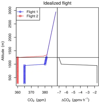
Figure 1.An idealized flight that includes a well-mixed, homoge-neous mixing ratio of carbon dioxide near ground level, then a de-crease in carbon dioxide mixing ratio from the first launch (blue) to second launch (red) corresponding with an increase in the bound-ary layer height. Above the boundbound-ary layer height of the second flight, mixing ratios between the flights should match again because ground-level photosynthetic activity does not affect carbon dioxide mixing ratios above this altitude (left panel). Both the decrease in the mixed-layer carbon dioxide mixing ratio and the increase in the
boundary layer height contribute to1CO2, and hence NEE. This
idealized picture neglects subsidence and horizontal advection.
spatial homogeneity across the area being studied. To put a practical limit on the assumption of horizontal homogeneity, the relevant changes in carbon dioxide are assumed to be in the boundary layer, which is defined as the layer of the tro-posphere affected by surface exchanges within a timescale of 1 h or less (Stull, 1988). The method does rely on a knowl-edge of the boundary layer height. During the daytime in the summer, the atmosphere is approximately homogeneous in its carbon dioxide mixing ratio within the boundary layer be-cause it is mixed by convection and turbulence (the mixed layer; Stull, 1988). Above the mixed layer, at an altitude of approximately 1000–2000 m, there is a large increase in car-bon dioxide mixing ratio over a relatively short change in al-titude (the entrainment zone) that can be visually identified. The mixed-layer height typically increases for the second flight due to increased vertical mixing driven by additional solar heating at the surface (Fig. 1). Above the mixed-layer height, the two carbon dioxide profiles should be similar, and differences would be due to changes in large-scale horizontal advection and subsidence.
dif-ference in carbon dioxide values recorded during the ascent and descent of a single flight. In the previous methodology, the launch site and retrieval site could have different surface characteristics that could affect carbon dioxide mixing ratios in the surface layer. Therefore, using two ascents for com-parison removed an aspect of spatial heterogeneity. The ad-ditional time between flights, when compared to the time be-tween ascent and descent of a single flight (less than 1 h), also allowed for a larger difference in carbon dioxide mixing ratio and a greater increase in the boundary layer height.
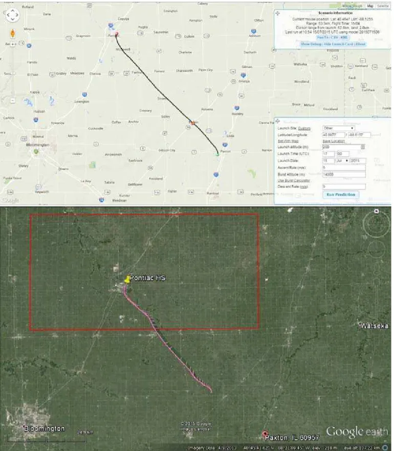
Throughout the summers of 2014 and 2015, a total of 10 launches were performed. Four of these launches took place from July to September 2014, and six took place from June to September 2015 (Table 1). As the balloon ascended, burst and descended, it was followed by a chase vehicle us-ing GPS location data received from the trackus-ing devices. Once the balloon was retrieved, the process was repeated approximately 3 h later. The launches took place at an ath-letic field at Pontiac Township High School in Pontiac, IL (40.886◦N, 88.616◦W), with the exception of the flight on 17 July 2014, which took place at Koerner Aviation in Kankakee, IL (41.096◦N, 87.913◦W). Both of these loca-tions were small towns surrounded by agricultural fields of soy and corn crops, broken into the typical pattern of 2.6 km2 sections.
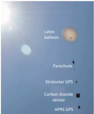
The equipment launched during each flight (Fig. 2) con-sisted of a latex balloon filled with helium, a parachute, two GPS tracking devices, a carbon dioxide sensor and an ozone sensor (2015 flights only). The ozone data were collected for another project to measure surface ozone exchange. The parachute (Rocketman Enterprise, Inc., Bloomington, MN, USA) had a spreader (wooden ring) and was above the Stratostar GPS command module (Noblesville, IN, USA). The command module was the primary source for tracking the location of the balloon, including the altitude provided by GPS. It also collected data on pressure, which was used to align the carbon dioxide data to the Stratostar GPS data. These data were relayed in real time to the chase vehicle via a 900 MHz radio signal. Carbon dioxide molar mixing ra-tios (ppmv) were obtained with a LICOR LI-820 (Lincoln, NE, USA). Ambient air was pumped through an air filter and then the carbon dioxide measuring device. The instru-ment was powered by 10 lithium AA disposable batteries. The instrument also reported cell pressure and temperature (controlled to 50◦C). Because of the relatively slow flow rate
(< 1 L min−1) and lack of restriction on the instrument outlet,
cell pressure was assumed to be equal to ambient pressure. The LI-820 is an infrared gas analyzer (IRGA), and therefore directly measures the optical absorptance of carbon dioxide in the cell. The instrument’s software uses the measured cell pressure and the assumption of a controlled temperature to convert absorptance to a mixing ratio (i.e., mole fraction). The air was not dried, so there is some error introduced if humidity changes between the flights (see error analysis). On the 19 June, 2 and 15 July 2015 flights, a LICOR LI-840 was
Latex alloon
Para hute
Stratostar GPS
Car on dioxide sensor
APRS GPS
Figure 2.Picture of flight train of packages. The total package weight of 5.4 kg was lifted by a 200 g latex balloon that was filled with industrial-grade helium. The packages were all connected with 1.8 m lines (mason’s string), except for 5.5 m lines for the balloon to parachute connection.
used. This instrument enabled us to also measure water vapor mixing ratios, which were used to understand the structure of the boundary layer and the impact of water vapor dilution. The two IRGAs were calibrated for carbon dioxide with a zero and a two-point calibration. After the instrument was ze-roed, the higher calibration standard (510.0 ppmv) was used to set the span, and then the calibration was checked with the lower calibration standard (372.4 ppmv). Standards were obtained from Airgas Specialty Gases (Chicago, IL, USA).
The data were collected from the LICOR instrument se-rial output using an Arduino (http://www.arduino.cc/) mi-crocontroller system and a memory card. A backup analog data logger (HOBO U12, Onset, Bourne, MA, USA) that recorded only carbon dioxide and pressure from the LICOR was also used. Finally, another GPS tracker (BigRedBee, Lake Oswego, OR, USA) was attached to the LICOR flight package and was used as a secondary tracking device that sent location data via a network of amateur ham radio op-erators to a website (Automatic Packet Reporting System, http://aprs.org/).
Table 1.Flight data from all flights conducted during the summers of 2014 and 2015. Each date had two separate flights to produce one estimate of NEE.
Date Burst altitude 1 Ascent rate 1 Burst altitude 2 Ascent rate 2
(m) (m s−1) (m) (m s−1)
17 Jul 2014 14 770 4.99 13 480 6.75
14 Aug 2014 15 000 5.16 14 810 5.49
21 Aug 2014 14 760 6.04 15 530 6.24
19 Sep 2014 13 290 6.34 13 850 5.52
19 Jun 2015 14 200 4.70 13 060 4.81
02 Jul 2015 13 030 5.37 13 730 5.10
15 Jul 2015 12 340 6.07 13 450 5.89
23 Jul 2015 12 930 5.93 12 490 6.40
13 Aug 2015 13 810 6.40 13 200 6.38
12 Sep 2015 9040 6.21 9400 5.21
grade helium until it obtained approximately 5 kg of lift, which produced an initial ascent rate of approximately 5– 6 m s−1 for our payload weight of 3.6 kg. In 2015, the bal-loon was filled until it obtained 7–8 kg of lift. It was neces-sary to obtain more lift on 2015 launches because an extra ozone sensor (1.8 kg) was attached to the flight package, giv-ing a total weight of 5.4 kg. On the 12 September 2015 flight, a 150 g balloon was used. Typically the balloons reached an altitude of around 13 000–15 000 m before bursting, but by using the smaller 150 g balloon on the 12 September 2015 flight the burst altitude was reduced to approximately 9000 m (Table 1).
The data were analyzed using R (version 3.3.1, R Core Team, 2016). To calculate a surface exchange from the mea-sured carbon dioxide profiles, the fixed-mass column ap-proach was applied. Some simplifications were employed due to the nature of the low-cost, low-weight flight package. The errors associated with this simplified approach are con-sidered in Sect. 3. All data were averaged by altitude into 50 m bins with the first bin at 300–350 m (the launch sites were at an elevation of approximately 230 m; everything ref-erenced to height above mean sea level) and the last bin at 2950–3000 m.
Because air temperature (T, K) is required for the fixed-mass column approach to find the air density (ρ, kg m−3) but was not directly measured with the low-cost flight pack-age, we computed the potential temperature (2) under the assumption that potential temperature was constant in the mixed layer. The profile of pressure (P, Pa) vs. the GPS-estimated altitude (z, m) was used to calculate potential tem-perature and also the altitude (z◦), where air pressure was
equal to 100 kPa (P◦). Combining the definition of
poten-tial temperature (2=T
P◦
P
R/CP
) and the ideal gas law (P =ρRT), the hydrostatic equation (dP= −ρg dz) was in-tegrated to find
z=2×CP g
"P
P◦
R/CP −1
#
| {z }
Scaled pressure
+z◦, (1)
with the constants R, CP and g being the ideal gas constant
for dry air (287 J kg−1K−1), the specific heat capacity for dry air at constant pressure (1004 J kg−1K−1) and the
accelera-tion due to gravity (9.81 N kg−1), respectively. This equation
can also be derived from the definition of potential tempera-ture and assuming the dry adiabatic lapse rate. By scaling the observed pressure as indicated by the equation, a linear fit be-tween the altitude and the scaled pressure gives the potential temperature as the slope and the altitude where pressure is 100 kPa as the intercept. Using the calculated potential tem-perature and the average measured pressure, the density of air was found using the ideal gas law for each altitude bin.
Next, the integrated ground exchange between the two flights was calculated according to Eq. (43) in Laubach and Fritsch (2002), using the notation from that paper:
ISG=αS (2)
Mtop hsitop2− hsitop1
+1
2wtopρtop(1s2+1s1) (t2−t1)
,
whereISGis the integrated ground flux (µ mol m−2),αS
con-verts from mass to mole units (mol kg−1),Mtopis the
con-stant mass of the column (kg),hsitop1,2is the spatially
aver-aged mixing ratio of carbon dioxide at the beginning and end of the integration (ppmv),wtopis the vertical velocity due to
synoptic-scale meteorology (m s−1),ρ
topis the air density at
the top of the column,1sis the difference between the mix-ing ratio above the column and average column mixmix-ing ratio
stop− hsitop
and(t2−t1)is the change in time (s). The
an-gle operator (h i) denotes the vertical spatial average from 300 m to the top of the fixed-mass column.
variation of convention from Laubach and Fritsch,αS
con-verted the mass of the column to moles, so the final flux units were molar (µmol m−2s−1) instead of mass (mg m−2s−1).
The constant mass was calculated as described in the first paragraph of Sect. 2. Essentially, a fixed mass was selected from the larger of the two flight’s mixed-layer masses, as cal-culated from the vertical density profile and the mixed-layer height. The mixed-layer height was determined from inspec-tion of the carbon dioxide profiles for each flight. Note that we use the term height when we reference the mixed layer, but since the data were collected via GPS, strictly speaking the vertical coordinate is altitude referenced to sea level, not height above the ground. For hsitop1,2, the carbon dioxide
mixing ratio was averaged to the altitudes that were deter-mined for the fixed mass. For one altitude, this is the top mixed-layer height, for the other flight, the altitude is deter-mined from the equivalent mass calculation.
The second term on the right-hand side of Eq. (2) ac-counts for synoptic-scale subsidence. The subsidence veloc-ity (wtop) was determined from the National Center for
En-vironmental Prediction’s North American Regional Reanal-ysis composites (http://www.esrl.noaa.gov/psd/cgi-bin/data/ narr/plothour.pl). Omega (Pa s−1) at 70 kPa and 18:00 GMT was converted to a vertical velocity using the air tempera-ture from the same data source, the ideal gas law and the hydrostatic equation (wtop= −/ (ρg)). The density (ρtop)
was calculated by averaging the density at the top of the mixed-layer mass for the two flights. The1s term depends on the averaged carbon dioxide mixing ratio and the mixing ratio just above the height of the fixed mass. The next 250 m of height were averaged to determine stop. Since ISG is the
integrated ground flux, it was divided by the time between the two flights to produce an averaged ground flux (that is, NEE). The sign convention for the exchange was relative to the atmosphere, so net uptake by the crops (photosynthesis exceeds respiration) was negative.
The time series of NEE measurements was then compared to NDVI values obtained from the Terra MODIS satellite. The NDVI values (Vegetation Indices 16-Day L3 Global 1km, MOD13A2) were retrieved from Reverb/ECHO, cour-tesy of the NASA EOSDIS Land Processes Distributed Ac-tive Archive Center (LP DAAC), USGS/Earth Resources Ob-servation and Science (EROS) Center, Sioux Falls, South Dakota (http://reverb.echo.nasa.gov/). The online version of the HDF-EOS To GeoTIFF Conversion Tool (HEG) was used to retrieve a subset (upper-left corner: 41.084◦N, 88.977◦W;
lower-right corner: 40.770◦N, 88.121◦W) of NDVI values
as a GeoTIFF file, which were then averaged with R to produce one NDVI value for the area per 16-day period. This provided one NDVI value for each 16-day period from April 2014 to December 2015. The seasonal trends in NDVI and NEE were then compared.
NEE values from the HAB methodology were also com-pared to data from an EC tower site located in Bondville, IL (Meyers and Hollinger, 2004), that is part of the
Ameri-Flux network (site US-Bo1; Baldocchi et al., 2001). Previous studies at this site have assessed how agricultural systems contribute to atmospheric carbon balance (Hollinger et al., 2005; West et al., 2010). Half-hour flux data from 1996 to 2008 were averaged for daytime values between 11:00 and 15:00 (central standard time) to correspond to HAB launch times. The data from within these times were grouped into 10-day bins based on day of year, and averages and standard deviations were calculated across the entire 13-year data set to produce a composite seasonal cycle. Using the compos-ite seasonal cycle allows individual NEE estimates from the HAB experiment to be compared to the expected variability for the same day of the year.
3 Results and discussion
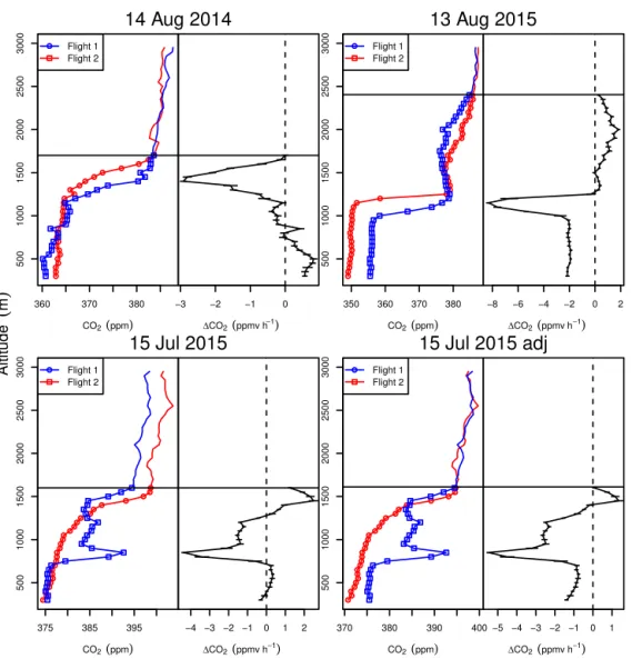
The observed vertical profiles of carbon dioxide and associ-ated NEE values (Fig. 4) often exhibited characteristics of the ideal flight (Fig. 1), but there was more variation and some flights exhibited more complexity. Many flights had a sharp decrease in carbon dioxide mixing ratios that corresponded to a well-defined boundary layer height. For example, the sec-ond flight on 14 August 2014 had a boundary layer height that increased by approximately 250 m compared to the first flight (Fig. 4, top-left panel). This is consistent with the growth in the boundary layer over a 3 h period (Stull, 1988, Fig. 1.7). Above around 1800 m, carbon dioxide mixing ra-tios between the two flights approximately matched, as ex-pected. For the flights on 13 August 2015, the carbon dioxide mixing ratios observed within the mixed layer showed near-ideal behavior (Fig. 4, top-right panel). In this case, both a de-crease in carbon dioxide mixing ratio within the mixed layer and an increase in the boundary layer height were observed. However, above the transition, there is a difference in mixing ratios that cannot be unequivocally assigned to local surface exchange. The calculated positive contribution to NEE from approximately 1500 to 2400 m could be attributed to entrain-ment processes and therefore would be considered as part of the surface exchange. The more complex structure of the profile observed during the first flight could be attributed to a residual mixed layer from the previous day. Alternatively, the increase in carbon dioxide mixing ratios could be due to long-range transport and changes in the source regions of the free-tropospheric winds. This would be a violation of our as-sumption of spatial homogeneity and should not be included in the surface NEE summation. Our current analysis includes this contribution, but additional information about boundary layer structure (for example, profiles of temperature and hu-midity) could resolve this question.
360 370 380 500 1000 1500 2000 2500 3000
CO2 (ppm)
● ● ●● ●● ● ●● ● ●● ● ●● ● ● ●● ● ●● ●● ● ● ●● ● ● Flight 1
Flight 2
∆CO2 (ppmv h−1)
14 Aug 2014
−3 −2 −1 0 350 360 370 380
500 1000 1500 2000 2500 3000
CO2 (ppm)
● ●● ●● ● ● ● ● ● ●● ● ● ●● ●● ● ● ● ● ● ● ●● ●● ●● ●● ●● ●● ●● ●● ●● ● ● Flight 1
Flight 2
∆CO2 (ppmvh−1)
13 Aug 2015
−8 −6 −4 −2 0 2
375 385 395
500 1000 1500 2000 2500 3000
CO2 (ppm)
●● ●● ●● ● ●● ●● ●● ●● ●● ●● ●● ●● ● ● ●● ● Flight 1
Flight 2
∆CO2 (ppmv h−1)
15 Jul 2015
−4 −3 −2 −1 0 1 2 370 380 390 400
500 1000 1500 2000 2500 3000
CO2 (ppm)
●● ●● ●● ● ●● ● ● ●● ●● ●● ●● ●● ●● ● ● ● ● ● Flight 1
Flight 2
∆CO2 (ppmv h−1)
15 Jul 2015 adj
−5 −4 −3 −2 −1 0 1
A lt it u d e
(
m)
Figure 4.The left portion of each panel shows the mixing ratio of carbon dioxide to an altitude of 3000 m for the two launches (blue for the first launch, red for the second). The differences in carbon dioxide mixing ratio contribute to the calculated NEE and also help to visualize
mixed-layer processes (1CO2). The error bars for1CO2are 1 standard error. The top-left panel from 14 August 2014 shows a flight that has
little change in the mixed-layer carbon dioxide mixing ratio, but the increase in boundary layer height leads to negative values for1CO2and
hence a negative NEE. The top-right panel from 13 August 2015 shows a flight that has both a decrease in mixed-layer carbon dioxide mixing
ratio and an increase in the boundary layer height, contributing to a negative NEE. However, there is also a positive1CO2above the mixed
layer that is not straightforward to interpret (see text). The bottom panels from 15 July 2015 demonstrate a flight that was corrected due to instrumentation error. The original data (bottom-left) had carbon dioxide mixing ratios that differed consistently in the free troposphere. This was corrected to match free-tropospheric carbon dioxide mixing ratios between flights and produced reasonable profiles of carbon dioxide
mixing ratio and1CO2in the boundary layer (bottom-right).
gain additional information about the boundary layer struc-ture from the water vapor profile. However, with this new instrument, carbon dioxide mixing ratios in the free tropo-sphere systematically differed between flights, unlike all the other flights where they were closely matched. Mixing ra-tios of carbon dioxide for the second flight were consistently 4 ppmv higher than the first flight, which is a factor of ap-proximately 1 % of the total mixing ratio. We speculate that there was an error with the internal pressure sensor of the LI-840. Given this empirical observation, the data were ad-justed by reducing both the recorded carbon dioxide mixing
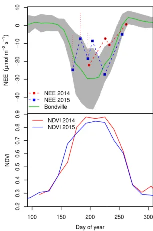
3.1 Comparison of HAB results with other data sources Our observations of NEE seasonal trends mostly matched our expectations derived from NDVI satellite values and a nearby EC site in Bondville, Illinois. In 2014, HAB NEE val-ues were most negative in mid July (−22.1 µmol m−2s−1) and became more positive as the summer went on (Fig. 5). In 2015, there was a minimum on 13 August 2015 (day of year 225) at −27.3 µmol m−2s−1 and a maximum on 9 September 2015 (day of year 255) of−5.0 µmol m−2s−1, and there was more variability compared to 2014. For 2014, there are only four HAB measurements and therefore only limited conclusions about the annual cycle can be drawn, but the timing of their minimum and maximum match within the 10-day averaging window of the EC values (Fig. 5). While the HAB maximum for 2015 is consistent with the EC trend, the HAB minimum occurs much later (day of year 255 vs. 205). Further research with more measurement dates is nec-essary to determine if the variability observed in 2015 was due to experimental imprecision or intrinsic variability in NEE. One possibility is that the sensor correction used for three flights in 2015 introduced experimental error that ob-scured the seasonal trend in HAB NEE. While the empirical correction produced free-tropospheric carbon dioxide mixing ratios that matched between the two flights, we do not under-stand the nature of the instrument malfunction and therefore we cannot assess its potential impact on the corrected NEE values.
An inspection of NDVI values (Fig. 5) does not reveal any obvious differences between 2014 and 2015 that would ac-count for increased variability in 2015. Lower NDVI values in 2015 could reflect increased plant stress, but this is spec-ulative. NDVI values reach their fall minimum later than the HAB NEE become positive (net respiration), but this is also true for the comparison with the long-term EC NEE values from Bondville. The timing of the fall decrease in our NDVI values is roughly consistent with seasonal NDVI trends from an agricultural area of Nebraska (Eastman et al., 2013). The lag between NEE and NDVI decreases could be due to the time that crops spend in the field before harvest. In late sum-mer and fall, crops do not have a positive net photosynthe-sis, but agricultural practice is to leave crops in place to dry out. NDVI might continue to sense vegetation when crops are present in the field even if they are not undergoing pho-tosynthesis due to senescence.
Our results are consistent in magnitude with smaller-scale measurements from the Bondville flux site. The other HAB NEE measurements are either within or very close to within 1 standard deviation of the long-term (13-year) mean of the EC data (Fig. 5). Finally, the overall seasonal trends from both 2014 and 2015 and the magnitude of the values are consis-tent with the trends and the range of observed data collected using the first-generation approach from 2012 to 2013 (Pocs, 2014).
N
E
E
(
µ
m
o
l
m
−
2s
−
1)
−40
−30
−20
−10
0
10
● ●
● ●
● NEE 2014
NEE 2015 Bondville
100 150 200 250 300
0.2
0.3
0.4
0.5
0.6
0.7
0.8
0.9
Day of year
ND
VI
NDVI 2014 NDVI 2015
Figure 5.Seasonal patterns in NDVI (bottom panel) and NEE (top panel) for 2014 and 2015 and data from the Bondville eddy flux site for 1996 to 2008. NEE data in the top panel include the NEE HAB estimates (dashed lines and filled circles (2014) and squares (2015)) and 10-day averages of midday (11:00–15:00 local standard time) NEE for Bondville (green solid line). The gray shaded region indi-cates 1 standard deviation above and below the mean for Bondville.
The vertical black lines are±1 standard error for the HAB NEE
esti-mates. The vertical red dotted lines show the instrument adjustment that was necessary for three of the flights. HAB-based NEE falls within or very close to the shaded region. NDVI generally tracks NEE well, but NEE from both Bondville and the HAB technique approaches zero sooner than NDVI in the fall.
3.2 Error analysis
dif-ferent measurements of carbon dioxide mixing ratio. Assum-ing that mixAssum-ing ratios should be constant within a 50 m bin, the standard error for the1CO2for each bin (also assuming
errors are not correlated) is given in Fig. 4 (right-side of each panel). Propagating these errors to the NEE estimate leads to the conclusion that random errors are not significant. Vi-sually, the standard errors are smaller than the plotting char-acters in Fig. 5 and all are less than 0.7 µmol m−2s−1. The statistical errors associated with assuming a constant poten-tial temperature are also small. Ther2value exceeded 0.999 for all of the linear fits. Systematic measurement error could potentially be much larger. Examining the first term on the right-hand side of Eq. (2), errors in estimating the mass of the column scale linearly. For example, a 1 % error in the pres-sure meapres-surement would translate into a roughly 1 % error in the column mass, which is small. In contrast, the calculation of surface exchange depends of the difference of the two av-eraged carbon dioxide mixing ratios. If there were an error of 1 % from one flight to the next, there would be a large error in the difference. That this error is relatively minimal is seen in the good match of the carbon dioxide mixing ratios above the mixed layer. For example, the match above 2500 m for 13 August 2015 (Fig. 4) is very good and is typical of most of the flights.
Another source of potential error is that the air measured by the carbon dioxide instrument was not dried. Since the mixing ratio output of the instrument depends on the mea-sured air pressure, a flux of water vapor into the bound-ary layer will lead to a bias. This error can be assessed by assuming a typical evapotranspiration flux of water vapor and using the boundary layer height of 1500 m from the 14 August 2014 flight (Fig. 4). This simple treatment ig-nores boundary layer growth and the entrainment of drier air from the free troposphere, so it is a upper bound on the error. Using a typical corn–soy crop evapotranspiration rate of 0.70 mm h−1 gives an integrated flux into the col-umn of 2.1 kg of water vapor over 3 h, the typical flight time. On 14 August 2014, the column mass was approximately 1500 kg, and accounting for the differences in the molecu-lar masses of air and water vapor gives a pressure impact of 0.23 %. Assuming the error in the carbon dioxide mix-ing ratio is linear with small changes in pressure and usmix-ing a mixing ratio of 365 ppmv and again the flight time of 3 h, the effect on1CO2would be approximately 0.28 ppmv h−1.
For this upper-bound error estimate, the effect would be 4 µmol m−2s−1 for the 14 August 2014 flight. This points
out the need to understand this effect more fully in future measurement campaigns and demonstrates our motivation to use an instrument that measures water vapor.
Horizontal advection is a potential source of error with the assumptions of the fixed-mass column approach. To consider errors associated with advection in the mixed layer, back tra-jectories were calculated for each flight day. Details are given in the Supplement, but due to the relatively short time be-tween flights (3 h), changes in the source regions were small.
Given the homogeneous landscape of the Midwestern corn– soy rotation, the potential error due to advection within the mixed layer is minimized. Laubach and Fritsch (2002) ex-amined the role of advection above the mixed layer using the subsidence velocity and mixing ratio profiles, and they found the contribution to be small in most cases. They judged the correction to be “often not worthwhile” but did note some ex-ceptions. As noted below, an advantage of the HAB method-ology is its low cost. This opens the possibility to use mul-tiple systems on the same day, which could be done along a wind transect to assess the role of horizontal advection in a quantitative way.
3.3 Advantages and limitations of the HAB methodology
The HAB methodology has numerous advantages. (1) It is a direct mass-balance approach. There are no assumptions necessary to calculate the surface exchange: the equations rely only on the ideal gas law. (2) Using a single instrument to measure both carbon dioxide vertical profiles reduces er-rors inherent in difference measurements. By comparing the two carbon dioxide profiles retrieved above the mixed layer, issues associated with sensor imprecision between flights can be assessed. This allowed us to spot problems with the LI-840 instrument compared to the more stable LI-820. (3) The HAB methodology measures NEE at an intermediate scale between stationary eddy flux sites and regional-scale measurements derived from satellite inversions of remotely sensed carbon dioxide concentrations. (4) The costs associ-ated with HAB are modest compared to aircraft flux mea-surements. This lowers the barrier for entry and opens the possibility for citizen science groups to contribute measure-ments. For example, high school students have observed and assisted our launches.
There are some drawbacks. Most importantly, conduct-ing balloon launches is time intensive and measurements are episodic. Unlike the continuous half-hour data stream from an EC tower, measurements need to be acquired by hand. Because of this, the method is useful for temporally lim-ited comparisons to other data sources as done in the current study, but they would increase is not appropriate for calculat-ing annual net NEE values by itself.
between flights (4 h maximum) and the same wind speed to get a distance of 64 km. A more detailed study of turbulent mixing would be necessary to assess the footprint extent per-pendicular to the horizontal wind direction. The necessity for a spatially homogeneous landscape limits the locations for deployment. Even if this condition is met, forested land-scapes, urban areas and private property pose an issue for in-strument retrieval. A tethered balloon system would address this problem, but increase the complexity of the experiment.
4 Conclusions
Further research with the HAB methodology could be done to extend the validity of the method. Multiple launches could be conducted on the same day in different locations, which would help assess the spatial footprint of the HAB method-ology. A series of more than two launches performed on one day at the same location would allow diurnal cycles in NEE to be considered. Both of these improvements require mul-tiple launch teams, which could be used as an opportunity to recruit citizen scientists into the process. The AirCore ap-proach (Karion et al., 2010) will also be considered, since multiple citizen scientist teams could use this low-cost sam-pling method, with analysis taking place at a central labora-tory. The launch site could be moved to a more agricultural landscape, which could minimize the influence of local an-thropogenic sources potentially in Pontiac. The methodology would also provide useful information for regional-scale in-version estimates (Gourdji et al., 2012) that could account for the advective component of the observed carbon dioxide profiles.
Because of the massive human perturbation of the natu-ral carbon cycle due to agriculture, landscape-scale measure-ments are necessary to understand the fully integrated sur-face exchanges. While small-scale eddy flux measurements are a good tool for assessing particular agricultural practices at the plot scale, the HAB methodology can be used to ver-ify carbon dioxide exchanges over much larger spatial scales. Agriculture occupies a vast amount of land, so understanding its ability to take up or release carbon dioxide is crucial for understanding the global carbon cycle as a whole.
5 Data availability
For this initial exploration of the HAB methodology, the datasets are available upon request from the corresponding author. In the future, all data generated by citizen scientists will be open access.
Three external sources of data were used in this analy-sis. Vertical velocities were derived from the NCEP reanaly-sis (http://www.esrl.noaa.gov/psd/cgi-bin/data/narr/plothour. pl) (NOAA, 2016a). The NDVI values from MODIS came from the Reverb/ECHO tool (http://reverb.echo.nasa.gov/) (NASA, 2016). The EC flux data were from the Ameriflux
network server (http://ameriflux.lbl.gov/data/download-data/ ?site_id=US-Bo1) (AmeriFlux, 2016). In addition, NOAA reanalysis data were used for the trajectories calculated in the Supplement (ftp://arlftp.arlhq.noaa.gov/pub/archives) (NOAA, 2016b).
The Supplement related to this article is available online at doi:10.5194/amt-9-5707-2016-supplement.
Acknowledgements. We thank Paul Ritter and Eric Bohm of Pontiac Township High School for access to the launch site. We appreciate the students that have given assistance on launches, including Cody Sabo, Mary Babiez, David Wilson, Becky Dietrich, Mike Cole and students from Harold Washington College’s High Altitude Ballooning research team. We would also like to thank the Illinois Space Grant Consortium/NASA for providing funding for this project.
Edited by: T. Wagner
Reviewed by: two anonymous referees
References
AmeriFlux: AmeriFlux data, available at: http://ameriflux.lbl.gov/ data/download-data/?site_id=US-Bo1, last access: 28 Novem-ber 2016.
Baldocchi, D., Falge, E., Gu, L., Olson, R., Hollinger, D., Run-ning, S., Anthoni, P., Bernhofer, C., Davis, K., Evans, R., Fuentes, J., Goldstein, A., Katul, G., Law, B., Lee, X., Malhi, Y., Meyers, T., Munger, W., Oechel, W., Paw, K. T., Pile-gaard, K., Schmid, H. P., Valentini, R., Verma, S., Vesala, T., Wilson, K., and Wofsy, S.: FLUXNET: a new tool to study the temporal and spatial variability of ecosystem-scale carbon dioxide, water vapor, and energy flux densi-ties, B. Am. Meteorol. Soc., 82, 2415–2434, doi:10.1175/1520-0477(2001)082<2415:FANTTS>2.3.CO;2, 2001.
Barcza, Z., Kern, A., Haszpra, L., and Kljun, N.: Spatial represen-tativeness of tall tower eddy covariance measurements using re-mote sensing and footprint analysis, Agr. Forest Meteorol., 149, 795–807, doi:10.1016/j.agrformet.2008.10.021, 2009.
Chou, W. W., Wofsy, S. C., Harriss, R. C., Lin, J. C., Gerbig, C.,
and Sachse, G. W.: Net fluxes of CO2in Amazonia derived from
aircraft observations, J. Geophys. Res.-Atmos., 107, ACH 4–1– ACH 4–15, 4614, doi:10.1029/2001JD001295, 2002.
Churkina, G., Schimel, D., Braswell, B. H., and Xiao, X.: Spatial analysis of growing season length control over net ecosystem ex-change, Glob. Change Biol., 11, 1777–1787, doi:10.1111/j.1365-2486.2005.001012.x, 2005.
Denmead, O., Raupach, M., Dunin, F., Cleugh, H., and Leun-ing, R.: Boundary layer budgets for regional estimates of scalar fluxes, Glob. Change Biol., 2, 255–264, doi:10.1111/j.1365-2486.1996.tb00077.x, 1996.
Eastman, J. R., Sangermano, F., Machado, E. A., Rogan, J., and Anyamba, A.: Global trends in seasonality of normalized differ-ence vegetation index (NDVI), 1982–2011, Remote Sensing, 5, 4799, doi:10.3390/rs5104799, 2013.
Enting, I. G., Trudinger, C. M., and Francey, R. J.: A synthesis
inver-sion of the concentration andδ13C of atmospheric CO2, Tellus
B, 47, 35–52, doi:10.1034/j.1600-0889.47.issue1.5.x, 1995. Gourdji, S. M., Mueller, K. L., Yadav, V., Huntzinger, D.
N., Andrews, A. E., Trudeau, M., Petron, G., Nehrkorn, T., Eluszkiewicz, J., Henderson, J., Wen, D., Lin, J., Fischer, M.,
Sweeney, C., and Michalak, A. M.: North American CO2
ex-change: inter-comparison of modeled estimates with results from a fine-scale atmospheric inversion, Biogeosciences, 9, 457–475, doi:10.5194/bg-9-457-2012, 2012.
Guan, K., Berry, J. A., Zhang, Y., Joiner, J., Guanter, L., Badg-ley, G., and Lobell, D. B.: Improving the monitoring of crop productivity using spaceborne solar-induced fluorescence, Glob. Change Biol., 22, 716–726, doi:10.1111/gcb.13136, 2016. Gurney, K. R., Law, R. M., Denning, A. S., Rayner, P. J., Baker, D.,
Bousquet, P., Bruhwiler, L., Chen, Y.-H., Ciais, P., Fan, S., Fung, I. Y., Gloor, M., Heimann, M., Higuchi, K., John, J., Maki, T., Maksyutov, S., Masarie, K., Peylin, P., Prather, M., Pak, B. C., Randerson, J., Sarmiento, J., Taguchi, S., Takahashi, T., and
Yuen, C.-W.: Towards robust regional estimates of CO2sources
and sinks using atmospheric transport models, Nature, 415, 626– 630, doi:10.1038/415626a, 2002.
Gurney, K. R., Law, R. M., Denning, A. S., Rayner, P. J., Pak, B. C., Baker, D., Bousquet, P., Bruhwiler, L., Chen, Y.-H., Ciais, P., Fung, I. Y., Heimann, M., John, J., Maki, T., Maksyutov, S., Peylin, P., Prather, M., and Taguchi, S.: Transcom 3 inversion in-tercomparison: Model mean results for the estimation of seasonal carbon sources and sinks, Global Biogeochem. Cy., 18, gB1010, doi:10.1029/2003GB002111, 2004.
Hollinger, S. E., Bernacchi, C. J., and Meyers, T. P.: Car-bon budget of mature no-till ecosystem in North Central Re-gion of the United States, Agr. Forest Meteorol., 130, 59–69, doi:10.1016/j.agrformet.2005.01.005, 2005.
Horst, T. W. and Weil, J. C.: Footprint estimation for scalar flux measurements in the atmospheric surface layer, Bound.-Lay. Me-teorol., 59, 279–296, doi:10.1007/BF00119817, 1992.
Karion, A., Sweeney, C., Tans, P., and Newberger, T.: AirCore: An innovative atmospheric sampling system, J. Atmos. Ocean. Tech., 27, 1839–1853, doi:10.1175/2010JTECHA1448.1, 2010. Krausmann, F., Erb, K.-H., Gingrich, S., Haberl, H., Bondeau,
A., Gaube, V., Lauk, C., Plutzar, C., and Searchinger, T. D.: Global human appropriation of net primary production doubled in the 20th century, P. Natl. Acad. Sci. USA, 110, 10324–10329, doi:10.1073/pnas.1211349110, 2013.
Laubach, J. and Fritsch, H.: Convective boundary layer budgets de-rived from aircraft data, Agr. Forest Meteorol., 111, 237–263, doi:10.1016/S0168-1923(02)00038-2, 2002.
Luo, Z., Wang, E., and Sun, O. J.: Can no-tillage stimulate carbon sequestration in agricultural soils? A meta-analysis of paired experiments, Agr. Ecosyst. Environ., 139, 224–231, doi:10.1016/j.agee.2010.08.006, 2010.
Martins, K. D., Sweeney, C., Stirm, B. H., and Shepson, P. B.:
Re-gional surface flux of CO2inferred from changes in the advected
CO2 column density, Agr. Forest Meteorol., 149, 1674–1685,
doi:10.1016/j.agrformet.2009.05.005, 2009.
Mays, K. L., Shepson, P. B., Stirm, B. H., Karion, A., Sweeney, C., and Gurney, K. R.: Aircraft-based measurements of the carbon footprint of Indianapolis, Environ. Sci. Technol., 43, 7816–7823, doi:10.1021/es901326b, 2009.
Meyers, T. P. and Hollinger, S. E.: An assessment of storage terms in the surface energy balance of maize and soybean, Agr. Forest Meteorol., 125, 105–115, doi:10.1016/j.agrformet.2004.03.001, 2004.
Mkhabela, M. S., Mkhabela, M. S., and Mashinini, N. N.: Early maize yield forecasting in the four agro-ecological
regions of Swaziland using NDVI data derived from
NOAA’s-AVHRR, Agr. Forest Meteorol., 129, 1–9,
doi:10.1016/j.agrformet.2004.12.006, 2005.
Monson, R. and Baldocchi, D.: Terrestrial Biosphere-Atmosphere Fluxes, Cambridge University Press, ISBN-13: 978-1-107-04065-6, Cambridge, UK, 2014.
NASA: MODIS data, available at: http://reverb.echo.nasa.gov/, last access: 28 November 2016.
NOAA: NCEP data, available at: http://www.esrl.noaa.gov/psd/ cgi-bin/data/narr/plothour.pl, last access: 28 November 2016a. NOAA: NCEP/NCAR Reanalysis data, available at: ftp://arlftp.
arlhq.noaa.gov/pub/archives/, last access: 28 November 2016b. Peters, W., Jacobson, A. R., Sweeney, C., Andrews, A. E.,
Con-way, T. J., Masarie, K., Miller, J. B., Bruhwiler, L. M. P., Petron, G., Hirsch, A. I., Worthy, D. E. J., van der Werf, G. R., Ran-derson, J. T., Wennberg, P. O., Krol, M. C., and Tans, P. P.: An atmospheric perspective on North American carbon dioxide ex-change: CarbonTracker, P. Natl. Acad. Sci. USA, 104, 18925– 18930, doi:10.1073/pnas.0708986104, 2007.
Pocs, M.: A high-altitude balloon platform for exploring the terrestrial carbon cycle, DePaul Discoveries, 3, Article 2, http://via.library.depaul.edu/depaul-disc/vol3/iss1/2/ (last ac-cess: 14 November 2016), 2014.
Poeplau, C. and Don, A.: Carbon sequestration in agricultural soils via cultivation of cover crops – A meta-analysis, Agr. Ecosyst. Environ., 200, 33–41, doi:10.1016/j.agee.2014.10.024, 2015. Potosnak, M. J., Wofsy, S. C., Denning, A. S., Conway, T. J.,
Munger, J. W., and Barnes, D. H.: Influence of biotic
ex-change and combustion sources on atmospheric CO2
con-centrations in New England from observations at a for-est flux tower, J. Geophys. Res.-Atmos., 104, 9561–9569, doi:10.1029/1999JD900102, 1999.
Potter, C., Klooster, S., Huete, A., and Genovese, V.: Terrestrial car-bon sinks for the United States predicted from MODIS satel-lite data and ecosystem modeling, Earth Interact., 11, 1–21, doi:10.1175/EI228.1, 2007.
R Core Team: R: A Language and Environment for Statistical Com-puting, R Foundation for Statistical ComCom-puting, Vienna, Austria, https://www.R-project.org/, last access: 14 November 2016. Reuter, M., Buchwitz, M., Hilker, M., Heymann, J., Schneising, O.,
Atmos. Chem. Phys., 14, 13739–13753, doi:10.5194/acp-14-13739-2014, 2014.
Schneising, O., Heymann, J., Buchwitz, M., Reuter, M., Bovens-mann, H., and Burrows, J. P.: Anthropogenic carbon dioxide source areas observed from space: assessment of regional en-hancements and trends, Atmos. Chem. Phys., 13, 2445–2454, doi:10.5194/acp-13-2445-2013, 2013.
Sims, D. A., Rahman, A. F., Cordova, V. D., El-Masri, B. Z., Baldocchi, D. D., Bolstad, P. V., Flanagan, L. B., Goldstein, A. H., Hollinger, D. Y., Misson, L., Monson, R. K., Oechel, W. C., Schmid, H. P., Wofsy, S. C., and Xu, L.: A new model of gross primary productivity for North American ecosystems based solely on the enhanced vegetation index and land surface temperature from MODIS, Remote Sens. Environ., 112, 1633– 1646, doi:10.1016/j.rse.2007.08.004, 2008.
Stull, R.: An Introduction to Boundary Layer Meteorology, At-mospheric Science Library, Springer, ISBN-10: 90-277-2769-4, Dordrecht, the Netherlands, 1988.
Sus, O., Heuer, M. W., Meyers, T. P., and Williams, M.: A data as-similation framework for constraining upscaled cropland carbon flux seasonality and biometry with MODIS, Biogeosciences, 10, 2451–2466, doi:10.5194/bg-10-2451-2013, 2013.
West, T. O., Brandt, C. C., Baskaran, L. M., Hellwinckel, C. M., Mueller, R., Bernacchi, C. J., Bandaru, V., Yang, B., Wilson, B. S., Marland, G., Nelson, R. G., Ugarte, D. G. D. L. T., and Post, W. M.: Cropland carbon fluxes in the United States: increasing geospatial resolution of inventory-based carbon ac-counting, Ecol. Appl., 20, 1074–1086, doi:10.1890/08-2352.1, 2010.