B RUNOH OPP, GESIS Leibniz Institute for the Social Sciences, Cologne

Strategies in Computer-Assisted Text Analysis

Revised

19th July 2016

ALAN BRIER, ESRC National Centre for Research Methods, University of Southampton

ELISABETTA DE GIORGI, Portuguese Institute of International relations (IPRI), NOVA University of Lisbon

BRUNO HOPP, GESIS Leibniz Institute for the Social Sciences, Cologne

This paper reviews the logic of attempts to automate the processes involved in computer-assisted text analysis in the social sciences. Bayesian estimation methods in spatial analysis of variations in positions of political parties over time and Latent Dirichlet Allocation from the developing field of latent topic analysis are compared with the analysis of structures of word co-occurrences in the tradition of content analysis, using Procrustean

Introduction

There is a welcome revival of interest in systematic analysis of the rich resources of textual data increasingly available, not least marked by a special issue of Political Analysis, the journal of the Society for Political Methodology and the Political Methodology Section of the American Political Science Association (Monroe, Schrott, 2008). Interest in analysing elements of discourse is nothing new, but since the early days of computer-assisted content analysis, it has often been left to qualitative methods of investigation alone by the majority of the social sciences. There is no reason why it should not be accorded a place in the general repertoire of methods of statistical inference in common use. In this article we hope to clarify the issues raised by comparing two broad approaches, prompted in part by Bara, Weale and Bicquelet (2007) (BWB), who compared an earlier version of our HAMLET II software (Brier, Hopp 2011) with Alceste (Reinert 2005), calling the former “semi-automated” and the latter “fully

automated”. Since they reported their experience in applying these to parliamentary debates,

we will also illustrate the contrasted research strategies with reference to the opening debate on the Italian budget of 1997 (L. 663/96 Legge finanziaria, 1997).

Until recently, the question of the general method to use appeared to have been settled in favour of essentially dictionary-based searching for terms of analytical interest, individually and occurring together in characteristic patterns. With particular reference to Woelfel’s CATPAC II software, based on the automatic extraction of collocations, Juliane Landmann and Cornelia Züll (2004) argued convincingly that it was not advisable to dispense completely with some kind of a priori dictionary for this purpose. To do so could involve serious risks of misinterpretation resulting from misleading representation of relationships between words and expressions in the texts to be considered, Depending on the richness of the language to be analysed, this could consist of single words, with or without lemmatization, or an elaborated set of categories, each defined by sets of words to be attributed to them, and not necessarily mutually exclusive. The Identity Project at Harvard’s Weatherhead Center for International Affairs (2002) has left a collection of dictionaries used by researchers including Laver and Garry (2000), together with the Yoshikoder (http://www.yoshikoder.org/resources.html), a cross-platform multilingual content analysis GPL Java program developed for their production for use with various text corpora.

The logic of seeking to dispense with a “dictionary” of this nature is apparent in the approaches adopted in TextAnalyst (Microsystems Limited 2001) and Leximancer (Smith, Humphreys 2006). In each case, however, identification of co-occurrences proceeds after ignoring a list of words specified in advance as unlikely to contribute significantly to the analytical content of the material to be read. “Stoplists” of this kind are usually present by default for the language of the target text, and may additionally be “trained” to take account of particular kinds of discourse, before being applied to the selection of candidate words for consideration. Our experience in working with texts of various kinds from differing sources is that it is not possible to extract meaningful associations of word usage without BOTH ignoring words to be considered as 'trivial' AND specifically including words of particular theoretical relevance to the intended analysis.

or, for that matter, the process of dictionary construction.1 _{WordStat from Provalis Research} now offers a Naïve Bayesian machine learning algorithm in addition to a K-Nearest Neighbours technique (KNN) for document classification.

Some interesting innovations in techniques have emerged in the field of spatial analysis of variations over time in the positions expressed in manifestos of political parties. Wordscores (Benoit and Laver 2003; Laver et al. 2003) was a pioneering method of automated content analysis that assigns policy positions or ‘‘scores’’ to documents on the basis of word counts by relating them to word distributions from reference texts considered to represent extreme points of the political space. The method is straightforward to implement, requires no functional or distributional assumptions, and has been found to work well in many applications. But Lowe(2008) has shown that it can be expected to produce non-biased estimates only if the conditions are met for it to approximate the maximum likelihood equations for an ideal point model equivalent to a single dimensional correspondence analysis of the document-word matrix. However, in treating all words as equally informative, Wordscores has no way to distinguish politically uninformative from centrist words or discount words that occur more frequently than others for linguistic rather than political reasons. Natural language text exhibits highly skewed word frequency distributions (Zipf 1949, p.22-27) and inevitably contains many uninformative words. A problem of bias due to insufficient overlap of word distributions between reference documents or inappropriate distributions of wordscores is of less importance in practice, but two final conditions cannot simultaneously be met for any finite data set, so that “bias in wordscores, documents scores, or both is inevitable if correspondence analysis or wordscores is used as an estimator. …. If the parameters of the [implicit model] are estimated directly, for example by maximum likelihood or inferred using Bayesian methods rather than via the correspondence analysis or Wordscores approximations, then these biases should disappear.” (Lowe, 2008, p.369)

The Wordfish algorithm proposed by Proksch and Slapin (2008, 2009) seems to provide confirmation of this expectation. It also begins with term document matrices, this timebased on a series of separate text corpora for different policy areas to produce more concentrated word distributions across each set of texts. The cells of a matrix contain the number of times each unique word is mentioned in each document. The word frequencies in the documents are assumed to generated by a simple Poisson process, also used by Monroe and Maeda (2004), and an iterative Expectation-Maximization process is applied to estimate a model consisting of four parameters : document (party) positions on a single dimension, document (party) fixed effects, word weights (discriminating parameters), and word fixed effects (due to their linguistic functions):

where yijt is the frequency of word j in the manifesto of party i at time t, α is a vector of party-election year fixed effects, ψ is a vector of word fixed effects, β is an estimate of a word-specific weight capturing the importance of word j in discriminating between party positions and ω is the estimate of party i ‘s position in election t. (2008, p.709) Starting values for word and party fixed effects are based on the overall word frequencies and those of the manifestos in the first election considered. The left- and right-singular vectors from a singular value decomposition of the matrix of logged word frequencies, after subtracting the word and party fixed effects, are used as the starting values for the word weights (β) and party positions (ω).

Estimation involves first holding the party parameters fixed at a certain value while word parameters are estimated, then holding word parameters fixed at their new values while the party positions are estimated. This process is repeated until the parameter estimates reach an

acceptable level of convergence. The authors interpret the single dimension of discrimination as left versus right and obtain values for German parties over a series of elections from 1990 to 2005. They also offer a striking graphic relating word weights and word fixed effects which takes the shape of an “Eiffel Tower of words.” Words with a high fixed effect have zero weight, but words with low fixed effects have either negative or positive weight.

Words with large weights are observed to be those with a politically relevant connotation. (Slapin and Proksch, 2008, Fig.2, p.715).

Latent Dirichlet Allocation

A development of work in the tradition of latent topic analysis, Latent Dirichlet Allocation (LDA) (Blei et al., 2003) offers an elegant method of more general application than the single dimensional scaling of party manifestos which has been briefly reviewed above. It is concerned with the classification of pieces of text for purposes of indexing and retrieval according to the latent topics which they are supposed to contain. In the absence of any prior knowledge of the content of a series of texts, it has the possible advantage of producing a classification, in an extreme case, without requiring that they have any significant terms at all in common. The topics allocated need not necessarily be open to interpretation in themselves, as long as the text sources are reliably classifiable by their application.

A Bayesian estimation procedure applies a simple generation model to a number of texts or to the assembly of sentences or other context units specified within a single text. This assumes that each word occurring in a document is generated first by sampling a topic from a set of topic distributions, then choosing a word from the distribution of words in the topic in question. Steyvers and Griffiths (2007) offer a highly accessible account of this approach for the general reader.

The model specifies the following distribution over words within a document, where T is the number of topics:

Using φ(j) _{to refer to the multinomial distribution over words for topic j and} θ (d) _{the multinomial} distribution over topics for document d, these indicate respectively, which words are important for each topic and which topics are important for a particular document. Blei, Ng and Jordan (2003) proposed introducing a Dirichlet prior on θ, calling the result Latent Dirichlet Allocation.

The probability density of a T-dimensional Dirichlet distribution,

depends on an array of hyper-parameters (α1 .... αT), which, they suggest, can be understood as a kind of prior observation count, or pseudocounts, not necessarily integers, for the number of times topic j is sampled in a document before having observed any actual words from that document. The result is a smoothed topic distribution with the amount of smoothing determined by the α parameter.

assigned different values. It is after all only a matter of convenience to apply a symmetric Dirichlet prior with one uniform alpha parameter, determining the amount of smoothing of the topic distribution. Setting alpha < 1.0 disposes the process to topic distributions favouring only a few topics – creating a bias towards sparsity.

For computational convenience a Gibbs sampling procedure is commonly applied, which considers each word token in turn in a text corpus, which has usually first been subjected to various kinds of pre-processing (Feinerer et al. (2008), Grün and Hornik (2010)), and estimates the probability of assigning it to each topic, conditional on the topic assignments to all other word tokens. From this conditional distribution, a topic is sampled and stored as a new topic assignment for this word token, according to the following approximation (from Griffiths and Steyvers, 2004):

where CWT _{and C}DT _{are matrices consisting of the numbers of words by texts and documents} by texts respectively. In the expression shown, the left side is the probability of word w under topic j and the right side is the probability that topic j has under the current topic distribution for document d. Words therefore come to be assigned to topics depending upon how likely a word is for a topic, as well as how dominant a topic is in a document.

All word tokens contained in the text corpus are first randomly assigned to one of T topics, where T has to be specified in advance. Each Gibbs sample consists of the set of topic assignments to all N word tokens in the corpus, achieved by a single pass through all documents. For each word token, the count matrices CWT _{and C}DT _{are first decremented by} one for the entries that correspond to its current topic assignment. Then, a new topic is sampled from the distribution shown above and the count matrices CWT _{and C}DT _are incremented with the new topic assignment. After an initial “burn-in” period the successive Gibbs samples begin to approximate to the posterior distribution over topic assignments. To obtain a representative set of samples from this distribution, a number of Gibbs samples should be saved at regularly spaced intervals, to prevent correlations between samples (see Gilks et al. 1996).

These processes are seldom absolutely convergent, in the sense of two successive allocations being completely identical, but tend to settle down fairly rapidly to the same topic content at the higher expectation levels, with only slight variations in the numerical values.

Estimates φ’ and θ’ of the word-topic distributions and topic-document distributions can be obtained from the count matrices as follows:

These values correspond to the predictive distributions of sampling a new token of word i from topic j and of sampling a new token in document d from topic j. They are also the posterior means of these quantities conditional on a particular sample z.

This introduces a further set of initial assumptions which have to be made in any particular investigation. A standard list of the most common functional words in the relevant language can provide a starting point, and it is common also to disregard words which occur only a limited number of times in the material to be classified. It is clear, however, that in certain circumstances this will result in missing characteristic usages of certain texts or forms of expression. These can then no longer contribute to classification or interpretation of content in a meaningful way, both within individual documents or when attempting to compare a number of different documents.

If all of these largely a priori assumptions are to receive adequate consideration, it is unrealistic to expect Bayesian approaches of this kind to reduce very much the effort required on the part of the researcher in reaching a stable set of results, when compared with the traditional process of trying to define a dictionary-like search instrument on the basis of theoretical considerations. Repeated applications of LDA can, however, help to draw attention to the most frequent word tokens which, on consideration, would best be submitted in advance to lemmatization or stemming, take account of polymorphisms which may need to be interpreted as equivalent, and even assist in identifying significant synonyms, where these are allocated to the same topic. It is important to notice that topics in LDA are not in principle lists of co-occurrences. The individual words allocated to a particular topic have generally not been found to occur together within a relatively short span of words.

Although the methods described are often considered appropriate only for relatively large collections of documents, involving potentially exhaustive numbers of allocated topics, the compromises required in applying them to smaller-scale analyses using comparatively restricted computing resources do not necessarily prohibit the achievement of intelligible results. Nevertheless, it is clearly strongly advisable to test the effect of varying the arbitrary number of latent topics to be inferred, for α in addition to the other parameters already discussed, as this is the only way to be reasonably certain that a stable solution is available for given text corpus. It is quite possible, in our experience, that allocation to an excessive number of topics will be found to be numerically intractable, forcing a lower number to be applied. The topics themselves are also seldom likely to be open to sensible interpretation and are best regarded simply as a means of detecting the most effective word tokens to apply in comparing the various documents. Several researchers have noted that their results were not much affected by concentrating attention on only the words with the highest expectation values allocated to a specified number of topics when submitting the resulting table of documents by word tokens to further analysis, typically by methods involving singular value decomposition (SVD).2

An illustration

The issues involved can best be illustrated with an example, taken from a transitional period in the dramatic realignment in modern Italian politics which began in the early 1990s. “The implosion of the centre parties coincided with the end of the double exclusion of the communist left and the extreme right. Suddenly all of the parties gained a reasonable expectation to win access to government. In the new political landscape a bipolar competition developed between two broad alliances of the left and right respectively” (Verzichelli, Cotta, 2000: 243).

The 1994 election was won by the centre-right, composed of Forza Italia, Alleanza Nazionale and the Northern League, but the new government led by Silvio Berlusconi lasted just seven

2 An application to abstracts of 348 articles in the Journal of Statistical Software found varying

months because of the extreme heterogeneity of the alliance, and a technical government followed until the 1996 election. This was won by a centre-left coalition, composed of the Democratic Party of the Left (former PCI members who agreed with the party transformation of the early 1990s) and the Italian Popular Party (one of the Christian Democrat parties resulting from the split of the former DC), which had formed a new alliance called the Olive Tree with some other minor centre parties. Romano Prodi, the leader of the alliance, became Prime Minister in 1996, with the support of the Refounded Communist Party (the second, smaller party after the division of the former PCI) until 1998, when the latter refused a vote of confidence, leading to the government resignation.

For the purposes of this illustration, we apply a stoplist which suppresses all except those word tokens which are also admitted in the original dictionary-based analysis by Elisabetta De Giorgi (2008), based on the series of parliamentary debates identified in Table 2. This identifies a total of 346 words from the text corpus of over 13,000 words, of which 80 are unique tokens. These are initially randomly assigned to one of 8 topics. Adopting the uniform Dirichlet priors suggested by Steyvers and Griffiths (2007) (alpha=50/T = 6.25; beta = 0.01 for 2 <= T <= 10), after 601 iterations of the Gibbs sampler allocation process, with 87 % convergence. The top 50 tokens have been retained here for further analysis.

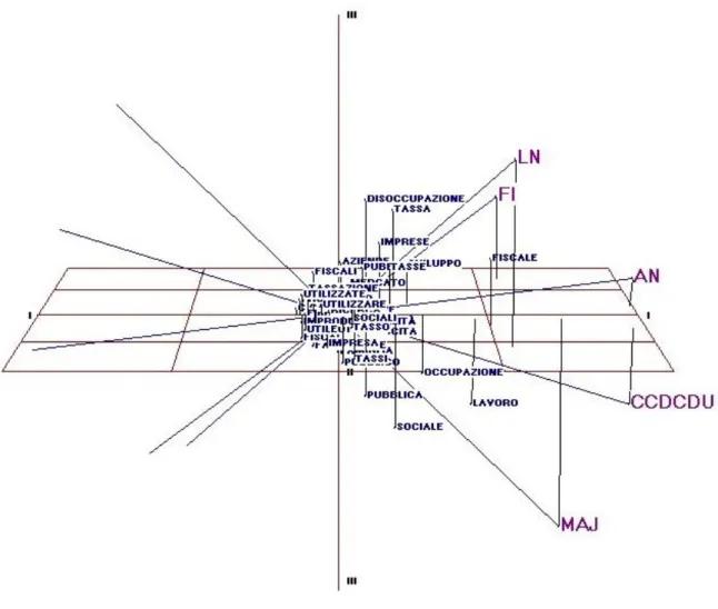
The topics allocated are shown in Table 1. The matrix of frequencies of these words by the documents considered can be visualised as shown in the biplot (Gower, Hand, 1996) reproduced in Figure 1.

The procedure applied here is adapted from MDPREF (Multidimensional Preferences Scaling)3_{, originally written by JD Carroll and JJ Chang(1969) to represent the strengths of} preferences of a number of subjects for the same group of stimuli but subsequently applied to values expressed as numerical scores. The document profiles are first normalised to unit length, to take account of differences in the document sizes, which enables them to be plotted as vectors of equal length through the configuration of points representing the word tokens

The next step finds the basic structure of the matrix A, consisting of the cross-products of the normalised profiles, by singular value decomposition, producing summary row and column vectors ( U and V) and a diagonal matrix of singular values d corresponding to the columns of A, so that

A = Ud(V/₎

The matrices U and V are the eigenvectors (principal components) of the matrices of row and column cross-products of A, and the d values are related to their (identical) eigenvalues (d=sqrt(D*(n-1)), where D is the diagonal of eigenvalues and n is the number of rows in A).4 Table 1 – Eight Topics resulting from Latent Dirichlet Allocation process

Topic 1

SVILUPPO 0.330 TASSA 0.264 PUBBLICO 0.176 FISCALI 0.088 POVERI 0.044

Topic 5

FISCALE 0.573 TASSO 0.110 BANCA 0.066 UTILIZZARE 0.044 CRESCITA 0.022

3 For further discussion of this procedure see Weller and Romney (1990) and Borg and

Groenen (2005), pp340 ff. Figure 1 shows the decomposition in three dimensions. Pearson correlation of the first and second score matrices = 0.886.

4 The first paper containing a fully worked-out numerical example corresponding to current

FISCO 0.022 LAVORO 0.022 TASSAZIONI 0.022

EGUALMENTE 0.022 FAMIGLIE 0.022

Topic 2

DISOCCUPAZIONE 0.396 AZIENDE 0.242 MERCATI 0.176 LAVORI 0.044 PRODURRÀ 0.044 UTILIZZATE 0.044 CAPITALE 0.022 CAPITALIZZARE 0.022

Topic 6

OCCUPAZIONE 0.264 SOCIALE 0.242 FAMIGLIA 0.088 CAPITALI 0.066 IMPRESA 0.066 TASSAZIONE 0.044 UTILE 0.044

Topic 3

TASSE 0.286 PUBBLICI 0.242 TASSI 0.176 IMPRENDITORIALI 0.022 INDUSTRIALI 0.022

Topic 7

LAVORO 0.462 CRESCITA 0.154 FAMIGLIE 0.066 FAMILIARE 0.044 FAMILIARI 0.044 PENSIONI 0.044 PRODURRE 0.044

Topic 4

IMPRESE 0.352 MERCATO 0.220 RICERCA 0.110 OPPORTUNITÀ 0.066 BANCO 0.044 PRODUTTIVA 0.044 FISCAL 0.022

Topic 8

PUBBLICA 0.220 SOCIALI 0.220 PRODUTTIVE 0.088 PRODUTTIVI 0.066 PRODUZIONI 0.066 FISCALITÀ 0.044 IMPRENDITORI 0.044

Note that it is possible for tokens to be allocated to more than one topic, as is here the case with CRESCITA, LAVORO and FAMIGLIE

MDPREF is a linear (or metric) procedure and the measure of goodness-of-fit of the model to the data is a product-moment correlation. If we consider one document vector passing through a configuration of stimulus points with perpendicular lines projected from the points onto the vector, it is the values given to the points at which these perpendicular lines meet the vector which are maximally correlated with that document's data. This vector indicates the direction in which the emphasis on a particular constellation of word usage increases over the word space. Substantively this makes a strong assumption about the nature of preference, in that the model implies an "ideal" point at infinity (which is similar to the classic econometric assumption of insatiability)5_{. In MDPREF, where the point of maximum preference is at infinity,} the contours are perpendicular to the vector. The document vectors are normalised (for convenience only) to unit length, so that their ends lie at a common distance from the origin of the space, forming a circle, or sphere, according to the number of dimensions plotted.

This avoids the difficulties of interpretation which can arise with naïve use of the related procedure of correspondence analysis, which is commonly offered in contexts of this kind. In Alceste, and in some more recent commercial software (e.g. Provalis Research QDA Miner; Lewis, Maas, 2007) results are visualised using methods derived from correspondence analysis (Greenacre, 1993; Weller, Romney, 1990), which, at least when used in isolation, involve a significant risk of erroneous interpretation of the results6

5 The objection to applying an ‘ideal point’ scaling in Wordscores (Lowe, 2008) appears to be met in this case : the matrix employed does not consist of raw document word frequencies but has been produced by LDA, including the effects of implied pre-processing of the original documents.

6 . If correspondence analysis is applied to the matrices of documents by words and topics

Figure 1 Singular Value Decomposition of matrix of documents by words7

.

matrix, but first transforms it by dividing each row entry by the square root of the product of the corresponding row and column totals, their geometric mean, removing differences in the marginal totals and expressing each cell as a proportion. If any of these products is zero, which is not improbable when comparing word frequencies in documents, the corresponding row and column entries have to be ignored in subsequent analysis. In addition, the results of correspondence analysis are often represented visually in the form of joint plots of the row and column points although these are strictly incommensurate, so that interpretation of inter-set pairs of points in terms of Euclidean distance, except in cases where the profiles compared vary substantially and are strongly unimodal, is likely to be seriously misleading. (Greenacre,

problem if we wish to associate documents with particular words or groups of words, and would

require convincing interpretation of the topics.

7 The party groups are: AN – Alleanza Nazionale (National Alliance); CCD – Centro Cristiano

Democratico (Christian Democratic Centre); CDU – Cristiani Democratici Uniti (United Christian

Democrats); PDS – Partito Democratico della Sinistra (Democratic Left Party); FI – Forza Italia (Forza

Italia); RC – Partito della Rifondazione Comunista (Refounded Communist Party); Democratici

(Democrats); LN – Lega Nord (Northern League); PD - Popolari Democratici (Popular Democrats) ; RI

– Rinnovamento Italiano (Italian Renewal). The governing majority under Romano Prodi (1996-98)

1989:360-363).8_{. If correspondence analysis is applied to the matrices of documents by words} and topics generated in association with Table 1, the explained variances for the first two dimensions extracted are .55 and .26 respectively, with highly significant chi-squared values, but visual interpretation is a problem if we wish to associate documents with particular words or groups of words, and would require convincing interpretation of the topics. It cannot be too strongly emphasised that it is not generally admissible to try to interpret inter-point distances between row and column items in correspondence analysis, and could be distinctly misleading. Another reason for preferring the representation in Figure 1. is that the correspondence analysis results of the same data are much more difficult to interpret visually when plotted in three dimensions.

The differences between the documents represented in Figure 1 can be expressed as arc-distances and submitted to further statistical analysis as necessary. In this example, the parties are fairly widely distributed with Forza Italia and the Lega Nord in extreme positions and the other parties closer together in between, with the CCDCDU, of the opposition parties, closest to the governing majority. Although it is possible to identify particular words which distinguish the usage of the individual parties, these can only be considered in terms of their configuration based on all of the documents. The approach is compelled to assume that this is indeed an adequate representation of a shared discourse, and it is not possible to identify words which may vary in the context of their use between the parties.

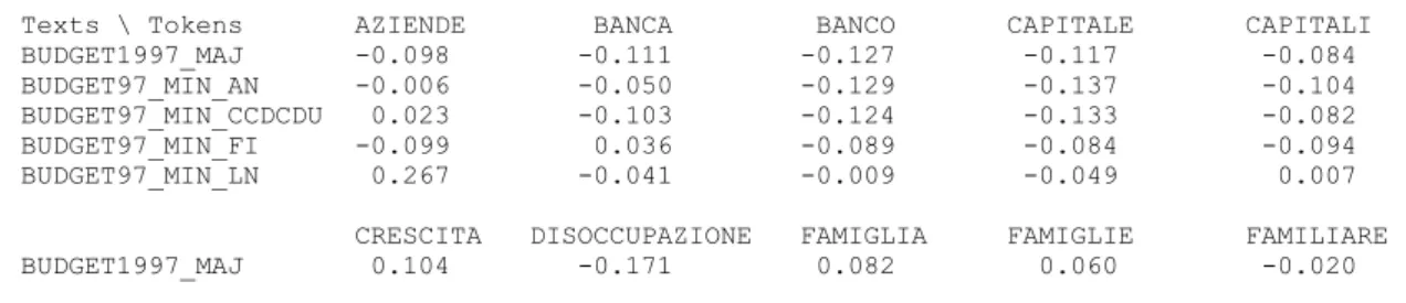
Table 2. SVD in three dimensions of documents by words scores matrix

Texts \ Tokens AZIENDE BANCA BANCO CAPITALE CAPITALI BUDGET1997_MAJ -0.098 -0.111 -0.127 -0.117 -0.084

BUDGET97_MIN_AN -0.006 -0.050 -0.129 -0.137 -0.104 BUDGET97_MIN_CCDCDU 0.023 -0.103 -0.124 -0.133 -0.082 BUDGET97_MIN_FI -0.099 0.036 -0.089 -0.084 -0.094 BUDGET97_MIN_LN 0.267 -0.041 -0.009 -0.049 0.007

CRESCITA DISOCCUPAZIONE FAMIGLIA FAMIGLIE FAMILIARE BUDGET1997_MAJ 0.104 -0.171 0.082 0.060 -0.020

8 Carroll, Green and Schaffer(1986) proposed analysing the indicator matrix associated with

the ‘pseudo-contingency table’. This is commonly termed ‘multiple’ or ‘canonical correspondence analysis’ (Greenacre, 1989:359; de Leeuw, Mair, 2009), but Weller and Romney (1990:66-68), quoting Nishisato and Sheu (1980), have shown it to be essentially the same thing as applying ‘simple

correspondence analysis’ to the original contingency table. The canonical scores (principal component values) are the same, although possibly reflected and rotated; the singular values appear to be different but are related by a simple formula R c 2 = (2RI2 - 1) 2 where R c is the singular value from

the contingency table analysis and RI is the first non-trivial singular value from the indicator matrix

BUDGET97_MIN_AN 0.072 0.048 -0.024 -0.018 -0.094 BUDGET97_MIN_CCDCDU 0.086 0.083 0.029 -0.007 -0.058 BUDGET97_MIN_FI 0.035 -0.137 -0.060 0.006 -0.088 BUDGET97_MIN_LN -0.013 0.547 -0.062 -0.128 -0.057

FAMILIARI FISCAL FISCALE FISCALI FISCALITÀ BUDGET1997_MAJ 0.017 -0.026 0.237 -0.159 -0.074

BUDGET97_MIN_AN -0.100 -0.125 0.461 -0.056 -0.112 BUDGET97_MIN_CCDCDU -0.047 -0.089 0.459 -0.135 -0.091 BUDGET97_MIN_FI -0.101 -0.096 0.184 0.059 -0.089 BUDGET97_MIN_LN -0.097 -0.112 0.512 -0.031 -0.033

IMPRENDITORI IMPRENDITORIALITÀ IMPRESA IMPRESE LAVORI BUDGET1997_MAJ -0.036 -0.063 0.039 -0.055 -0.100

BUDGET97_MIN_AN -0.117 -0.119 -0.050 0.126 -0.058 BUDGET97_MIN_CCDCDU -0.080 -0.099 -0.013 0.104 -0.112 BUDGET97_MIN_FI -0.101 -0.083 -0.055 0.033 0.041 BUDGET97_MIN_LN -0.072 -0.073 -0.077 0.316 -0.081

LAVORO MERCATI MERCATO OCCUPAZIONE OPPORTUNITÀ BUDGET1997_MAJ 0.523 0.024 -0.040 0.341 -0.031

BUDGET97_MIN_AN 0.376 -0.017 0.033 0.259 -0.086 BUDGET97_MIN_CCDCDU 0.514 0.041 0.033 0.305 -0.049 BUDGET97_MIN_FI 0.055 -0.095 -0.014 0.117 -0.093 BUDGET97_MIN_LN 0.164 0.083 0.151 0.009 -0.017

PENSIONI POVERI PRODURRE PRODURRÀ PRODUTTIVA BUDGET1997_MAJ -0.036 -0.133 -0.041 -0.127 -0.036

BUDGET97_MIN_AN -0.117 -0.100 -0.069 -0.129 -0.117 BUDGET97_MIN_CCDCDU -0.080 -0.138 -0.065 -0.124 -0.080 BUDGET97_MIN_FI -0.101 -0.010 -0.038 -0.089 -0.101 BUDGET97_MIN_LN -0.072 -0.060 -0.054 -0.009 -0.072

PRODUTTIVE PRODUTTIVI PRODUTTIVO PRODUZIONE PRODUZIONI BUDGET1997_MAJ -0.047 -0.020 -0.127 -0.041 -0.031

BUDGET97_MIN_AN -0.049 -0.038 -0.129 -0.069 -0.086 BUDGET97_MIN_CCDCDU -0.055 -0.060 -0.124 -0.065 -0.049 BUDGET97_MIN_FI -0.020 0.023 -0.089 -0.038 -0.093 BUDGET97_MIN_LN -0.028 -0.104 -0.009 -0.054 -0.017

PUBBLICA PUBBLICI PUBBLICO RICERCA SOCIALE BUDGET1997_MAJ 0.253 -0.052 0.130 -0.031 0.398

BUDGET97_MIN_AN 0.045 0.134 -0.000 -0.040 0.149 BUDGET97_MIN_CCDCDU 0.172 -0.007 0.078 -0.027 0.276 BUDGET97_MIN_FI -0.101 0.248 -0.078 -0.043 -0.017 BUDGET97_MIN_LN -0.042 -0.016 -0.035 0.012 -0.108

SOCIALI SVILUPPO TASSA TASSAZIONE TASSE BUDGET1997_MAJ 0.056 0.041 -0.126 -0.138 0.014

BUDGET97_MIN_AN 0.016 0.285 0.326 -0.071 0.223 BUDGET97_MIN_CCDCDU 0.091 0.116 -0.040 -0.152 0.080 BUDGET97_MIN_FI -0.106 0.366 0.644 0.070 0.297 BUDGET97_MIN_LN 0.139 0.042 -0.104 -0.111 0.038

TASSI TASSO UTILE UTILIZZARE UTILIZZATE BUDGET1997_MAJ 0.145 0.066 -0.036 -0.062 -0.133

BUDGET97_MIN_AN 0.060 0.068 -0.117 -0.045 -0.100 BUDGET97_MIN_CCDCDU 0.069 0.022 -0.080 -0.072 -0.138 BUDGET97_MIN_FI 0.062 0.125 -0.101 0.012 -0.010 BUDGET97_MIN_LN -0.136 -0.120 -0.072 -0.050 -0.060

Structures of co-occurrences in traditional content analysis

Co-occurrence of terms in texts is, of course, to be defined only in relation to some specified unit of context with which individual and joint occurrences, if necessary also joint

non-occurrences, are to be enumerated. It usually makes a difference, for example, if word pairs are counted within groups of three or more sentences, or single sentences (Smith,

level. It is essential to test the stability of the results obtained under variation of this important parameter, rather than adopt a single value in all circumstances. Once a reasonably stable matrix of co-occurrences of a set of items has been calculated, it is a simple matter to apply an appropriate coefficient of similarity to take joint non-occurrences into account and

compare the results obtained by excluding them from consideration.9

Equally fundamental is control over the means adopted to determine words in a text which are to be ignored, and/or explicitly included, in looking for structures of co-occurrence. Whatever strategy is adopted, the object is to determine a reduced list of individual words, or categories, to use as the basis for a series of classificatory methods (usually including clustering, multidimensional scaling/network analysis, and correspondence analysis) in the hope of uncovering structural relationships between them. If, however, a default stoplist applying normal considerations of triviality is accepted to speed up the process, there is always a chance that certain words or phrases, even, for example “yes, we can”, will automatically be excluded from the process of enumeration. On the other hand, “ich bin ein Berliner” stands a good chance of being correctly identified, in the speech of another prominent US politician visiting Germany in June 1963 as these words are unlikely to be excluded. It is particularly important to notice that the inclusion or exclusion of individual items can have significant effects on stability of the results of subsequent analytical

procedures (Smith, Humphreys :265ff.). We are therefore concerned to read the nonchalant claim “... that only function words are discarded from the analysis in Alceste.” (BWB, :597). Depending on the material to be analysed, this can make the difference between correct retrieval of significant content and actively misleading results.

‘Topics’ or clusters?

As an initial approach, it has often been found attractive (BWB: 592ff) to review the information about co-occurrences of words as a series of increasing numbers of clusters. HAMLET II offers an efficient non-hierarchical clustering algorithm (Brusco, 2003) which performs a similar function. Brusco’s method explicitly seeks to optimise the presentation order, and subsequently partitions the co-occurrence matrix into increasing numbers of clusters, each containing at least one item. Clusters are mutually exclusive, and exhaustive, in that all items are assigned to exactly one cluster. Unfortunately, given the number of ties that can occur in minimum diameter partitioning, it is likely that there are many alternative optima in large matrices. It is therefore advisable to compare the results obtained by this method with those from hierarchical clustering as well as with those of multidimensional scaling of the same matrix.

An example

In the work already cited (De Giorgi, 2008) the following set of categories, each defined by a number of words related to the theme indicated, was developed on the basis of the word

9

cij = (fij + t - ( fi + fj –fij)) / t (1)

where fij are the joint frequencies and fi, fj the individual frequencies of words i and j of words i and j in a given vocabulary list, expressed in units of context in each case, and t = ( fi + fj –fij), with those of the Jaccard coefficient (2)

sij = (fij) / (fi+ fj- fij), (2)

distributions of the party contributions to the opening debate on the 1997 Italian Budget to produce co-occurrence matrices for each party. The main interest of the investigation was a comparative study of the behaviour of parties in government and opposition in different EU countries and across a number of issue areas10_.

Main entry Associated words

Capitale Banc*, capital*, mercat*, produttiv*, profit

Lavoro Disoccupa*, lavor*, occupa*

Private Aziend*, imprenditor*, impres*, industria*, privat*

Pubblico Prestazion*, public*, servizi*

Sociale Ammortizzator*, famigli*, familiar*, pension*, pover*, social*, solida*,welfare Sviluppo Crescita, produ*, ricerc*, svilupp*, util*

Tasse Detass*, fisc*, tass*

Uguaglianza Eguaglianza, egual*, opportunit*, ugual*

Table 3 shows the frequencies for the above eight categories for the recorded contributions of the governing majority and the four minority opposition groups in the opening debate on the Italian budget of 1997

Table 3: Profiles of category frequencies for 1997 Italian budget debate speeches by party group11

Capitale Lavoro Privato Pubblico Sociale Sviluppo Tasse Uguagli-anza

Maj 3 9 5 9 12 9 11 1

AN 3 11 4 1 5 11 13 0

CCDCDU 2 11 5 5 8 9 9 2

FI 2 4 3 8 4 10 24 1

LN 19 22 22 9 12 23 20 2

The matrices of co-occurrences, however, vary between the various party contributions, so that comparing them provides access to differences in the contexts in which these terms occur. The most comprehensive comparison is possible in two stages, which can, of course be combined computationally, but are here separated to show the principles involved.

The first stage applies standard non-metric multidimensional scaling, treating the

standardised co-occurrence values as similarities, with the convenience that the results can be visualised in two or three dimensions, preserving the rank order of the original similarities. Figure 2 shows the result of this procedure applied to the contribution on behalf of the

majority coalition.

Figure 2 : Multidimensional scaling for the governing majority

The second stage, Procrustean Individual Differences Scaling (PINDIS) (Borg, Groenen, 2005 :477-492) allows direct and detailed comparison of structural relationships between the categories, as reflected in the set of configurations produced by applying MDS to each of the texts.

Figure 3 : PINDIS centroid configuration - centred and normed

If the GPA model aloneprovides a good enough fit between the centroid and the individual configurations to be compared, any further modelling, for example involving differential dimensional weighting, clearly becomes superfluous. In this sense, PINDIS can also be regarded as a kind of confirmatory data analysis (Commandeur 1991:164).

The PINDIS subject space (Figure 4) comparing the standardised co-occurrence matrices of the same categories for the budget debate speeches distinguishes them in a similar way to a correspondence analysis by rows of Table 3. Vectors are indicated in the plot as this is a vector space and cannot be interpreted in terms of Euclidean distances between the points representing the various parties. To analyse these differences in Euclidean terms, it is possible to transform them to arc-distances on a sphere of unit radius using the SUBJSTAT procedure, due to Forrest Young (1981). This can also apply an approximate test of the significance of hypothetical clusters which may be proposed among the configurations considered by PINDIS.

The mean subject communality of the normalized dimension weights represented here in relation to the centroid is 0.69, which confirms that the individual party contributions are indeed relatively heterogeneous. The fits of the subsequent transformations applied by PINDIS improve dramatically as the constraints of orthogonal normality are relaxed, to an overall average of 0.87 for the so-called 'perspective' models. These allow the vectors representing the individual categories for each subject to be separately re-positioned. Since weighting the vectors has the effect of pushing the stimulus points away towards the

periphery or pulling them closer towards the origin of the 3-dimensional reference space, these models offer the unique possibility of identifying highly specific differences in the centrality of certain terms in a series of texts.

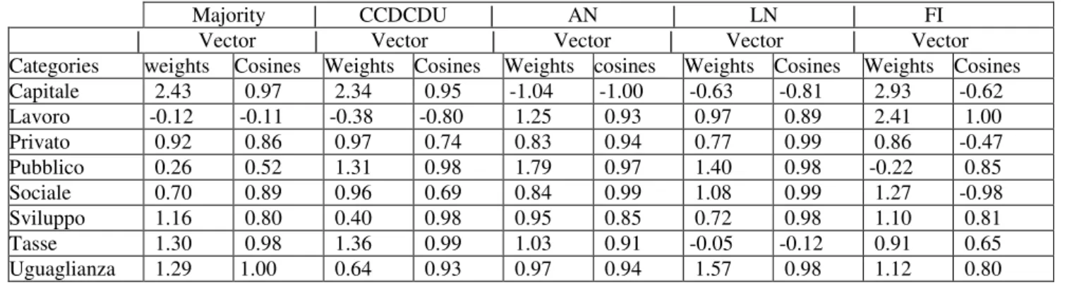
Table 4: PINDIS 'perspective' model - Vector weights and direction cosines*

Majority | CCDCDU | AN | LN | FI | Vector | Vector | Vector | Vector | Vector Categories weights Cosines Weights Cosines Weights cosines Weights Cosines Weights Cosines Capitale 2.43 0.97 2.34 0.95 -1.04 -1.00 -0.63 -0.81 2.93 -0.62 Lavoro -0.12 -0.11 -0.38 -0.80 1.25 0.93 0.97 0.89 2.41 1.00 Privato 0.92 0.86 0.97 0.74 0.83 0.94 0.77 0.99 0.86 -0.47 Pubblico 0.26 0.52 1.31 0.98 1.79 0.97 1.40 0.98 -0.22 0.85 Sociale 0.70 0.89 0.96 0.69 0.84 0.99 1.08 0.99 1.27 -0.98 Sviluppo 1.16 0.80 0.40 0.98 0.95 0.85 0.72 0.98 1.10 0.81 Tasse 1.30 0.98 1.36 0.99 1.03 0.91 -0.05 -0.12 0.91 0.65 Uguaglianza 1.29 1.00 0.64 0.93 0.97 0.94 1.57 0.98 1.12 0.80

*Note: Weights are the lengths of the fitted vectors; direction cosines range from 1.0 for the identical direction, to -1.0, meaning the fitted vector is in exactly the opposite direction from the centroid for all texts.

Although Table 4 may look complicated, the most substantial differences between the various party positions are immediately apparent from very small or negative vector weights and direction cosines, indicating that the corresponding stimuli have substantially different associations or emphases for the groups concerned, when compared to the mean configuration for all speeches. In addition, some similar patterns of deviation from the centroid are apparent, for example, for the majority and the CCDCDU, for the categories 'capitale' and 'lavoro', which distinguish these two groups from the rest. LN and AN are also similar, but LN has a divergent treatment of ‘tasse’. FI, on the other hand, has a pattern of its own, according to the results of this PINDIS model.

In conclusion

In comparing structures of relationships between words or categories between texts, PINDIS has the almost unique12 _{advantage of identifying the particular words or categories concerned} in any structural differences to be observed between the parties. Using PINDIS, as described here, to compare the configurations obtained by non-metric scaling of matrices of co-occurrences yields more detailed, reliable and potentially testable information than the common application of the metric procedure correspondence analysis in comparing profiles of word or category counts for the same series of texts.

In visualising the results of both approaches, restriction to a maximum of three dimensions can be misleading. Correspondence analysis in particular raises the difficulty that the conventional plotting of row and column variables of the original data matrix superimposed in the same space does not imply that relationships between them are open to interpretation according to inter-set distances. “The interpretation of correspondence analysis is by no means a trivial exercise. The technique is tremendously useful in the analysis of marketing data, but its limitations should be fully realized and clearly understood. Experience is needed to extract valid information from the displays and the underlying geometry should always be borne in mind.” (Greenacre 1989, 364).

We also should not confuse issues of convenience in representation and visualisation of relationships in the data with those of interpretation and analysis. The distinction between ‘automatic’ and ‘semi-automatic’ is unhelpful in developing an appropriate understanding of the issues arising in this kind of research. Although Alceste and similar software invites a kind of universal, unreflecting approach irrespective of the nature of the material to be studied, we remain unconvinced by the claim that prior theoretical considerations have no place in this kind of systematic political science research.

In conclusion it might be suggested that the two strategies should preferably be employed in a complementary manner. Following an interesting suggestion of Reinhold Rapp (1999), they may be seen in relation to Saussure’s distinction (1916) between paradigmatic and syntagmatic word associations. Paradigmatic associations involve words with high semantic similarity (Ruge 1992), which can be computed by determining the similarity of their lexical neighbourhoods. The relation between two words is paradigmatic if they can be substituted for each other in a sentence without affecting its grammatical structure or acceptability in a language, typical cases being synonyms or antonyms. Rapp shows that both are reflected in the statistical distribution of words in large corpora. In this view, it can be suggested that his second-order associations identified using log-likelihood ratios to determine the primary associative response for each word in relation those occurring in its vicinity, and the topic allocations of LDA are to be regarded as syntagmatic. The first-order associations expressed by co-occurrences of specified word pairs used to compute similarities contain a combination of paradigmatic and syntagmatic associations. Extracting the former from the latter should produce the purely syntagmatic.

12 Another approach, using source material provided by Reuters news agency over the 66 days

between September 11 and November 15, 2001 (Johnson,Krempel 2004; Diesner, Carley 2004) uses Centering Resonance Analysis (CRA, Corman et al. 2002) which determines the structure of

relationships between the words making up noun-phrases (anything consisting of a noun plus zero or more nouns and adjectives) occurring within individual sentences of the text source and transforms them into a semantic network. The authors nevertheless found it necessary to make an essentially qualitative simplification of the networks analysed over time by recoding the individual words occurring into one of six categories, to be able to apply the molecular visualisation programme ’Mage’

Appendix: The transformations applied in PINDIS (Lingoes and Borg,1978)

Given a set of n configurations Xj (j = 1...n) of order (p x m) containing the co-ordinates of

the same p stimuli in m dimensions, if Rj is an orthonormal matrix of order (m x m), sj a central dilation and uj a translation vector of order (1 x m), defining Z as a group or centroid configuration of order (p x m), E j as a (p x m) matrix of residuals and l as a (p x 1) vector of ones, the GPA model can be formulated as

sj (Xj-1u´j)R = Z + Ej , for j = 1...n

If Qj, S,and Sj are unknown orthonormal matrices of order (m x m), gj and hj unknown

translation vectors of order (m x 1), and Wj is an unknown diagonal matrix of order (m x m),

PINDIS offers the dimensional weighting model

( Xj– 1g΄j ) Q j = (Z–1h΄j ) SWj+ Ej , for j = 1...n,

followed by dimensional weighting with individual rotation of the centroid Z

( Xj– 1g΄j) Q j = (Z–1h΄j ) SjWj+ Ej , for j = 1...n.

Two further models consider the variables of the individual configurations as vectors from the origin of the centroid, which is assumed to be fixed. With gj, h and hj unknown translation

vectors of order (m x 1), Tj an unknown orthonormal matrix of order (m x m), and Vj an

unknown diagonal matrix of order (p x p), the fourth (variable vector lengths) can be written as

( Xj– 1g΄j ) T j = Vj (Z–1h΄ ) SWj+ Ej , for j = 1... n,

and the fifth (variable vector lengths and direction cosines) as

( Xj– 1g΄j ) T j = Vj (Z–1h΄j ) SWj+ Ej , for j = 1... n.

The centroid configuration Z is assumed to be fixed. The diagonal matrices Vj have the effect

of differentially weighting the vectors represented by the stimulus points in (Z–1h΄) or (Z– 1h΄j ). Z is translated only once for the vector weighting model, but differently for each

configuration in the fifth model listed..

References

Bara, J., Weale, A., Bicquelet,A. (2007) Swiss Political Science Review 13(4): 577–605. Benzécri, J.P. (1973) Analyse des données, Paris, Dunod.

Benoit, K., and M. Laver.(2003). Estimating Irish party positions using computer wordscoring: The 2002 elections. Irish Political Studies 17:97–107.

Blei, D.M., Ng, A.Y., Jordan, M.I. (2003) Latent Dirichlet Allocation, Journal of Machine Learning Research, 3, pp.993-1022.

Bourdieu, P. (1979) La distinction – critique sociale du jugement, Paris, Éditions de Minuit, Le Sens commun. Borg, I, Groenen, P. (2005) Modern Multidimensional Scaling: Theory and applications. Heidelberg: Springer, 3rd edition.

Brier, A.P., Hopp, B. (2011) Quantitative Analysis of Textual Data with HAMLET II 3.0 for Windows, Software Manual, [http://www.apb.newmdsx.com/hamlet23.pdf]

Brusco, M.J.(2003) An enhanced branch-and-bound algorithm for a partitioning problem. British Journal of Mathematical and Statistical Psychology, 56, pp. 83–92.

Carroll, J.D., Green, P.E., Schaffer, C.M. (1987). Comparing Interpoint Distances in Correspondence Analysis: A Clarification, Journal of Marketing Research, 24:445-50.

Carroll, J.D., Green, P.E., Schaffer, C.M. (1989): Reply to Greenacre’s Commentary on the Carroll -Green-Schaffer Scaling of Two-Way Correspondence Analysis Solutions, Journal of Marketing Research, 26:358-365. Chang, J.J. and Carroll,J.D. (1969) How to use MDPREF, a computer program for multidimensional analysis of preference data,. Computer Manual. Murray Hill, N.J., Bell Laboratories.

Commandeur, J.J.F. (1991) : Matching Configurations. Leiden University: DSWO Press, Leiden

Corman, S.R., Kuhn, T, McPhee, R.D., Dooley, K.J., (2002) Studying complex discursive systems. Centering resonance analysis of communication, Human Communication Research 28(2)

De Giorgi, E. (2008) Parliamentary opposition in Western European democracies today: systemic or issue-oriented? A comparative analysis of four parliamentary systems, PhD dissertation in Comparative and European Politics, University of Siena.

De Giorgi, E. (2011) L’opposition parlementaire en Italie et au Royaume Uni: systémique ou axée sur les enjeux?, in Revue Internationale de Politique Comparée, 18 (2): 93-113.

De Giorgi, E. and Marangoni F. (2015) Government laws and the opposition parties’ behaviour in parliament, Acta

Politica, 50 (1): 64-81.

Diesner, J., Carley, K.M. (2004) Using Network Analysis to Detect the Organizational Structure of Covert Texts, Proc. of the North American Ass. for Computational Social and Organizational Science (NAACSOS); 2004 Conference Pittsburgh, P.A.

Eckart, C. and Young, G.(1936) The approximation of one matrix by another of lower rank, Psychometrika, 1 : 211-218.

Everitt, B.S., Rabe-Hesketh, S. (1996) The Analysis of Proximity Data, London, Arnold.

Feinerer I, Hornik K, Meyer D (2008). Text Mining Infrastructure in R. Journal of Statistical Software, 25(5) [http://www.jstatsoft.org/v25/i05]

Fisher, R.A. (1940) The precision of discriminant functions, Annals of Eugenics, 10:422-429.

Gilks, W. R., Richardson, S., & Spiegelhalter, D. J. (1996). Markov chain Monte Carlo in practice. London: Chapman & Hall.

Gower, J.C. (1975) Generalized procrustes analysis, Psychometrika, 40 : 33-51.

Gower J.C., Hand, D.J. (1996). Biplots. Monographs on Statistics and Applied Probability. Chapman & Hall, London

Greenacre, M.J. (1989): The Carroll-Green-Schaffer Scaling in Correspondence Analysis: A Theoretical and Empirical Appraisal, Journal of Marketing Research, 26:358-365.

Griffiths, T. L., & Steyvers, M. (2004). Finding scientific topics. Proceedings of the National Academy of Science, 101, 5228-5235.

La Grange, A. (2010) Vignette: BiplotGUI [www.cran.r-project.org/web/packages/BiplotGUI/BiplotGUI.pdf] Grün,B., Hornik,K. (2010): topicmodels: An R Package for Fitting Topic Models, Comprehensive R Project Network [http://cran.r-project.org/web/packages/topicmodels/vignettes/topicmodels.pdf]

Hotelling, H.(1935) The most predictable criterion, Journal of Educational Psychology, 26:139-142. Hotelling, H.(1936) Relations between two sets of variates, Biometrika, 28:321-377.

Italian Chamber of Deputies (1997) L. 663/96, Legge finanziaria 1997, (C. 2371) Seduta giovedì 31 ottobre 1996 (inizio esame in aula)

Johnson, J.C., Krempel , L. (2004) Network Visualization: The "Bush Team" in Reuters News Ticker 9/11-11/15/01, Journal of Social Structure, 5 (1).

Landmann, J., Züll, C. (2004) Computer Assisted Content Analysis without a dictionary? in: van Dijku, C, Blasius, J., Kleijer, H. (eds.) Recent Developments and Applications In Social Research Methodology. Proceedings of the Sixth International Conference on Logic and Methodology, Amsterdam: SISWO. Langeheine, R. (1980) Approximate Norms and Significance Tests for the LINGOES-BORG Procrustean

Individual Differences Scaling (PINDIS), Institut für die Pädagogik der Naturwissenschaften. University of Kiel Langeheine, R. (1982) Statistical evaluation of measures of fit in the Lingoes-Borg Procrustean individual differences scaling, Psychometrika, 47:423-442.

Laver,M., Garry,J.(2000) Estimating policy positions from political texts, American Journal of Political Science 44(3) pp.619-634.

Laver,M., Benoit,K. Garry,J.(2003) Extracting Policy Positions from Political Texts Using Words as Data. American Political Science Review 97(2): 311–32.

Lewis, Maas (2007) QDA Miner 2.0: Mixed-Model Qualitative Data Analysis Software, Field Methods, 19: 87-108

de Leeuw, J, Mair, P. (2009). Simple and Canonical Correspondence Analysis Using the R Package anacor, Journal of Statistical Software 31(5):1-18.

Lingoes, J.C., Borg, I (1978) A direct approach to individual differences scaling using increasingly complex transformations, Psychometrika, 43

Lowe, W., Benoit, K., Mikhaylov, S.,Laver,M. (2011) Scaling policy positions from coded units of political texts Legislative Studies Quarterly 36(1).

Monroe, B.L., Schrodt, P.A.(2008) Introduction to the special issue: The Statistical Analysis of Political Texts, Political Analysis 16 (4):351-355

Microsystems Limited (2001): TextAnalyst [ http://www.analyst.ru].

Nishisato,S, Sheu ,W. (1980) Piecewise method of reciprocal averages for dual scaling of multiple-choice data, Psychometrika, 45 :467-478.

Osgood, C., Suci, G.J., Tannenbaum, P.H. (1957) The Measurement of Meaning, Urbana, Ill., University of Illinois Press.

Proksch, S.-O., Slapin, J.B. (2009) How to Avoid Pitfalls in Statistical Analysis of Political Texts: The Case of Germany, German Politics, 18: 3, 323-344

Provalis Research, Montreal, Canada [http://www.provalisresearch.com]

Rapp, R. (2002) The Computation of Word Associations: Comparing Syntagmatic and Paradigmatic Approaches, COLING – 19th _{International Conference on Computational Linguistics, Taipei.}

Reinert,M. (2005) Alceste: Manuel d’ulitisation, Toulouse, Image [http://www.image.cict.fr/english/index.htm] Ruge, G. (1992). Experiments on Linguistically Based Term Associations. Information Processing & Management 28(3), 317–332.

de Saussure, F. (1916/1996). Cours de linguistique générale. Paris: Payot.

Schonhardt-Bailey, C. (2005). Measuring Ideas More Effectively: An Analysis of Bush and Kerry’s National

Security Speeches. Political Science and Politics 38(4).

Slapin, J. B., S.-O. Proksch. (2008) A scaling model for estimating time-series party positions from texts. American Journal of Political Science 52:705–22.

Sokal, R.R., Sneath, P.H. (1963) Principles of Numerical Taxonomy, New York , Freeman.

Steyvers,M., Griffiths,T. (2007) Probabilistic Topic Models, in Landauer,T., McNamara,D., Dennis,S., Kintsch,W. (eds), Latent Semantic Analysis: A Road to Meaning, Laurence Erlbaum, Hillsdale, N.J.

Smith, A.E., Humphreys, M.S. (2006) Evaluation of unsupervised semantic mapping of natural language with Leximancer concept mapping, Behavior Research Methods, 38(2):262-279.

Verzichelli, L., Cotta, M. (2000) Italy: From "Constrained" Coalitions to Alternating Governments?, in: Müller, W.C., Strøm, K. (eds.) Coalition Governments in Western Europe, Oxford, Oxford University Press. Weller, S.C., Romney, A.K. (1990) Metric Scaling, London: Sage Publications, Quantitative Applications in the Social Sciences; no. 75.

Young, F.W. (1981) in Schiffman, S.S., Reynolds, M.L, Young, F.W. Introduction to Multidimensional Scaling. Theory, Methods and Applications. New York: Academic Press : 314-318.