A modeling approach to determine the impacts of land use and climate change scenarios on the water flux of the upper Mara River

(1)

HESSD

7, 5851–5893, 2010

Impacts of land use and climate change scenarios on water

flux

L. M. Mango et al.

Title Page

Abstract Introduction

Conclusions References

Tables Figures

◭ ◮

Back Close

Full Screen / Esc

Printer-friendly Version Interactive Discussion

Discussion

P

a

per

|

Dis

cussion

P

a

per

|

Discussion

P

a

per

|

Discussio

n

P

a

per

|

Hydrol. Earth Syst. Sci. Discuss., 7, 5851–5893, 2010 www.hydrol-earth-syst-sci-discuss.net/7/5851/2010/ doi:10.5194/hessd-7-5851-2010

Hydrology and Earth System Sciences Discussions

This discussion paper is/has been under review for the journal Hydrology and Earth System Sciences (HESS). Please refer to the corresponding final paper in HESS if available.

A modeling approach to determine the

impacts of land use and climate change

scenarios on the water flux of the upper

Mara River

L. M. Mango1, A. M. Melesse2, M. E. McClain3, D. Gann1, and S. G. Setegn2

1

Geographic Information Systems-Remote Sensing Center, Florida International University, Miami, FL 33199, USA

2

Department of Earth and Environment, Florida International University, Miami, FL 33199, USA

3

Department of Water Engineering, UNESCO-IHE Institute for Water Education, Delft, The Netherlands

Received: 8 June 2010 – Accepted: 30 July 2010 – Published: 17 August 2010

Correspondence to: L. M. Mango (lm mango@yahoo.com)

(2)

HESSD

7, 5851–5893, 2010

flux

L. M. Mango et al.

Title Page

Tables Figures

◭ ◮

Back Close

Full Screen / Esc

Discussion

P

a

per

|

Dis

cussion

P

a

per

|

Discussion

P

a

per

|

Discussio

n

P

a

per

Abstract

With the flow of the Mara River becoming increasingly erratic especially in the upper reaches, attention has been directed to land use change as the major cause of this problem. The semi-distributed hydrological model Soil and Water Assessment Tool (SWAT) and Landsat imagery were utilized in the upper Mara River Basin in order to

5

1) map existing field scale land use practices in order to determine their impact 2) determine the impacts of land use change on water flux; and 3) determine the impacts of rainfall (0%,±10% and±20%) and air temperature variations (0% and+5%) based on the Intergovernmental Panel on Climate Change projections on the water flux of the upper Mara River.

10

This study found that the di_fferent scenarios impacted on the water balance compo-nents differently. Land use changes resulted in a slightly more erratic discharge while rainfall and air temperature changes had a more predictable impact on the discharge and water balance components. These findings demonstrate that the model results show the flow was more sensitive to the rainfall changes than land use changes. It

15

was also shown that land use changes can reduce dry season flow which is the most important problem in the basin. The model shows also deforestation in the Mau Forest increased the peak flows which can also lead to high sediment loading in the Mara River. The effect of the land use and climate change scenarios on the sediment and water quality of the river needs a thorough understanding of the sediment transport

20

processes in addition to observed sediment and water quality data for validation of modeling results.

1 Introduction

Water is an extremely important resource in Kenya and is the lifeline of its ecosystems. It is used for agriculture, industry, power generation, livestock production, and many

25

(3)

HESSD

7, 5851–5893, 2010

flux

L. M. Mango et al.

Title Page

Tables Figures

◭ ◮

Back Close

Full Screen / Esc

Discussion

P

a

per

|

Dis

cussion

P

a

per

|

Discussion

P

a

per

|

Discussio

n

P

a

per

|

(SoK, 2003) and most of this is supplied by the country’s rivers most of which are concentrated in the highlands. In terms of water supply, Kenya receives seasonally and annually variable marginal rainfall with an annual average rainfall of 630 mm which is relatively low for an equatorial country (FAO, 2005). It is also categorized as a water scarce country based on the average per capita water availability (WRI, 2007) and this

5

is a major challenge to the country in several ways. The scarcity of this crucial resource therefore necessitates its quantification, and maintenance of adequate flows.

The 395 km long Mara River is transboundary and drains an area of about 13, 750 km2 across the Kenya-Tanzania border, the Mara Basin (Mati et al., 2005). Widespread human activities such as cultivation and deforestation of the Mau

catch-10

ment in the highlands have led to erratic flow in the Mara River in both the dry and wet seasons and this is a problem considering the high demand for water by the large populations of Mara Basin inhabitants. Downstream of the Mara River are human settlements, agricultural areas, protected areas that support immense wildlife popu-lations and wetlands that are dependent on the availability of this water in adequate

15

quality and quantity. Activities such as deforestation, irrigation and the construction of weirs on tributaries of the Mara such as the Amala River may reduce the flow of the Mara river to a halt during severe droughts and this reduction in quantity and quality greatly impacts wildlife-water interactions and consequently, the ecology of ecosys-tems such as the Mara river basin (Gereta and Wolanski, 1998, 2002). Serneels et

20

al. (2001) in a study of land cover changes in the Mara ecosystem, noted that climatic, anthropogenic and other factors shape the vegetation, ecology and biodiversity of an ecosystem. According to Mutie et al. (2006), modification of natural land cover and soil conditions have brought about changes in the river flow regime such as high peak flows, reduced baseflows, enlarged river channel and silt deposition downstream.

Reli-25

(4)

HESSD

7, 5851–5893, 2010

flux

L. M. Mango et al.

Title Page

Tables Figures

◭ ◮

Back Close

Full Screen / Esc

Discussion

P

a

per

|

Dis

cussion

P

a

per

|

Discussion

P

a

per

|

Discussio

n

P

a

per

and maximum river flows sufficient for all the stakeholder needs.

The specific objectives of this study were to: map existing land use practices using remote sensing and field observations, determine the impacts of land use change, rain-fall and air temperature variation on the water flux of the upper Mara River in Kenya. The findings of this study provided scenarios on the impacts of land use and climate

5

change in the upper Mara River Basin therefore adding to the existing literature and knowledge base with a view of promoting better land use management practices in Kenya and application of the SWAT model in similar densely populated, highly agricul-tural watersheds all over the world.

2 Methods

10

For the SWAT model application in the upper Mara Basin, detailed dataset inputs had to be prepared. These datasets included detailed land use/land cover map, soil classi-fication map, and climate data on a daily time-step. The land use map is an important input for the model and involved analysis of remote sensor data in order to generate a detailed accurate map for use in the SWAT model.

15

2.1 Study area

The transboundary Mara River Basin is shared between Kenya and Tanzania and is located in East Africa between longitudes 33.88372◦ _{and 35.907682}◦ _{West, latitudes}

−0.331573◦and−1.975056◦South. It covers about 13 750 km2(Mati et al., 2005) and is characterized by different types of land cover and land uses as a result of different

20

human activities carried out by the stakeholders in various parts of the basin. The land uses include; urban settlements and villages, subsistence and large scale agriculture, forestry, livestock, fisheries, tourism, conservation areas, mining and other industries. The Mara River flows from its catchment in the high altitude Mau Forest in Kenya across different landscapes and finally drains into Lake Victoria at Musoma Bay in Tanzania.

(5)

HESSD

7, 5851–5893, 2010

flux

L. M. Mango et al.

Title Page

Tables Figures

◭ ◮

Back Close

Full Screen / Esc

Discussion

P

a

per

|

Dis

cussion

P

a

per

|

Discussion

P

a

per

|

Discussio

n

P

a

per

|

2.2 SWAT model description

The Soil and Water Assessment Tool (SWAT) is a hydrological model that can be ap-plied at the river basin, or watershed scale. It was developed for the purpose of sim-ulation of impact of land management practices on water, sediment and agrochemical yields in large watersheds with varying soils, land use and agricultural conditions over

5

extended time periods (Neitsch et al., 2005). Arnold et al. (1998) defines SWAT as a semi-distributed, time continuous simulator operating on a daily time step. It is de-veloped for assessment of the impact of management and climate on water supplies, sediment, and agricultural chemical yields in sub-basins and larger basins. The pro-gram is provided with an interface in Arc View GIS (Di Luzio et al., 2002) for the

def-10

inition of watershed hydrologic features and storage, as well as the organization and manipulation of the related spatial and tabular data.

2.3 Land use data classification

The SWAT model requires a spatially explicit land use map as an input in order to sim-ulate the hydrology of a watershed. Land use data was obtained by the classification of

15

remote sensor data specifically, satellite imagery from the Landsat 4/5 Thematic Map-per (TM) sensor built for earth observation purposes. Both its spatial resolution of 30 m pixel and 7 band radiometric resolution make it suitable for land cover classification (Van der Meer et al., 2002). Two images of Path 169, Row 61 and Path 169, Row 60 from the 5 September 2008 were selected for the classification.

20

The imagery was prepared by subsetting, mosaicking and atmospheric correction that was required to remove haze and cloud from the image and also to convert the image from radiance to scaled surface reflectance values required for use in the land cover/land use classification. Atmospheric correction was carried out by ATCOR 2 of the ATmospheric CORrection (ATCOR) module in ERDAS IMAGINE that consists of

25

(6)

HESSD

7, 5851–5893, 2010

flux

L. M. Mango et al.

Title Page

Tables Figures

◭ ◮

Back Close

Full Screen / Esc

Discussion

P

a

per

|

Dis

cussion

P

a

per

|

Discussion

P

a

per

|

Discussio

n

P

a

per

Land cover classification was carried out by means of a machine learning algorithm that makes use of recursive partitioning. The pixel spectral values and spatial locations of different land cover classes were extracted from the atmospherically corrected image and saved in a table. The reflectance data was then loaded into the statistical pack-age R (RDCT, 2009) that performed the classification of the data by means of recursive

5

partitioning script. A cross-validation which involves hiding the classes obtained one at a time and using the other resultant classes to predict their values statistically (Liu and Liu, 2008) was performed in 5 and 10 iterations, respectively, to increase the ac-curacy of the classification. The resulting decision tree and production rules were used to build an expert classifier in ERDAS IMAGINE 9.3 (ERDAS, 2006) used to perform a

10

classification of the image.

The expert classifier was constructed using the Knowledge Engineer Tool which in-volved identification of the hypotheses which are the classes identified in the study area; Cloud, Bushland, Cropland, Grassland, Bare soil, Shadow, Water and Forest. The expert system rules (variables) and conditions were specified based on remote

15

sensing multispectral reflectance characteristics and derivatives including the Kauth Thomas Tasseled Cap transformation and texture bands. The recursive partitioning process carried out beforehand resulting in the decision tree and production rules sig-nificantly reduced the time and effort required to construct the expert classifier which was then used to classify the image.

20

A land use/land cover classification scheme was formulated that would accurately and adequately represent the land cover/land use within the Mara River basin (Table 1). This scheme however follows the basic principles of the USGS Land use/land cover classification system (LULCCS) for use with remote sensor data level classification (Anderson et al., 1976).

25

2.4 Hydrological modeling

(7)

HESSD

7, 5851–5893, 2010

flux

L. M. Mango et al.

Title Page

Tables Figures

◭ ◮

Back Close

Full Screen / Esc

Discussion

P

a

per

|

Dis

cussion

P

a

per

|

Discussion

P

a

per

|

Discussio

n

P

a

per

|

specific information about weather, soil properties, topography, vegetation and land management practices which it uses as inputs to simulate the physical processes as-sociated with water movement, nutrient transport, crop growth and sediment move-ment. This enables it to model ungaged watersheds and more importantly, quantify the impact of alternative input data such as changes in land use, land management

prac-5

tices and climate on water quality and quantity. Secondly, it uses readily available data, while more inputs can be used to simulate more specialized processes it is still able to operate on minimum data which is an advantage especially when working in areas with insufficient or unreliable data. Third, the SWAT model is computationally efficient, able to run simulations of very large basins or management practices without consuming

10

large amounts of time and expenses. Lastly, it is a continuous time or a long-term yield model able to simulate long term impacts of land use, land management practices and build up of pollutants (Neitsch et al., 2005). These qualities of the SWAT model enabled the quantification of long term impacts of land use changes, variations in rainfall and air temperature on the hydrology of the Mara Basin.

15

2.4.1 DEM

The digital elevation model (DEM) of 90 m by 90 m resolution for the study area ob-tained from the Shuttle Radar Topography Mission (SRTM) was used. The DEM gives the elevation of a particular point at a particular spatial resolution and was used in the delineation of the watershed and analysis of the land surface characteristics and

20

drainage patterns.

2.4.2 Soil data classification

Soil data was obtained from the Soil Terrain Database of East Africa (SOTER). GIS layers were obtained and used in the hydrological model as one of the main inputs to the SWAT model which requires soil property data such as the texture, chemical

com-25

(8)

HESSD

7, 5851–5893, 2010

flux

L. M. Mango et al.

Title Page

Tables Figures

◭ ◮

Back Close

Full Screen / Esc

Discussion

P

a

per

|

Dis

cussion

P

a

per

|

Discussion

P

a

per

|

Discussio

n

P

a

per

density and organic carbon content for the different layers of each soil type (Setegn, 2008). A user table specific for the Mara River basin soil layer was appended to the soil table in the SWAT database by using Arc toolbox in ArcGIS since the soil types found in the study area are not included in the US soils database

2.4.3 Land use

5

Land use data for the year 2008 was obtained by analysis of Landsat TM imagery in the process described previously in this chapter resulting in land cover maps of the study area. These land cover maps were then converted to shapefiles and aggregated to make them easier to input into the model for use in the hydrological modeling exercise. Land use and management is an important factor affecting different processes in the

10

watershed such as surface runoff, erosion and evapotranspiration. Reclassification of the land use map was done in order to present them in a form that is acceptable in the model and this is the USGS Land use/ Land cover classification scheme for Use with Remote Sensor data level classification (Anderson et al., 1976).

2.4.4 Climate data 15

Climate data used in the SWAT model consists of daily rainfall, temperature, wind speed, humidity and evapotranspiration data. The weather variables used were the daily precipitation values obtained from the Bomet Water Supply Office Station located at Bomet Town and Kiptunga Forest Station located in Elburgon District, minimum and maximum air temperature values for the period of 1996–2003 obtained from the

Keri-20

cho Hail Research and Narok Meteorological weather stations. These data were ob-tained from the Ministry of Water Resources of Kenya and the Lake Victoria South Water Resource Management Authority in Kenya.

Another source of rainfall data for the hydrological modeling was obtained from the Famine Early Warning System (FEWS) Rainfall Estimation (RFE) imagery. This is a

25

(9)

HESSD

7, 5851–5893, 2010

flux

L. M. Mango et al.

Title Page

Tables Figures

◭ ◮

Back Close

Full Screen / Esc

Discussion

P

a

per

|

Dis

cussion

P

a

per

|

Discussion

P

a

per

|

Discussio

n

P

a

per

|

of 10 km (Xie and Arkin, 1996). The rainfall is obtained by means of a python script de-veloped by Gann (2008) which runs in an ArcGIS environment and extracts RFE statis-tics from daily rasters for user defined regions such as watersheds or sub-watersheds. Output is formatted to be compatible with input file format of ArcSWAT, in this case daily time series data tables in the ArcSWAT 2005 model input format. This process resulted

5

in the creation of 30 artificial rain gages as the centroids of the 30 sub-watersheds mak-ing up the Amala and Nyangores watersheds. Both the Amala and Nyangores water-sheds were assigned 15 RFE Rain gauges each for use in the hydrological modeling process. The RFE data was able to provide continuous and complete data ranging from the years 2002 to 2008 which was used in the model simulations.

10

2.4.5 River discharge

Daily river discharge data was obtained for the rivers Amala and Nyangores from the gauging stations located at the outlets of the basins. The discharge values for the two tributaries of the Mara; the Amala and Nyangores Rivers were used for calibration and validation of the model. In the Nyangores watershed, the available discharge data ran

15

from the year 1996 to the year 2008. For the rain gauge data model, out of that the 8 years of complete time series datasets 4 years were used for calibration and the remaining 4 years were used for validation. For the RFE model, 4 years were used for calibration and 3 for validation. In the Amala watershed, observed discharge data spanned from the year 2000 to 2006 and for the rain gauge model, 2 years were used

20

(10)

HESSD

7, 5851–5893, 2010

flux

L. M. Mango et al.

Title Page

Tables Figures

◭ ◮

Back Close

Full Screen / Esc

Discussion

P

a

per

|

Dis

cussion

P

a

per

|

Discussion

P

a

per

|

Discussio

n

P

a

per

2.4.6 Model run

To set up a hydrological SWAT model, basic data are required: topography, soil, land use and climatic data (Schuol et al., 2006). The model setup involved five steps: (1) data preparation, (2) sub-basin discretization, (3) HRU definition, (4) parameter sensitivity analysis, (5) calibration and uncertainty analysis.

5

The DEM was projected to the required projection parameter which is UTM Zone 37 South. A mask was used to reduce the area for stream delineation and analysis of terrain drainage patterns of the land surface. The streams were delineated from the DEM which accurately captured their true location on the ground. The land use/land cover layer was reclassified into the SWAT/USGS land use code as per required by the

10

model and linked to a user table with the land use code.

Watershed and sub-watershed delineation was carried out using the DEM and has various steps including: DEM setup, stream definition, outlet and inlet definition, wa-tershed outlets selection and definition and calculation of sub basin parameters. The resulting sub-watersheds were then divided into units based on their unique

combina-15

tion of land use, soils and slope combinations and these units are known as HRUs (hydrologic response units). The model was run on a default simulation of 8 years from 1996 to 2003 for the Rain gauge data and from 2002 to 2003 a period of two years for the RFE data.

2.5 Scenario analysis 20

2.5.1 Land use scenarios

To explore the sensitivity of SWAT outputs to land use and the effect of land use/land cover changes on the discharge of the Amala and Nyangores Rivers, land use sce-narios were explored. Attention was paid to ensure these were realistic scesce-narios in accordance to the ongoing trends of land use change within the study area. The

per-25

(11)

HESSD

7, 5851–5893, 2010

flux

L. M. Mango et al.

Title Page

Tables Figures

◭ ◮

Back Close

Full Screen / Esc

Discussion

P

a

per

|

Dis

cussion

P

a

per

|

Discussion

P

a

per

|

Discussio

n

P

a

per

|

land use scenarios included;

1. Partial deforestation

This scenario involved manipulation of the forest cover reducing it partially by converting the deciduous forest type to small scale or close grown agricultural land.

5

2. Complete deforestation

This scenario involved replacing all the existing forest cover with grassland to simulate a complete absence of forest cover in the watershed.

3. Conversion of forest to agriculture

Replacement of forest land by agriculture is a common trend within the study area

10

and is seen to be one of the major causes of erratic river flows and increased sediment load in the Nyangores and Amala Rivers. This scenario was carried out by replacing all forest cover with agriculture particularly small scale agriculture.

2.5.2 Climate change scenarios

According to the Intergovernmental Panel on Climate Change (2007), climate change

15

can be defined as an identifiable change in the state of the climate by change in the mean and/or variability of its properties and that persists for an extended period, typi-cally decades or longer.

Trends from 1900 to 2005 have been observed in precipitation and have seen a decrease in precipitation in the Sahel region which has been accounted for in the

pre-20

cipitation reduction scenarios carried out in this study. In the case of projection of future changes of changes in climate for the 21st century and beyond, consideration was given to the scenarios described in the IPCC Special Report on Emission Sce-narios and the scenario chosen for the region was A1Fl (rapid economic growth and fossil intensive). This was based on the fact that Kenya is a developing country with a

25

(12)

HESSD

7, 5851–5893, 2010

flux

L. M. Mango et al.

Title Page

Tables Figures

◭ ◮

Back Close

Full Screen / Esc

Discussion

P

a

per

|

Dis

cussion

P

a

per

|

Discussion

P

a

per

|

Discussio

n

P

a

per

as its major source of energy. The A1Fl scenario projects a temperature increase with a best estimate of 4.0 degrees centigrade with a likely range of between 2.4–6.4 de-grees centigrade. Precipitation in the 21st century and beyond is projected to increase by between 5 and 20% for the region. This prompted the precipitation and temperature scenarios below purposely set to capture the e_ffect of both increase and decrease of

5

precipitation and increase in surface temperature. The different climate scenarios explored included;

1. Rainfall scenarios: 0%,±10% and±20%

2. Temperature scenarios: 0% and+5%

3. Combination of rainfall and temperature scenarios

10

These were carried out by replacing the precipitation and temperature files in the model and running the simulations with the best parameters acquired from the calibration process.

3 Results and discussion

The results presented in this paper are those of the Nyangores watershed with

refer-15

ence to the Amala watershed whose results present similarly to some degree. The Nyangores watershed made use of a larger data set and made it possible to capture both short and long term variations in rainfall and discharge. The results of this study are divided into two categories: land cover classification and hydrological modeling. The land cover mapping provides data on the type of land use/land cover types present

20

(13)

HESSD

7, 5851–5893, 2010

flux

L. M. Mango et al.

Title Page

Tables Figures

◭ ◮

Back Close

Full Screen / Esc

Discussion

P

a

per

|

Dis

cussion

P

a

per

|

Discussion

P

a

per

|

Discussio

n

P

a

per

|

3.1 Land cover mapping

The expert classifier was built and this involved the generation of a decision tree by recursive linear partitioning and the process resulted in the production of decision trees based on the training data that was specified for input into the statistical package R. This resulted in production rules used in the expert classifier to classify the image.

5

The classification was successful in distinguishing different land cover classes in the image and the accuracy of the classification was determined by the use of an error or confusion matrix.

The resultant error matrix gave a ˆK statistic value of 0.825358 or 82.53% while the overall classification accuracy for the classification was 0.847283 or 84.73%. These

10

values were taken as a fairly good accuracy considering the heterogeneity of the study area that may pose significant difficulties using different classification methods. The error matrix indicated that there was substantial confusion between bushland, forest and grassland which was attributed to the selection of training data and also the fact that use of spectral and texture data alone were not capable of accurately distinguishing

15

these three classes.

The land use map was reclassified into SWAT land use/land cover classes (Table 1) to be used in the hydrological modeling process.

3.2 Hydrological modeling

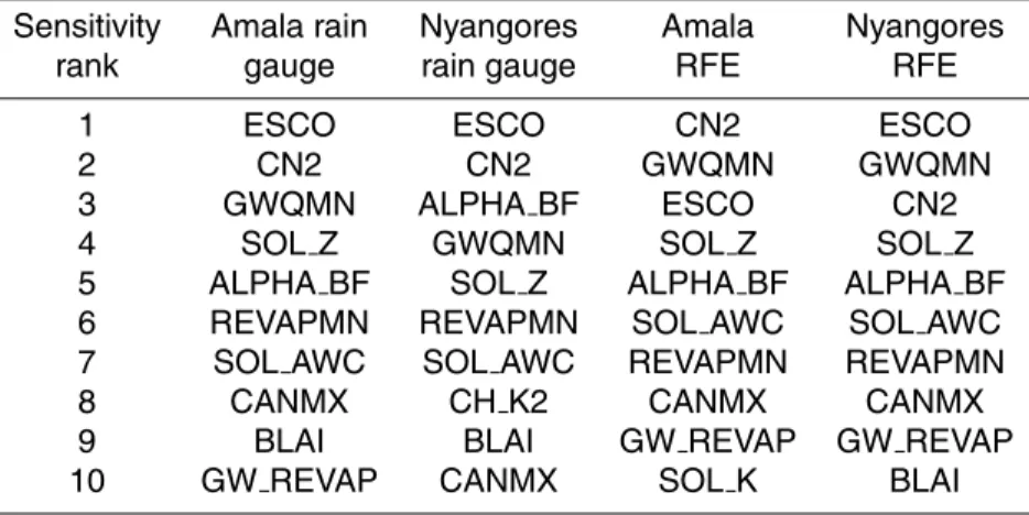
A sensitivity analysis was carried out and the 10 most sensitive parameters (Table 2)

20

were chosen for calibration of the model. The hydrological modeling exercise resulted in discharge simulation values for the Amala and Nyangores watersheds for diff er-ent rainfall inputs; Rain gauge measuremer-ents and radar rainfall estimates (RFE). The discharge hydrographs for daily and monthly data were compared for calibration and scenario analysis.

(14)

HESSD

7, 5851–5893, 2010

flux

L. M. Mango et al.

Title Page

Tables Figures

◭ ◮

Back Close

Full Screen / Esc

Discussion

P

a

per

|

Dis

cussion

P

a

per

|

Discussion

P

a

per

|

Discussio

n

P

a

per

3.2.1 Model calibration and validation

Parameter adjustment was carried out in conjunction with the statistical evaluation until an acceptable correlation or resemblance between the two datasets was achieved. Calibration is the process of estimating model parameters by comparison of model predictions or output for a given set of assumed conditions with observed or measured

5

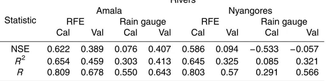
data for the same conditions (Moriasi et al., 2007). Comparison was carried out for the datasets obtained and the resulting statistics for the daily and monthly simulations are shown in the Tables 3 and 4. Statistics such as the Nash-Sutcliffe Efficiency (NSE), Pearson’s correlation coefficient (r) and the Coefficient of Correlation (R2) which were used to describe and compare the different datasets (observed and simulated).

10

In the case of the Nyangores and Amala rain gauge data models, there was a clear underperformance of the models in the case of discharge simulation as shown by the different model evaluation statistics in Moriasi et al. (2007). Calibration of the rain gauge data produced NSE values of 0.076 and−0.533 for Amala and Nyangores, re-spectively, which are considered poor. The RFE data on the other hand produced NSE

15

values of 0.622 and 0.586 for the Amala and Nyangores rivers and were considered good results.

Validation was also carried out for the model simulations and is defined as the pro-cess of demonstrating that a given site-specific model is capable of making sufficiently accurate simulations (Refsgaard, 1997). This was carried out to determine whether

20

these models were suitable for evaluating the impact of land use and climate change. For the RFE models NSE values of 0.389 and 0.094 were obtained for the Amala and Nyangores, respectively, and taking into consideration the errors that may have been introduced by missing data values, the models were considered suitable for predicting the impacts of climate and land use change. According to Abbaspour et al. (2006),

25

(15)

HESSD

7, 5851–5893, 2010

flux

L. M. Mango et al.

Title Page

Tables Figures

◭ ◮

Back Close

Full Screen / Esc

Discussion

P

a

per

|

Dis

cussion

P

a

per

|

Discussion

P

a

per

|

Discussio

n

P

a

per

|

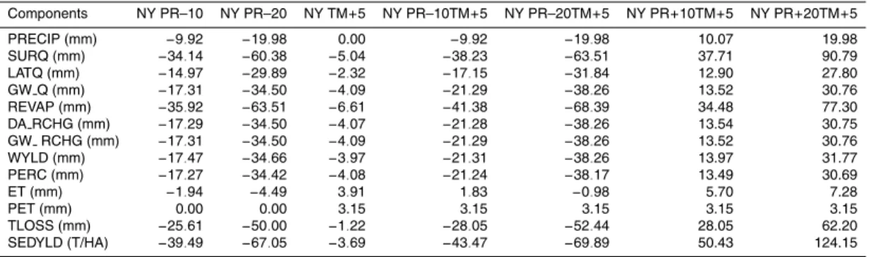
3.2.2 Climate change scenarios

Assuming accurate estimates of the water balance components, SWAT was used to evaluate the impacts of various scenarios of climate change on both the Amala and Nyangores rivers. The combined discharge hydrographs for the climate change sce-narios shown below help single out the impact a single climate change event however

5

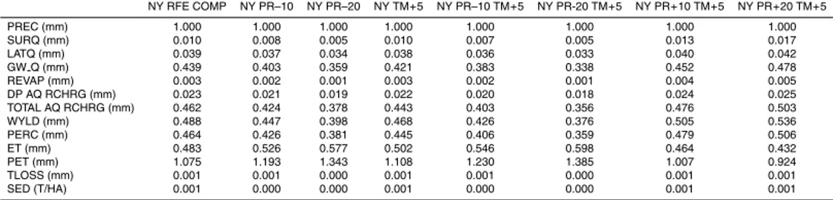
unlikely, would have on the discharge of the Nyangores river. Table 8 shows the percent changes in the annual averages of Nyangores Basin water balance components and Table 9 shows the ratio of water balance components to precipitation for these climate change scenarios.

Ogutu et al. (2007) examined the influence of the El Nino-southern Oscillation on

10

rainfall and temperature and Normalized Difference Vegetation Index fluctuations in the Mara-Serengeti ecosystem and it is anticipated that climate change will acceler-ate habitat dessication and deterioration of vegetation quality. Generally the reduction of precipitation brought about a reduction in available water in the watersheds reduc-ing baseflows to very low levels. The increase in temperature also reduces the water

15

availability to some degree by increasing evapotranspiration in the watershed thus re-ducing amount of water and discharge. According to Ficklin et al. (2009), temperature is one of the most important factors governing plant growth and depending on the op-timum temperature of the plants, the plant growth cycle will be shifted also a_ffecting the water balance components. Increases in precipitation by 10 percent and 20

per-20

cent increased the discharge and baseflow in the rivers but on the other hand may have negative e_ffects across land such as erosion and in the reach such as increased sediment load and flooding.

3.2.3 Land use change scenarios

The resulting hydrographs show the effect the different land use scenarios had on

25

(16)

HESSD

7, 5851–5893, 2010

flux

L. M. Mango et al.

Title Page

Tables Figures

◭ ◮

Back Close

Full Screen / Esc

Discussion

P

a

per

|

Dis

cussion

P

a

per

|

Discussion

P

a

per

|

Discussio

n

P

a

per

simulation. The partial deforestation and forest to agriculture scenarios resulted in high peak flows and lower baseflows while the complete deforestation scenario was characterized by high peak flows but has a baseflow that appears almost equivalent to that of the present day scenario (RFE calibrated model). Details on how these different land use scenarios a_ffected the di_fferent water balance components can be seen in

5

Table 10.

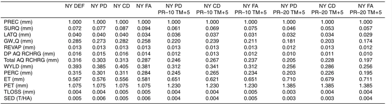
3.2.4 Combination of land use and climate change scenarios

The shown hydrographs display the discharge outputs of the land use-climate change scenarios which were more realistic scenarios in terms of future projections of land use and climate change. The most plausible land use scenarios in the case of the

Up-10

per Mara basin are the three covered in this study, with complete deforestation being the least likely to happen among the three. In the case of climate change, the most plausible are the combinations of temperature increase and precipitation increase and decrease depending on geographic location as projected by the IPCC though precipi-tation reduction is a more often occurrence in the study area as of today and therefore

15

were included in the scenarios analysis.

The resulting hydrographs and annual average for water balance components (Ta-ble 10) were a(Ta-ble to graphically show the e_ffects of the combined scenarios in terms of stream response. From the hydrographs (Figs. 7 and 8) and Fig. 10, the effect of land use on the discharge hydrographs and water balance components was evident. The

20

conversion of forest to agriculture scenario had the lowest baseflows and the cause for this is the reduction in ground water recharge which is shown in Fig. 10 and Table 10 with reductions of up to 49.99% when precipitation is reduced by 20% and a reduction of 32% when precipitation is reduced by 10% and a reduction of 48% at normal pre-cipitation. Complete deforestation on the other hand, saw an increase in surface runoff

25

(17)

HESSD

7, 5851–5893, 2010

flux

L. M. Mango et al.

Title Page

Tables Figures

◭ ◮

Back Close

Full Screen / Esc

Discussion

P

a

per

|

Dis

cussion

P

a

per

|

Discussion

P

a

per

|

Discussio

n

P

a

per

|

3.2.5 Annual average percent changes in water balance components for climate and land use-climate change scenarios

The Figs. 9 and 10 show the percent changes in the annual average water balance components for the climate and land use-climate change scenarios.

From Fig. 9, it is evident that sediment yield is the most responsive followed by revap,

5

surface runoffand transmission losses.

For the land use-climate change scenarios, the percent changes in water balance components in Fig. 10 below display the variation in the water balance components across different land uses. Details of these changes are shown in detail in Tables 10 and 11, the different land use scenarios affect the water balance components diff

er-10

ently and where these differences are most pronounced are in the surface runoffand groundwater recharge.

All the water balance components vary linearly to precipitation which can also be ob-served from the plots that are almost identical to one another especially those that are of corresponding reduction/increase in precipitation. In the land use-climate change

15

combined scenarios, there is a reduced amount of groundwater recharge, surface runoff, and total water yield to the stream meaning the water balance will be signif-icantly affected by the reduction of precipitation, increased temperature and altered land cover.

The climate change scenarios revealed that the variation of precipitation has the

20

greatest impact on the amount of discharge, sediment yield, surface runoff (a reduc-tion of 20% in precipitareduc-tion will reduce the surface runoffby half its amount in both the Amala and Nyangores watersheds) and generally to the water balance components in the watersheds. The ratio of the water balance components to precipitation reduces drastically with the reduction of precipitation. This is expected as precipitation is the

25

(18)

HESSD

7, 5851–5893, 2010

flux

L. M. Mango et al.

Title Page

Tables Figures

◭ ◮

Back Close

Full Screen / Esc

Discussion

P

a

per

|

Dis

cussion

P

a

per

|

Discussion

P

a

per

|

Discussio

n

P

a

per

Temperature increase impacts the discharge less directly than decrease in precipi-tation but nonetheless has an impact by increasing evapotranspiration and plant pro-duction which will ultimately affect land cover in the long-term. More realistic climate change simulations that combined precipitation reduction and temperature increase had the most effect on the discharge and water balance components with a reduction

5

in river discharge in both wet and dry seasons, reduction in total water yield, ground-water discharge, surface runoffand groundwater contribution to the river channel. As previous studies that have found precipitation and slope to be the main factors affecting streamflow in small watersheds, the model results show that Amala and Nyangores are no different and imply that climate change alone will have profound effects on the upper

10

Mara River flow and the human and wildlife inhabitants of the Mara River basin.

4 Conclusions

Based on the results obtained in this study, the expert classifier is a suitable methodol-ogy to classify imagery at a high and produce an accurate map of a highly variable area using far less time and effort than conventional algorithms. The resulting map obtained

15

from this land cover classification was of a high accuracy (85%) and was suitable for use as an input into SWAT especially for the simulation of effects of land use change in a spatially explicit hydrological model.

The model evaluation results (Tables 3 and 4) suggest that the calibration process may have not adequately captured the variations in the different hydrological years

20

(periods) in both the Rain gauge and RFE models which may be due to the fact that the time series data was not long enough to achieve this. In the case of the Rain gauge models compared to the RFE models, the statistics and hydrographs show the rainfall values from the Rain gauge data were not well representative of the actual rainfall that was received in the basins under study. Lack of a dense rain gauge station

25

(19)

HESSD

7, 5851–5893, 2010

flux

L. M. Mango et al.

Title Page

Tables Figures

◭ ◮

Back Close

Full Screen / Esc

Discussion

P

a

per

|

Dis

cussion

P

a

per

|

Discussion

P

a

per

|

Discussio

n

P

a

per

|

of this result. Rainfall is the main driving force of the hydrological cycle and when the rainfall for large watersheds such as the Amala and Nyangores watersheds cannot be accurately accounted for this presents a problem in the simulation process and when calibrating the model because this necessitates the rigorous adjustment of parameters which is not only a time consuming process but also may result in parameter values that

5

may give a good simulation result but are hydrologically unrealistic for the watershed. However, it can inferred that the set-up and calibration of a semi-distributed hydro-logical model such as SWAT in a large watershed with variable land cover, soils and topography is a feasible task and will yield satisfactory results given reliable data and proper attention to manual or automatic calibration.

10

The model simulations showed that the upper Mara River flow will be significantly affected in the face of the climate and land use change scenarios posing difficulties in adaptation to the altered flow regimes of the Amala and Nyangores rivers. The different water balance components were a_ffected regardless of the type and amount of change that was undergone thus affecting the magnitude and timing of the flow. It is therefore

15

prudent to work towards establishing and maintaining adequate minimum flows that would mitigate the effects of reduced baseflows and put in place measures to maintain adequate sustained river flows to the benefit of the stakeholders of the Mara River basin such as proper land and water management practices.

Acknowledgements. The authors acknowledge the Global Water for Sustainability program and

20

the United States Agency for International Development (USAID) that funded the study. Au-thors thank the Worldwide Fund for Nature Offices, Kenya and Tanzania Ministries of Water and Irrigation, and Lake Victoria South Catchment Management Authority (of Kenya’s Water Resources Management Authority). The authors thank Stefan Uhlenbrook, Delft, The Nether-lands, for reviewing this manuscript and his valuable suggestions.

(20)

HESSD

7, 5851–5893, 2010

flux

L. M. Mango et al.

Title Page

Tables Figures

◭ ◮

Back Close

Full Screen / Esc

Discussion

P

a

per

|

Dis

cussion

P

a

per

|

Discussion

P

a

per

|

Discussio

n

P

a

per

References

Abbaspour, K. C., Yang, J., Maximov, I., Siber, R., Bogner, K., Mieleitner, J., Zobrist, J., and Srinivasan, R.: Modelling hydrology and water quality in the pre-alpine/alpine Thur watershed using SWAT, J. Hydrol., 333, 413–430, 2006.

Anderson, R. J., Hardy, E. E., Roach, J. T., and Witmer, R. E.: A Land Use And Land Cover

5

Classification System For Use With Remote Sensor Data, United States Geological Survey, United States Government Printing Office, Washington D.C., 1976.

Arnold, J. G., Srinivasan, R., Muttiah, R. S., and Williams, J. R.: Large area hydrologic modeling modeling and assessment. Part I: Model development, J. Am. Water Resour. Assoc., 34, 73– 89, 1998.

10

Di Luzio, M., Srinivasan, R., and Arnold, J. G.: Integration of Watershed Tools and the SWAT Model into BASINS, J. Am. Water Resour. Assoc., 38(4), 1127–1141, 2002.

ERDAS Incorporated: ERDAS IMAGINE Tour Guides: ERDAS IMAGINE V9.3, ERDAS World-wide Headquarters, Atlanta, Georgia, pp. 662, 2006.

Ficklin, D. L., Luo, Y., Luedeling, E., and Zhang, M.: Climate change sensitivity assessment of

15

a highly agricultural watershed using SWAT, J. Hydrol., 374(2009) 16–29, 2009.

Food and Agriculture Organization (FAO) of the United Nations: Kenya Country Report, in: Irrigation in Africa in Figures, AQUASTAT Survey 2005, FAO, Rome, 2005.

Gereta, E., Wolanski, E., Borner, M., and Serneels, S.: Use of an ecohydrology model to predict the impact on the Serengeti ecosystem of deforestation, irrigation and the proposed Amala

20

Weir water Diversion Project in Kenya, Ecohydrology and Hydrobiology, 2(1–4), 135–142, 2002.

Gereta, E. and Wolanski, E.: Water quality-wildlife interaction in the Serengeti national park, Tanzania, African J. Ecol., 36(1), 1–14, 1998.

Intergovernmental Panel on Climate Change: Climate Change 2007: Synthesis Report,

Cam-25

bridge Press, Cambridge, 2007.

Jensen, J. R.: Introductory Digital Image Processing: A Remote Sensing Perspective, Third Edition, Prentice-Hall, Englewood Cliffs, New Jersey, 2005.

Liu, X. H. and Liu, Y.: The accuracy assessment in areal interpolation: An empirical investiga-tion, Sci. China Ser. E-Tech. Sci., 51, Supp. I , 62–71, 2008.

30

(21)

pre-HESSD

7, 5851–5893, 2010

flux

L. M. Mango et al.

Title Page

Tables Figures

◭ ◮

Back Close

Full Screen / Esc

Discussion

P

a

per

|

Dis

cussion

P

a

per

|

Discussion

P

a

per

|

Discussio

n

P

a

per

|

sentation at the: 8th International River Symposium, Brisbane, Australia, 6–9 September 2005.

Moriasi, D. N., Arnold, J. G., Van Liew, M. W., Bingner, R. L., Harmel, R. D., and Veith, T. L.: Model Evaluation Guidelines for Systematic Quantification of Accuracy in Watershed Simulations, Transactions of the ASABE, 50(3), 885–900, 2007.

5

Mutie, S., Mati, B., Gadain, H., and Gathenya, J.: Evaluating land use change effects on river flow using USGS geospatial stream flow model in Mara River basin, Kenya, Paper presen-tation at the 2nd Workshop of the EARSeL SIG on Land Use and Land Cover, Bonn, 28–30 September 2006.

Neitsch, S. L., Arnold, J. G., Kiniry, J. R., and Williams, J. R.: Soil and Water Assessment Tool,

10

Theoretical Documentation: Version 2005, Temple, TX. USDA Agricultural Research Service and Texas A&M Blackland Research Center, 2005.

Ogutu, O. J., Piepho, H. P., Dublin, H. T., Bhola, N., and Reid, R. S.: El Nino-Southern Oscil-lation, rainfall, temperature and Normalized Di_fference Vegetation Index Fluctuations in the Mara-Serengeti ecosystem, Afr. J. Ecol., 46, 132–143, 2007.

15

R Development Core Team: An Introduction to R: Notes on R: A Programming Environment for Data Analysis and Graphics Version 2.10.1 (2009-12-14), available online at URL http: //www.r-project.org/, 2009.

Serneels, S., Said, M. Y., and Lambin, E. F.: Land cover changes around a major east African wildlife reserve: the Mara Ecosystem (Kenya), Int. J. Remote Sens., 22(17), 3397–3420,

20

2001.

Refsgaard, J. C.: Parameterisation, calibration, and validation of distributed hydrological mod-els, J. Hydrol., 198(1), 69–97, 1997.

Setegn, S. G., Srinivasan, R., and Dargahi, B.: Hydrological Modelling in the Lake Tana Basin, Ethiopia using SWAT model, The Open Hydrology Journal, 2(2008), 25–38, 2008.

25

Survey of Kenya (SoK): National Atlas of Kenya, Fifth Edition, SoK, Nairobi, 2003.

Van der Meer, F.: Imaging spectrometry for geological applications, in: Meyers, G. R. A., En-cyclopaedia of Analytical Chemistry: Applications, Theory and Instrumentation, Wiley, New York, A2310, 31 pp., 2000.

World Resources Institute, Department of Resource Surveys and remote Sensing, Ministry of

30

(22)

Wash-HESSD

7, 5851–5893, 2010

flux

L. M. Mango et al.

Title Page

Tables Figures

◭ ◮

Back Close

Full Screen / Esc

Discussion

P

a

per

|

Dis

cussion

P

a

per

|

Discussion

P

a

per

|

Discussio

n

P

a

per

ington D.C., Nairobi, 2007.

(23)

HESSD

7, 5851–5893, 2010

flux

L. M. Mango et al.

Title Page

Tables Figures

◭ ◮

Back Close

Full Screen / Esc

Discussion

P

a

per

|

Dis

cussion

P

a

per

|

Discussion

P

a

per

|

Discussio

n

P

a

per

|

Table 1.Land use/land cover type reclassification into SWAT LU/LC classes.

Land cover type SWAT LU/LC yype

Forest Forest evergreen_{Forest deciduous}

Water Water

Bushland Forest mixed Grassland Range grasses

(24)

HESSD

7, 5851–5893, 2010

flux

L. M. Mango et al.

Title Page

Tables Figures

◭ ◮

Back Close

Full Screen / Esc

Discussion

P

a

per

|

Dis

cussion

P

a

per

|

Discussion

P

a

per

|

Discussio

n

P

a

per

Table 2.Sensitivity ranking of parameters towards water flow.

Sensitivity Amala rain Nyangores Amala Nyangores

rank gauge rain gauge RFE RFE

1 ESCO ESCO CN2 ESCO

2 CN2 CN2 GWQMN GWQMN

3 GWQMN ALPHA BF ESCO CN2

4 SOL Z GWQMN SOL Z SOL Z

5 ALPHA BF SOL Z ALPHA BF ALPHA BF

6 REVAPMN REVAPMN SOL AWC SOL AWC

7 SOL AWC SOL AWC REVAPMN REVAPMN

8 CANMX CH K2 CANMX CANMX

9 BLAI BLAI GW REVAP GW REVAP

(25)

HESSD

7, 5851–5893, 2010

flux

L. M. Mango et al.

Title Page

Tables Figures

◭ ◮

Back Close

Full Screen / Esc

Discussion

P

a

per

|

Dis

cussion

P

a

per

|

Discussion

P

a

per

|

Discussio

n

P

a

per

|

Table 3.Model evaluation statistics for daily discharge.

Statistic

Rivers

Amala Nyangores

RFE Rain gauge RFE Rain gauge

Cal Val Cal Val Cal Val Cal Val

(26)

HESSD

7, 5851–5893, 2010

flux

L. M. Mango et al.

Title Page

Tables Figures

◭ ◮

Back Close

Full Screen / Esc

Discussion

P

a

per

|

Dis

cussion

P

a

per

|

Discussion

P

a

per

|

Discussio

n

P

a

per

Table 4.Model evaluation statistics for monthly discharge.

Statistic

Rivers

Amala Nyangores

RFE Rain gauge RFE Rain gauge

Cal Val Cal Val Cal Val Cal Val

(27)

HESSD

7, 5851–5893, 2010

flux

L. M. Mango et al.

Title Page

Tables Figures

◭ ◮

Back Close

Full Screen / Esc

Discussion

P

a

per

|

Dis

cussion

P

a

per

|

Discussion

P

a

per

|

Discussio

n

P

a

per

|

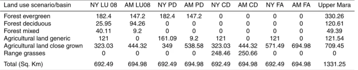
Table 5.Areal coverage of land use/land cover.

Land use scenario/basin NY LU 08 AM LU08 NY PD AM PD NY CD AM CD NY FA AM FA Upper Mara

Forest evergreen 182.4 147.2 182.4 147.2 0 0 0 0 330.26

Forest deciduous 25.95 94.26 0 0 0 0 0 0 120.61

Forest mixed 40.11 9.2 0 0 0 0 0 0 49.39

Agricultural land generic 121 0 161.09 9.2 121 0 121 0 121.54

Agricultural land close grown 323.03 444.32 349 538.58 323.03 444.32 571.49 694.98 709.45

Range grasses 0 0 0 0 248.46 250.66 0 0 0

Total (Sq. Km) 692.49 694.98 692.49 694.98 692.49 694.98 692.49 694.98 1331.25

(28)

HESSD

7, 5851–5893, 2010

flux

L. M. Mango et al.

Title Page

Tables Figures

◭ ◮

Back Close

Full Screen / Esc

Discussion

P

a

per

|

Dis

cussion

P

a

per

|

Discussion

P

a

per

|

Discussio

n

P

a

per

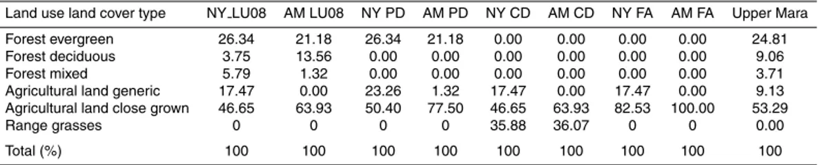
Table 6.Percent areal coverage of land use/land cover type.

Land use land cover type NY LU08 AM LU08 NY PD AM PD NY CD AM CD NY FA AM FA Upper Mara

Forest evergreen 26.34 21.18 26.34 21.18 0.00 0.00 0.00 0.00 24.81

Forest deciduous 3.75 13.56 0.00 0.00 0.00 0.00 0.00 0.00 9.06

Forest mixed 5.79 1.32 0.00 0.00 0.00 0.00 0.00 0.00 3.71

Agricultural land generic 17.47 0.00 23.26 1.32 17.47 0.00 17.47 0.00 9.13 Agricultural land close grown 46.65 63.93 50.40 77.50 46.65 63.93 82.53 100.00 53.29

Range grasses 0 0 0 0 35.88 36.07 0 0 0.00

(29)

HESSD

7, 5851–5893, 2010

flux

L. M. Mango et al.

Title Page

Tables Figures

◭ ◮

Back Close

Full Screen / Esc

Discussion

P

a

per

|

Dis

cussion

P

a

per

|

Discussion

P

a

per

|

Discussio

n

P

a

per

|

Table 7. Annual average water balance components for the calibrated Nyangores watershed models.

Components Nyangores RG 1996–2003 Nyangores RFE 2002–2008

PRECIP (mm) 1329.9 1097.2

SURQ (mm) 15.03 11.51

LATQ (mm) 60.67 43.09

GW Q (mm) 354.59 481.23

REVAP (mm) 21.89 3.48

DA RCHG (mm) 22.47 25.33

GW RCHG (mm) 449.43 506.63

WYLD (mm) 429.28 535

PERC (mm) 450.02 509.52

ET (mm) 789 530

PET (mm) 1150.3 1179

TLOSS (mm) 1.01 0.82

SEDYLD (T/HA) 0.686 0.704

(30)

HESSD

7, 5851–5893, 2010

flux

L. M. Mango et al.

Title Page

Tables Figures

◭ ◮

Back Close

Full Screen / Esc

Discussion

P

a

per

|

Dis

cussion

P

a

per

|

Discussion

P

a

per

|

Discussio

n

P

a

per

Table 8. Percent changes in the annual averages of Nyangores Basin water balance compo-nents for climate change scenarios.

Components NY PR–10 NY PR–20 NY TM+5 NY PR–10TM+5 NY PR–20TM+5 NY PR+10TM+5 NY PR+20TM+5

PRECIP (mm) −9.92 −19.98 0.00 −9.92 −19.98 10.07 19.98

SURQ (mm) −34.14 −60.38 −5.04 −38.23 −63.51 37.71 90.79

LATQ (mm) −14.97 −29.89 −2.32 −17.15 −31.84 12.90 27.80

GW Q (mm) −17.31 −34.50 −4.09 −21.29 −38.26 13.52 30.76

REVAP (mm) −35.92 −63.51 −6.61 −41.38 −68.39 34.48 77.30

DA RCHG (mm) −17.29 −34.50 −4.07 −21.28 −38.26 13.54 30.75

GW RCHG (mm) −17.31 −34.50 −4.09 −21.29 −38.26 13.52 30.76

WYLD (mm) −17.47 −34.66 −3.97 −21.31 −38.26 13.97 31.77

PERC (mm) −17.27 −34.42 −4.08 −21.24 −38.17 13.49 30.69

ET (mm) −1.94 −4.49 3.91 1.83 −0.98 5.70 7.28

PET (mm) 0.00 0.00 3.15 3.15 3.15 3.15 3.15

TLOSS (mm) −25.61 −50.00 −1.22 −28.05 −52.44 28.05 62.20

(31)

HESSD

7, 5851–5893, 2010

flux

L. M. Mango et al.

Title Page

Tables Figures

◭ ◮

Back Close

Full Screen / Esc

Discussion

P

a

per

|

Dis

cussion

P

a

per

|

Discussion

P

a

per

|

Discussio

n

P

a

per

|

Table 9. Ratio of water balance components to precipitation for the Nyangores Basin climate change scenarios.

NY RFE COMP NY PR–10 NY PR–20 NY TM+5 NY PR–10 TM+5 NY PR-20 TM+5 NY PR+10 TM+5 NY PR+20 TM+5 PREC (mm) 1.000 1.000 1.000 1.000 1.000 1.000 1.000 1.000 SURQ (mm) 0.010 0.008 0.005 0.010 0.007 0.005 0.013 0.017 LATQ (mm) 0.039 0.037 0.034 0.038 0.036 0.033 0.040 0.042 GW Q (mm) 0.439 0.403 0.359 0.421 0.383 0.338 0.452 0.478 REVAP (mm) 0.003 0.002 0.001 0.003 0.002 0.001 0.004 0.005 DP AQ RCHRG (mm) 0.023 0.021 0.019 0.022 0.020 0.018 0.024 0.025 TOTAL AQ RCHRG (mm) 0.462 0.424 0.378 0.443 0.403 0.356 0.476 0.503 WYLD (mm) 0.488 0.447 0.398 0.468 0.426 0.376 0.505 0.536 PERC (mm) 0.464 0.426 0.381 0.445 0.406 0.359 0.479 0.506 ET (mm) 0.483 0.526 0.577 0.502 0.546 0.598 0.464 0.432 PET (mm) 1.075 1.193 1.343 1.108 1.230 1.385 1.007 0.924 TLOSS (mm) 0.001 0.001 0.000 0.001 0.001 0.000 0.001 0.001 SED (T/HA) 0.001 0.000 0.000 0.001 0.000 0.000 0.001 0.001

(32)

HESSD

7, 5851–5893, 2010

flux

L. M. Mango et al.

Title Page

Tables Figures

◭ ◮

Back Close

Full Screen / Esc

Discussion

P

a

per

|

Dis

cussion

P

a

per

|

Discussion

P

a

per

|

Discussio

n

P

a

per

Table 10.Percent changes in the annual averages of Nyangores Basin water balance compo-nents for land use-climate change scenarios.

C NY PD NY CD NY FA NY PD NY PD NY CD NY CD NY FA NY FA

PR–10 TM+5 PR–20 TM+5 PR–10 TM+5 PR–20 TM+5 PR–10TM+5 PR–20 TM+5 PRECIP (mm) 0.00 −9.92 −19.98 0.00 −9.92 −19.98 0.00 −9.92 −19.98 SURQ (mm) 6.94 −24.08 −48.85 20.58 −13.61 −41.47 31.49 −5.99 −36.31 LATQ (mm) −1.56 −20.65 −35.94 −0.66 −17.55 −32.60 −14.91 −30.31 −43.44 GW Q (mm) −4.16 −30.49 −49.05 −0.75 −24.38 −43.01 −9.39 −33.28 −51.00 REVAP (mm) −1.84 −12.76 −26.76 −0.89 −10.03 −23.28 −2.80 −12.76 −27.37 DA RCHG (mm) −4.04 −29.68 −48.09 −0.75 −23.79 −42.21 −9.06 −32.33 −50.00 GW RCHG (mm) −4.06 −29.71 −48.12 −0.79 −23.78 −42.21 −9.09 −32.35 −49.99 WYLD (mm) −2.00 −28.50 −47.85 2.93 −21.96 −41.88 −3.00 −28.49 −47.98 PERC (mm) −4.22 −29.92 −48.36 −1.10 −24.07 −42.49 −9.71 −32.91 −50.50 ET (mm) 1.64 3.46 0.23 −1.93 −1.33 −4.20 2.46 3.50 0.35

PET (mm) 0.00 3.15 3.15 0.00 3.15 3.15 0.00 3.15 3.15

TLOSS (mm) 9.90 −10.15 −29.21 23.76 1.49 −19.80 45.30 20.30 −4.46 SEDYLD (T/HA) 22.39 −12.37 −42.73 11.90 −22.78 −50.15 41.48 1.19 −33.21

(33)

HESSD

7, 5851–5893, 2010

flux

L. M. Mango et al.

Title Page

Tables Figures

◭ ◮

Back Close

Full Screen / Esc

Discussion

P

a

per

|

Dis

cussion

P

a

per

|

Discussion

P

a

per

|

Discussio

n

P

a

per

|

Table 11. Ratio of water balance components to precipitation for the Nyangores Basin land use-climate change scenarios.

(34)

HESSD

7, 5851–5893, 2010

flux

L. M. Mango et al.

Title Page

Tables Figures

◭ ◮

Back Close

Full Screen / Esc

Discussion

P

a

per

|

Dis

cussion

P

a

per

|

Discussion

P

a

per

|

Discussio

n

P

a

per

(35)

HESSD

7, 5851–5893, 2010

flux

L. M. Mango et al.

Title Page

Tables Figures

◭ ◮

Back Close

Full Screen / Esc

Discussion

P

a

per

|

Dis

cussion

P

a

per

|

Discussion

P

a

per

|

Discussio

n

P

a

per

|

(36)

HESSD

7, 5851–5893, 2010

flux

L. M. Mango et al.

Title Page

Tables Figures

◭ ◮

Back Close

Full Screen / Esc

Discussion

P

a

per

|

Dis

cussion

P

a

per

|

Discussion

P

a

per

|

Discussio

n

P

a

per

(37)

HESSD

7, 5851–5893, 2010

flux

L. M. Mango et al.

Title Page

Tables Figures

◭ ◮

Back Close

Full Screen / Esc

Discussion

P

a

per

|

Dis

cussion

P

a

per

|

Discussion

P

a

per

|

Discussio

n

P

a

per

|

(38)

HESSD

7, 5851–5893, 2010

flux

L. M. Mango et al.

Title Page

Tables Figures

◭ ◮

Back Close

Full Screen / Esc

Discussion

P

a

per

|

Dis

cussion

P

a

per

|

Discussion

P

a

per

|

Discussio

n

P

a

per