www.hydrol-earth-syst-sci.net/16/473/2012/ doi:10.5194/hess-16-473-2012
© Author(s) 2012. CC Attribution 3.0 License.
Earth System
Sciences
Investigating riparian groundwater flow close to a losing river using
diurnal temperature oscillations at high vertical resolution
T. Vogt1,*, **, M. Schirmer1, and O. A. Cirpka2
1Eawag – Swiss Federal Institute of Aquatic Science and Technology, ¨Uberlandstr. 133, 8600 D¨ubendorf, Switzerland 2University of T¨ubingen, Center for Applied Geoscience, Sigwartstr. 10, 72076 T¨ubingen, Germany
*now at: Nagra, National Cooperative for the Disposal of Radioactive Waste, Hardstrasse 73, 5430 Wettingen, Switzerland **Invited contribution by T. Vogt, recipient of the Outstanding Student Poster Award 2009.
Correspondence to:M. Schirmer (mario.schirmer@eawag.ch)
Received: 6 June 2011 – Published in Hydrol. Earth Syst. Sci. Discuss.: 29 June 2011 Revised: 7 January 2012 – Accepted: 29 January 2012 – Published: 14 February 2012
Abstract. River-water infiltration is of high relevance for hyporheic and riparian groundwater ecology as well as for drinking water supply by river-bank filtration. Heat has come a popular natural tracer to estimate exchange rates be-tween rivers and groundwater. However, quantifying flow patterns and velocities is impeded by spatial and temporal variations of exchange fluxes, insufficient sensors spacing during field investigations, or simplifying assumptions for analysis or modeling such as uniform flow. The objective of this study is to investigate lateral shallow groundwater flow upon river-water infiltration at the shoreline of the riverbed and in the adjacent riparian zone of the River Thur in north-east Switzerland. Here we have applied distributed tempera-ture sensing (DTS) along optical fibers wrapped around tubes to measure high-resolution vertical temperature profiles of the unsaturated zone and shallow riparian groundwater. Di-urnal temperature oscillations were tracked in the subsurface and analyzed by means of dynamic harmonic regression to extract amplitudes and phase angles. Subsequent calcula-tions of amplitude attenuation and time shift relative to the river signal show in detail vertical and temporal variations of heat transport in shallow riparian groundwater. In addition, we apply a numerical two-dimensional heat transport model for the unsaturated zone and shallow groundwater to obtain a better understanding of the observed heat transport processes in shallow riparian groundwater and to estimate the ground-water flow velocity. Our results show that the observed ri-parian groundwater temperature distribution cannot be de-scribed by uniform flow, but rather by horizontal ground-water flow velocities varying over depth. In addition, heat transfer of diurnal temperature oscillations from the losing
river through shallow groundwater is influenced by thermal exchange with the unsaturated zone. Neglecting the influ-ence of the unsaturated zone would cause biased interpre-tation and underestimation of groundwater flow velocities. The combination of high resolution field data and modeling shows the complex hydraulic and thermal processes occur-ring in shallow riparian groundwater close to losing river sections as well as potential errors sources for interpreting diurnal temperature oscillations in such environments.
1 Introduction
flow through small-scale bedforms, is of minor relevance. For groundwater questions, the key quantities of interest are the net water flux from the river into the aquifer, or vice versa, and the travel time distribution of solutes within the riparian zone. While net exchange fluxes on the length scales of river reaches are typically estimated by calibrat-ing regional-scale groundwater models, the determination of travel times requires groundwater observations within the riparian zone close to rivers. These observations are of-ten restricted to single point measurements in observation wells, so that information about spatial variability and thus the representativeness of the observations is missing.
In recent years, temperature fluctuations have increasingly been used as a natural tracer for investigations of hyporheic exchange and groundwater travel times (Fanelli and Lautz, 2008; Goto et al., 2005; Schmidt et al., 2006; Hoehn and Cirpka, 2006; Su et al., 2004). In contrast to artificial tracer tests for the determination of travel times and flow veloci-ties upon bank filtration, the temperature fluctuations of river water offer a natural, continuous varying signal that can be measured in a cost-efficient and robust way. Recently, An-derson (2005) and Constantz (2008) reviewed how heat can be utilized as a tracer for hydrological purposes, where seep-age rates in riverbeds and travel times in the riparian zone are calculated based on temperature profiles and time se-ries. In this context, quasi-transient analytical solutions of one-dimensional (1-D) heat transport with sinusoidal fluctu-ations of heat-input from the top and constant groundwater temperature at bottom are most commonly applied (Silliman et al., 1995; Stallman, 1965). Based on this approach, sev-eral methods of time-series analysis have been developed to calculate time-dependent streambed seepage rates using ex-tracted amplitudes and time shifts of the diurnal tempera-ture signal (Gordon et al., 2012; Hatch et al., 2006; Keery et al., 2007; Vogt et al., 2010b). For short travel times in the hyporheic zone of the riverbed, or in riparian groundwa-ter close to the river, diurnal temperature oscillations are the common signal of choice, because the high frequency allows short monitoring periods in the range of single days to weeks. As high-frequency temperature fluctuations are lost due to strong dampening within a few meters of travel distance, the travel time from a losing river to a near-by pumping well may be inferred from the seasonal rather than diurnal temperature signal (Sheets et al., 2002; Vogt et al., 2009), requiring longer monitoring periods and neglecting dynamics on time scales of weeks and smaller.
Thermal sediment properties needed for the analysis of heat transport in porous media are less variable than hy-draulic sediment properties, which is an advantage of heat as tracer over Darcy based methods. However, simplify-ing assumptions, commonly made in the analysis of heat as a tracer, may lead to systematic errors in the interpre-tation. Lautz (2010) showed that non-uniform flow causes the biggest error in 1-D velocity estimates compared to other non-ideal field conditions, such as a non-sinusoidal signal
and a thermal gradient. In addition, uncertainty in thermal diffusivity, sensor spacing, and the accuracy of temperature sensors can cause erroneous predictions of seepage ties, especially for gaining conditions and low flow veloci-ties (Shanafield et al., 2011). Rau et al. (2010) tested the advantages, limitations and applicability of the methods of Hatch et al. (2006) and Stallman (1965). They hypothesized that analyzing temperature profiles and time series caused by multi-dimensional flow using 1-D solutions may result in inaccurate estimates and that the conditions of a repre-sentative elementary volume (REV) needed in the analysis may not be satisfied at the scale of investigation. Molina-Giraldo et al. (2011) demonstrated in a modeling study that conductive heat transfer between shallow aquifers, the un-derlying aquitard, and the overlaying unsaturated zone may significantly influence transport of seasonal temperature sig-nals through groundwater, and neglecting these impact could cause severe errors in the estimates of groundwater velocity from these signals.
authors confirmed that wrapped DTS measurement systems provide a reliable method to monitor temperature in space and time.
Whereas the temporal and spatial variability of hyporheic exchange in riverbeds has repeatedly been studied on differ-ent scales (K¨aser et al., 2009; Wroblicky et al., 1998), the vertical variability of horizontal riparian groundwater flow upon bank-filtration is widely unproved by field data. This has consequences in the interpretation of single-point tem-perature time series for the assessment of bank filtration. Likewise, classical 1-D interpretation of temperature time series neglecting transverse heat conduction may cause a systematic bias in estimated travel times. Molina-Giraldo et al. (2011) showed that seasonal temperature signals are severely modified by vertical conductive heat transfer be-tween the aquifer and the underlying aquitard and the over-laying unsaturated zone, respectively. Because diurnal sig-nals are attenuated over shorter travel distances than seasonal ones, the significance of heat conduction on overall transfer of the periodic temperature signals may be smaller. However, field data have not been analyzed in this regard.
The objective of this study is to investigate heat transport upon river-water infiltration at the shoreline of the riverbed and in the adjacent riparian zone of the losing River Thur in northeast Switzerland by means of diurnal temperature os-cillations at high vertical resolution. These profiles may be modified by vertical variation of groundwater flow and con-ductive heat exchange with the unsaturated zone. We want to estimate these influences and examine the error that would be introduced if we interpreted single-point diurnal temper-ature time series by the classical 1-D heat-transport model with uniform coefficients neglecting heat exchange with the unsaturated zone. Towards this end, we use time series of three high-resolution fiber-optic temperature profiles (verti-cal resolution = 5 mm) in the riverbed, at the shoreline of the river, and in the riparian zone. The time-dependent amplitude dampening and time shift of the diurnal signal in the sedi-ments with respect to the river signal is calculated by means of dynamic harmonic regression (Young et al., 1999). In ad-dition, we simulate two-dimensional heat transport in a verti-cal cross-section covering the saturated and unsaturated zone to estimate groundwater flow velocities and to demonstrate how transport of diurnal temperature signals within shallow groundwater in the river bank is affected by heat exchange with the unsaturated zone.
2 Theory
2.1 Heat transport equation in time and spectral domains
Heat transport in porous media can be described by the convection-conduction equation (Domenico
and Schwartz, 2008):
∂T
∂t +vT· ∇T− ∇ ·(DT∇T )=0 (1)
with: vT=
ρwCw
ρsCs(1−n)+ρwCwn q;DT
=λ 1−n
s λ
nSw
w λgn(1−Sw)I+ρwCwDdisp
ρsCs(1−n)+ρwCwnSw
, (2)
in whichT denotes temperature (K),tis time (s),vT is the ef-fective velocity of convective heat transport (m s−1), andDT is the effective diffusivity tensor for heat transfer (m2s−1).
ρw,Cw, andλware the mass density (kg m−3), specific heat capacity (J kg K−1), and thermal conductivity (W m−1K−1) of water. ρs, Cs, and λs are the corresponding properties of the solids;λg is the thermal conductivity (W m K−1) of gas;n denotes porosity;Sw is the water saturation (-); and I is the identity matrix. The bulk thermal conductivity is approximated by the volume-weighted geometric average of the water-, gas-, and solid-phase thermal conductivities. The heat capacity of soil gas is neglected. The effective thermal velocity depends onq, which is the specific discharge vector, and the thermal diffusivity is related toDdisp, which is the hydrodynamic dispersion tensor.
We use the van-Genuchten/Mualem parameterization to estimate the water saturationSwin the unsaturated zone (van Genuchten, 1980):
Sw=
1+(αhc)N 1−NN
, (3)
in whichα(1/m) andN (-) are the van-Genuchten parame-ters, andhcis the capillary head (m), which may be approxi-mated as the distance to the groundwater table for hydrostatic conditions in the unsaturated zone.
In the following review of analytical results, we assume that the transport coefficientsvT andDT are constant, facil-itating convenient transformation of the heat-transport equa-tion into the spectral domain. The Fourier transformT (f,˜ x)
ofT (t,x) in time is defined as: ˜
T (f,x)=
Z ∞ −∞
T (t,x)exp(−2π itf )dt , (4) in which f is the frequency (1/s), and i is the imaginary number. Then, the heat-transport equation 2 becomes in the spectral domain:
2π ifT˜+vT· ∇ ˜T− ∇ ·(DT∇ ˜T )=0, (5) subject to Fourier-transformed boundary conditions. 2.2 Analytical solution of one-dimensional heat
transport equation
with constant coefficients (Stallman, 1965). Here we set a fixed, time-periodic temperature at the bottom of the stream, with distance z= 0, and vanishing fluctuations at the limit
z→ ∞as boundary conditions:
T (z=0,t )= ¯T0+a0×cos(2π(t−t0max)f ) lim
z→∞T (z,t )= ¯T∞
, (6)
in whichT0andT∞ are the mean temperatures (K) in the
river and the aquifer at infinite distance from the stream bot-tom, respectively,a0is the amplitude (K) of temperature fluc-tuations in the river, andtmax is the time (s) of maximum temperature in the river. In the spectral domain, the analyt-ical solution is an exponential function ofz with complex exponent. Transformation into the time-domain yields (Stall-man, 1965):
T (z,t )= ¯T0+a0×exp
−z
zp
×cos2πt−t0max−z
c
f, (7) in which c and zp are the frequency-dependent celerity (m s−1) and penetration distance (m) of temperature propagation.
c=vT v u u t1 2+ 1 2 s
1+64π 2f2D2
T
vT4 ; (8)
zp= 2DT
c−vT
. (9)
2.3 Dynamic harmonic regression
To extract the diurnal sinusoidal components from the tem-perature time series, we use dynamic harmonic regression (Young et al., 1999) as presented by Kerry et al. (2007) and Vogt et al. (2010b). This non-stationary extension of Fourier analysis is implemented in the Matlab-based captain toolbox (Taylor et al., 2007). The forward model is similar to the standard spectral representation of the time series:
T (t )=a0(t )+
nf
X
i=1
αi(t )cos
2π it
τ
+βi(t )sin
2π it
τ
, (10) in whicha0(t )is the trend, whereasαi(t )andβi(t )are the sine and cosine contributions of the frequencyi/τ, in which
τ is the base period (here one day). All time-dependent co-efficients are assumed to be auto-correlated in time. For a detailed description of the determination ofα0(t ),αi(t )and
βi(t )we refer to Young et al. (1999) and Taylor et al. (2007). From the sine and cosine coefficients αi(t ) and βi(t ) the time-dependent amplitude ai(t ) and phase angle φi(t ) for frequencyi/τ at timetare calculated:
ai(t )= q
αi2(t )+βi2(t ); (11)
ϕi(t )=tan−1 α
i(t )
βi(t )
. (12)
We convert the resulting phase anglesφ(z,t,f )of the diurnal signal for each time pointt and distancezto a time point of maximum temperaturetmax:
tmax(z,t,f )= −ϕ(z,t,f )
2πf . (13)
Then, the time shifttshift(z,t,f )between the diurnal river and groundwater signals is iteratively calculated by:
tshift(z,t,f )=tmax(z,t,f )−tmax(0,t−tshift(z,t,f ),f ). (14) In addition, we compute the attenuation of the diurnal river temperature signal A(z,t,f ) during transport through the riverbed to the riparian zone at each time pointtand distance
z:
A(z,t,f )=ln a river
i (t−tshift(z,t,f ),f )
ai(z,t,f )
!
. (15) For a time-constant observation distancezwe determine the apparent effective velocityvT(z,t,f )and the apparent effec-tive diffusivityDT(z,t,f )of temperature transport after Vogt et al. (2010b) based on the attenuation A(z, t, f ) and the apparent celerityc(z,t,f )of the diurnal temperature signal:
c(z,t,f )= z
tshift(z,t,f )
, (16)
W (vT,DT)= 1−
vT c v u u t1 2+ 1 2 s
1+64π 2f2D2
T
vT4
2 +
1− 2ADT
(c−vT)z 2
, (17)
in which we have dropped the argument (z,t,f )for conve-nience. Thereto, the sum of the squared relative residuals of
c(vT,DT,f )andzp(vT,DT,f )is minimized and optimiza-tion is done by the Nelder-Mead simplex algorithm that is implemented in the Matlab function fminsearch (Lagarias et al., 1998). Finally, the apparent Darcy velocityq(z,t )related to the diurnal temperature signal (f= 1/day) is estimated, if
zis known and constant over time:
q(z,t )=vT(z,t,f )
ρsCs(1−n)+ρwCwn
ρwCw
. (18)
3 Field site
Fig. 1.Thur catchment and location of the field site at the restored river section Niederneunforn/Altikon.
the headwaters cause short but rapid increases of discharge. Mean annual precipitation of the field site area is 908 mm and average monthly temperatures range from 0.9◦C in January to 19.0◦C in July (https://gate.meteoswiss.ch/idaweb).
The aquifer in the Thur valley consists of Pleistocene glacio-fluvial sandy gravels overlaying impervious lacustrine clays. Alluvial fines of up to 2 m thickness act as a confin-ing layer on top of the aquifer, which is 5–7 m thick and has a hydraulic conductivity of≈3×10⁻³m s−1(Schneider et al., 2011). During low flow, the aquifer is largely uncon-fined, but it turns confined during higher river stage. The riverbed consists of sandy gravel and is hydraulically well connected to the aquifer. At the field site, the major ground-water recharge originates from continuous river-ground-water infil-tration into the aquifer (Vogt et al., 2010a). The infilinfil-tration velocity in the restored riverbed was estimated to fluctuate in the range of 1.5×10⁻⁵m s−1to 4.5×10⁻⁵m s−1(Vogt et al., 2010b).
The field site is located at a restored section of River Thur and has been detailed investigated by the RECORD project (Assessment and Modeling of Coupled Ecological and Hy-drological Dynamics in the Restored Corridor of a River (Re-stored Corridor Dynamics; http://www.cces.ethz.ch/projects/ nature/Record)). Here, the restored riverbed is 60–100 m wide and shows distinct riverbed morphology. The north-ern bank stabilization has been removed resulting in a ripar-ian zone with a natural succession of bare gravel, grass col-onized gravel, willow belt and alluvial forest. Field instal-lations consist of a river gauging station, observation wells with integrated water-level, temperature, and electrical con-ductivity sensors, meteorological stations and soil sensors, among others (Schneider et al., 2011).
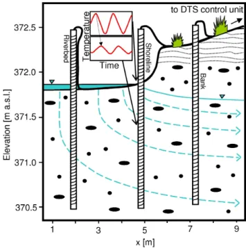
Fig. 2. Sketch of the experimental set-up in the field. During low river stage the top sediments of the fiber-optic high-resolution pro-filer at the shoreline were unsaturated. In the following temperature data of the shoreline and bank are discussed in detail.
4 Methods
4.1 Fiber-optic high-resolution temperature profiling
made by a steel-protected fiber-optic cable (Drahtex Arma Fiber) of which 5–10 m were stored in a box filled with a water-ice mixture for calibration. We monitored the tem-perature in the ice bath, the river water and air temtem-perature with Onset TidbiT v2 sensors (0.02 K resolution, 0.2 K accu-racy). The DTS data of each wrapped optical fiber showed a different temperature offset and systematic drift and were corrected by comparison with the TidBit data.
For field installation of the fiber-optic high-resolution temperature profilers we used a direct-push machine that pushed 3.25 inch metal rods with an expandable tip into the sediments. The wrapped tubes fit into the metal rods (ID = 67 mm) of the direct-push system and remain with the expendable tip in the ground after pulling the outer metal rod. We installed one of the three high-resolution tempera-ture profilers in the riverbed, one at the shoreline, and one in the riparian bank along a presumed subsurface flow path (Fig. 2). The investigated area is about 40 m upstream of the experiment of Vogt et al. (2010b) on the northern side of the restored river section. Here, the riverbed has an eleva-tion of 371.8 m a.s.l. and the elevaeleva-tion of the bank is about 372.3 m a.s.l. (Fig. 2). The installation depth of the lower end of the wrapped fibers was 370.5 m a.s.l., but the num-ber of measuring points in air, river-water, saturated and unsaturated zone varied depending on the location and on water-level (Fig. 2). The presented data were acquired during 22 days in September 2010.
4.2 Numerical heat-transport model
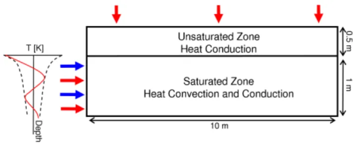
We modified the 2-D spectral finite element model of Molina-Giraldo et al. (2011) to simulate heat transport of di-urnal temperature oscillations within a vertical cross section, mimicking the conditions at the experimental site. The sim-plified model is applied to the field conditions during the end of the field observation period when groundwater head was relatively stable and no precipitation occurred. The model accounts for conductive/dispersive and convective heat trans-fer in a steady-state groundwater flow field, conductive heat transfer through the unsaturated zone on top, and diurnal temperature fluctuations at the shoreline of the riverbed as well as at the land surface of the river bank (Fig. 3).
The model consists of two layers representing the unsat-urated and satunsat-urated zone of the riparian zone. The thick-ness of the unsaturated zone is set to 0.5 m and that of the aquifer to 1 m, mimicking the experimental set-up of the high-resolution temperature profiler in the bank (see Fig. 2). The horizontal extension of the model domain is 10 m. The uniform grid has a vertical resolution of 0.01 m and a hor-izontal resolution of 0.02 m. A no-flow boundary condi-tion is applied to the bottom of the domain. The water en-ters the aquifer on the left side with horizontal flow and leaves the aquifer through the right side. The flow field is strictly horizontal and computed analytically. We start with a uniform velocity distribution over the entire aquifer
thick-Fig. 3. Set-up of the numerical 2-D heat transport model. Blue arrows indicate horizontal groundwater inflow, red arrows indicate periodic heat input. For the periodic heat input on the left side of the aquifer observed amplitude and time-shift profiles of the high-resolution pole at the shoreline are converted into temperature fluc-tuations.
ness. However, velocities can be adjusted to obtain horizon-tal groundwater flow velocities varying over depth. We con-sider horizontal flow in the unsaturated zone by multiplying the groundwater-related specific discharge with the relative permeability according to the van Genuchten (1980) param-eterization. Recharge through the unsaturated zone caused by precipitation or river flooding can be added to the simula-tions, but was not necessary as no precipitation was observed during the end of the field observation period.
At the land surface, the temperature oscillations are simu-lated by a frequency of 1/day and a constant amplitude of 6 K, which is shifted from the river signal as observed at the bank temperature profiler. The amplitude of 6 K refers to the observed air temperature between 21 September and 23 September 2010. At the left-hand boundary of the ground-water layer we used amplitude and time-shift profiles of the high-resolution temperature profiler installed at the shoreline from 22 September 2010 at 00:08 CEST as boundary condi-tion. The data were converted into temperature fluctuations. For the unsaturated part of the left- and right-hand bound-aries and for the bottom boundary, we assumed zero heat flux. Heat flux at the right aquifer boundary is restricted to convection. The thermal and hydraulic parameters used in the model are literature values typical for sandy gravel sediments consisting of a quartz-calcite mixture (Table 1).
The model simulates the 2-D distribution of Fourier trans-formed temperature fluctuations T (f,˜ x). The amplitude
aT (K) and phase shift φT (s) of the simulated diurnal temperature signal is then given by:
aT = T˜
; (19)
ϕT =tan−1
Re(T )˜ I m(T )˜
, (20)
Table 1.Thermal and hydraulic properties after Sch¨on (1998) and de Marsily (1986) used for analysis and modeling. N and αare the van Genuchten parameters for sandy loam after Carsel and Par-rish (1988).
Density of water (kg m−3) 1000
Density of solids (kg m−3) 2680
Specific heat capacity of water (J kg−1K−1) 4190 Specific heat capacity of solids (J kg−1K−1) 733 Heat conductivity of water (W m−1K−1) 0.58 Heat conductivity of solids (W m−1K−1) 4.47 Thermal conductivity of gas phase (W m−1K−1) 0.025
Porosity (–) 0.25
Longitudinal dispersivity (m) 0.1
Transverse dispersivity (m) 0.001
Specific discharge of aquifer
for uniform flow (m s−1) 6.9×10⁻⁵
Specific discharge of aquifer
for depth variable flow (m s−1) 5.8–10.4×10⁻⁵
α(1/m) 5
N 1.4
5 Results
5.1 Temperature distribution
During the monitoring period, the river water had a mean temperature of 14.6◦C with diurnal amplitudes of 0.4– 2.3◦C. The mean air temperature was identical, but diurnal amplitudes were in average 2.3 times higher. Throughout the measurement campaign several minor storm events oc-curred resulting in higher river stage (at 2, 9, and 13 Septem-ber 2010). We stopped monitoring on 25 SeptemSeptem-ber when a big storm event followed by a major flood occurred. Al-though the experimental set-up was designed for temporary use, the installations were fully operational after major flood events. Manual measurements of the water table at the three profilers agree well with extrapolated water level data of a well close to the river, where a pressure sensor was installed. The temperature data of the fiber-optic high-resolution temperature profiler in the riverbed were analyzed after Vogt et al. (2010b). The calculated seepage rates range between 0.6–1.0×10⁻⁵m s−1 in 0.2 m and in 0.6–0.7 m depth be-low the riverbed and between 1.0–3.0×10⁻⁵m s−1 in 0.2– 0.6 m depth. In the following, we focus on the shoreline and the bank where an unsaturated zone exists and horizontal flow is dominant.
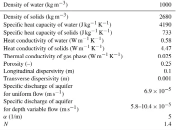
The upper part of the high-resolution fiber-optic temper-ature profiler at the shoreline lay above the sediments and the rest in the sandy gravel sediments (Fig. 4a). In contrast to the profiler in the riverbed, an unsaturated zone of up to 0.15 m existed at the shoreline under low flow conditions. During higher river stage, the sediments were flooded. A sharp temperature contrast illustrates the interfaces between
air and river water as well as air and sediments (Fig. 4a). The high-resolution fiber-optic temperature profiler in the bank had only a small wrapped section exposed to the air. Figure 4b shows the temperature data of the wrapped op-tical fiber which was installed in the bank sediments with-out air temperature. Here, the top sediment layer consists of silty fine sand with a thickness of about 0.2 m overlaying the sandy-gravel aquifer. Until the end of the monitoring cam-paign, when the major flood occurred, an unsaturated zone with varying thickness of 0.25–0.60 m existed in the bank.
In the deepest 0.2–0.3 m of the 1.93 m long wrapped section, the DTS noise (standard deviation of the ice bath = 0.2 K) exceeded the very small diurnal temperature os-cillations (amplitudes<0.05 K). Therefore, we focus on the temperature distribution from above 370.7 m a.s.l. to the land surface. The data of the high-resolution temperature profil-ers reveal in detail the temperature distribution in riparian groundwater over depth and time. The unsaturated sediments are characterized by the strongest oscillations, whereas the lower groundwater shows the lowest diurnal temperature os-cillations. The heat signal at the land surface propagates into the unsaturated zone. If the distance to groundwater is low, like at the shoreline, the maximum penetration depth lies below the water table (Fig. 4c). In the riparian bank, the signal of the land surface is strongly damped in the top sediments and disappears before reaching the groundwater table (Fig. 4d). The signals of river and land surface tem-perature interfere at the shoreline in shallow groundwater, whereas the middle and deeper groundwater temperatures are apparently determined by the river signal only (Fig. 4c). In the riparian bank the groundwater temperature seems to in-fluence the deepest part of the unsaturated zone where the signal of the land surface is completely damped, indicating conductive heat exchange between groundwater and unsatu-rated zone. In groundwater, the temperature pattern shows slightly curved features that disappear below 370.7 m a.s.l. The curved shape of vertical groundwater temperature distri-bution is more pronounced in the bank than at the shoreline of the riverbed and originates from the earlier occurrence of the temperature maximum in the middle part of groundwa-ter compared to shallow and deeper groundwagroundwa-ter (Fig. 4d). Due to the high resolution, the temporal and spatial vari-ability of the penetration depths of the river and land sur-face signals as well as their interference is visible in the temperature distributions.
5.2 Results of dynamic harmonic regression analysis
Fig. 4.Temperature distribution along the fiber-optic temperature profilers. The black solid line indicates the water level.(A)Shoreline. The white solid line indicates the top of the sediments. The presence of an unsaturated zone depends on the river stage.(B)Riparian bank. The top of the figure marks the land surface. During the monitoring period the thickness of the unsaturated zone varied between 0.25–0.60 m.
(C)Detailed temperature distribution of the sediments at the shoreline.(D)Detailed temperature distribution in the riparian bank.
attenuation and time shift of the diurnal signal in groundwa-ter related to the river temperature. Although the ground-water temperature might be influenced by the signal from the land surface, we use only the river temperature as input-signal to be consistent with classical studies using only a sin-gle temperature sensor placed in an observation well and an-other placed in the river. We also included the unsaturated
zone into the dynamic harmonic regression analysis, to il-lustrate their temperature dynamics, even if the signal from the land surface is the main source of heat input for the top sediments of the unsaturated zone.
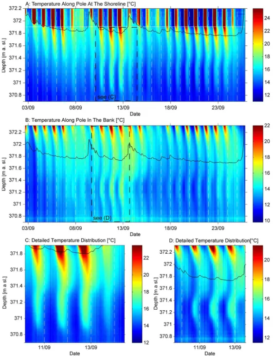
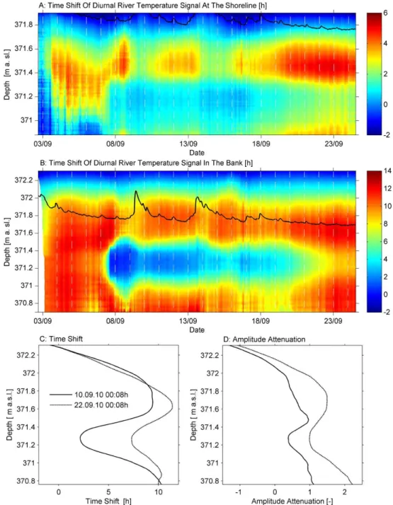
Fig. 5. Results of dynamic harmonic regression. (A)Time shift of the diurnal river signal over depth and time in the sediments at the shoreline. The black solid line indicates the water level.(B)Time shift of the diurnal river signal over depth and time in the riparian bank. The black solid line indicates the water level. (C)Temporal and vertical variability of the time shift in the bank as a function of depth during elevated water table (371.9 m a.s.l. on 10 September 2010) and low water table (371.7 m a.s.l. on 22 September 2010).(D)Temporal and vertical variability of the amplitude attenuation below groundwater table in the bank as a function of depth during elevated water table (371.9 m a.s.l. on 10 September 2010) and low water table (371.7 m a.s.l. on 22 September 2010).
the flow velocity cannot be applied here. In order to charac-terize heat transfer between the profiles at the shoreline and within the bank, we consider the time shift and amplitude attenuation as function of depth in the two profiles. Assum-ing that groundwater flow in the bank is lateral throughout the observation period, we can roughly estimate a
horizon-tal heat-transfer velocity from the difference in time shifts at identical depth and the distance between the two profiles.
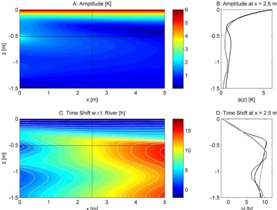
Fig. 6.Modeling results for depth varying horizontal groundwater flow velocity.(A)Simulated amplitude of the diurnal temperature signal. The horizontal black solid line indicates water the table and the vertical black dashed line shows the location of the amplitude profile.(B)
Amplitude profile at 2.5 m distance to the river (black solid line). The black dashed line represents the observed amplitude at the pole in the bank.(C)Simulated time shift of the diurnal temperature signal. The horizontal black solid line indicates water table, the vertical black dashed line shows the location of the time-shift profile, and the white lines indicate isochrones of 1 h time shift. (D)Time-shift profile at 2.5 m distance to the river (black solid line). The black dashed line represents the observed time-shift at the pole in the bank and the grey solid line shows the time-shift profile for uniform horizontal groundwater flow without velocity differences over depth.
has an average time shift of−1.75 h compared to the river temperature. In the shallow unsaturated sediments, the time shift increases almost linearly with depth, especially in the bank where an unsaturated zone continuously exists. The time shift at the shoreline reaches a first maximum of up to 5–6 h in the depth of 371.4–371.6 m a.s.l. and in the bank in 371.6–371.8 m a.s.l. a maximum of up to 11–12 h. Within the next 0.2–0.4 m below the maximum, the time shift decreases and then starts to increase again (Fig. 5c). In the bank, the upper time shift maximum is at the interface between un-saturated and un-saturated zone. By contrast, the upper time shift maximum at the shoreline lies below the water table. At the beginning of the monitoring period, a bad signal-to-noise ratio caused negative time shifts in groundwater at the shoreline. The spatiotemporal distribution of the amplitude attenuation shows nearly the same pattern (Fig. 5d). The un-saturated zone is characterized by an almost linear increase in amplitude attenuation and groundwater by high amplitude attenuation in the shallow part, then the attenuation decreases and in the deeper part increases again. In contrast to the time shift, at the unsaturated – saturated interface a stronger
in-crease of amplitude attenuation occurs, although the upper maximum of attenuation lies below the water table, too.
Besides the vertical variability, a pronounced temporal variability of heat transport exists. The special spatial pat-terns of increasing, decreasing, and again increasing time shifts with depth remain under different hydrological con-ditions. At the shoreline, the time shift distribution is patchy with shortest values when the sediments are flooded. Also in the bank the shortest time shifts occur when the water ta-ble is high, but here the locations of maximum and minimum time shifts are more stable. While the time-shift distribu-tion is constant in the unsaturated zone, groundwater exhibits the strongest temporal variations (Fig. 5c–d). In the riparian groundwater of the bank at 371.3 m a.s.l. the time shift ranges from 2 h for high and 8 h for low water table. Furthermore, the amplitude attenuation is up to 3–4 times higher at low water table conditions.
5.3 Model results
heat transport model. First, the simulations were run with a uniform horizontal groundwater velocity. Subsequently, we applied depth varying horizontal groundwater flow veloci-ties to obtain a better agreement between modeled and ob-served time shifts in riparian groundwater. The applied ver-tical distribution of horizontal velocities is sinusoidal with a minimum of 0.58×10⁻⁴m s−1in 0.7 and 1.4 m depth and fastest velocities of 1.04×10⁻⁴m s−1in the middle part of the aquifer in 0.9–1.0 m depth. These velocities are slightly slower than the roughly estimated velocities from the differ-ence in time shifts between the two profiles for 22 Septem-ber 2010 00:08 UTC +2 h, where we estimated for the pole in the bank a velocity profile of 2×10⁻⁴m s−1 in the top and deep part and fastest velocities with 4×10⁻⁴m s−1 in the middle of the groundwater profile. The presented ampli-tudes and time shifts are the simulation results for the depth varying horizontal flow velocities.
The temperature signal originating from the land surface strongly decreases in the top sediments of the unsaturated zone over the entire width of the model domain shown by the strong decrease in amplitudes (Fig. 6a). Below, horizon-tal differences occur. The amplitudes at the left side in the deeper part of the unsaturated zone become higher closer to the water table, whereas the amplitudes are decreasing with depth in the unsaturated zone on the right side. Compared to the unsaturated zone, the amplitudes in the groundwater layer are smaller with a maximum of 2.5 K in shallow groundwater close to the left heat input boundary. Amplitudes are decreas-ing with depth in the deeper part of the groundwater layer. With increasing distance from the river, the amplitude maxi-mum moves continuously deeper below the groundwater ta-ble. For illustration, Fig. 6b (black solid line) shows a verti-cal amplitude profile at 2.5 m distance to the river. This is the distance to the river of the fiber-optic high-resolution tem-perature profiler installed in the bank whose observed ampli-tudes from 22 September 2010 00:08 CEST are shown, too. In the upper part of the unsaturated zone the data agree very well, but with increasing depth small differences occur.
Figure 6c shows the time-shift distribution of the diurnal signal with respect to the river signal. In the upper part of the unsaturated zone, the time shift increases linear with depth. The time-shift distribution in the deeper part of the unsatu-rated zone and the groundwater layer is more complex, be-cause the values show a vertical variability with first decreas-ing and then again increasdecreas-ing values with depth. In flow di-rection from left to right the time shift is increasing in the groundwater layer. The zone of high vertical time-shift gra-dients in the deeper part of the unsaturated zone is moving closer to the water table with increasing distance from the river. Figure 6d shows vertical time-shift profiles to illustrate the vertical time-shift variability at 2.5 m distance to the river and to compare the simulated (black solid line) with the ob-served (black dashed line) time shift of the fiber-optic high-resolution temperature profiler installed in the bank from 22 September 2010 at 00:08 UTC +2 h. The model
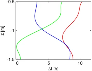
repro-Fig. 7. Simulated time-shift profiles at 2.5 m distance to the river with (red) and without (blue) heat exchange with the unsaturated zone. The green line shows the difference between both profiles and represents the time-shift error, if heat exchange is neglected.
duces the general trend of linear increase with depth in the unsaturated zone and vertical time-shift variations in ground-water, but the vertical variations of the measured groundwa-ter data are stronger. Moreover, in the simulation the first time-shift maximum lies above water table, whereas in the bank of the riverbed the time shift maximum has almost the same elevation as the water table. At the bottom of the aquifer the simulated and measured time shifts agree well with the measured data. We demonstrate the effect of depth varying horizontal groundwater flow velocities on the time-shift distribution in Fig. 6d. The shortest travel times at a depth of about 1 m reflect the zone of higher flow velocities. The grey solid line shows that uniform horizontal groundwa-ter flow velocity fails to explain the observed shortest travel times in the middle groundwater, although time shifts in shal-low and deep groundwater are well reproduced.
identical to those considering the unsaturated zone. By con-trast, thermal exchange with the unsaturated zone causes a significant additional apparent retardation of diurnal tem-perature signals in shallow groundwater. The difference in time shift is the largest with 7 h close to the water table and decreases to zero 0.75 m below water table. This im-plies that interpreting the shallow groundwater temperature signal without considering the unsaturated zone may lead to erroneous velocities by about a factor of three.
6 Discussion and conclusions
Investigating riparian groundwater flow close to losing rivers is challenging due to temporal and spatial variations. In ad-dition, field investigations are often limited by insufficient sensors spacing and their analysis by simplifying assump-tions. The focus of the present study is on using diurnal tem-perature oscillations as natural tracer for locally surveying vertical variations of lateral groundwater flow upon river wa-ter infiltration. The experimental set-up using wrapped op-tical fibers to monitor high-resolution temperature profiles is based on the study of Vogt et al. (2010b). In contrast to the latter, we use the high vertical resolution of the wrapped op-tical fibers not for verop-tical flow but for verop-tical variations of lateral flow, which may be considered typical in pre-alpine riparian zones (Huggenberger et al., 1998) and have already been hypothesized for the test site at River Thur (Doetsch et al., 2012). Such variations are caused by spatial variabil-ity of hydraulic properties in riparian sediments. In addition, we have modified and applied the numerical heat-transport model of Molina-Giraldo et al. (2011), which was originally developed to analyze the propagation of seasonal tempera-ture signals, to obtain a better understanding of the observed temperature patterns and examine the error, introduced by in-terpreting diurnal temperature oscillations using approaches neglecting heat exchange with the unsaturated zone.
The fiber-optic high-resolution monitoring of diurnal tem-perature oscillations enables detailed insights into the tempo-ral and vertical dynamics of heat transport in shallow riparian groundwater close to losing streams. Due to the high tempo-ral and vertical resolution, characteristic curve-shaped tem-perature patterns were observed in detail. Our results show that the interpretation of these profiles is difficult, because the observed distribution of temperature time shifts on the bank is influenced by several factors, namely (1) the non-uniform profile at the shore line, reflecting by itself complicated flow paths from the river to different points along the depth profile at the shore line, (2) the vertical variation of lateral ground-water flow velocities, and (3) the conductive heat exchange with the unsaturated zone. Without the high-resolution tem-perature profiles, we would have missed the curved-shaped patterns in temperature time shifts, and most likely we would have interpreted single-point time series without considering
impacts of the unsaturated zone, thus leading to erroneous lateral groundwater velocities.
Besides the vertical variations we detected that changing river stages cause temporal variability of heat transport: In our investigations, we have observed the shortest time shifts and smallest amplitude attenuation in groundwater during high river stage. In this situation, the hydraulic gradient between river and groundwater is higher, resulting in faster flow and therewith faster heat transport. Of course, the vari-ability of velocity in response to variations in river stage de-pends highly on local conditions, e.g. in the study of Cirpka et al. (2007) at a different River-Thur site, the groundwa-ter table quickly followed the river stage, so that velocity fluctuations were less pronounced.
The numerical heat transport model has qualitatively re-produced the vertical variability and curved-shape profiles of temperature amplitude and time shift within riparian ground-water. Compared to a rough estimation from the difference in observed time shifts between the profiles at the shoreline and the bank, the simulated flow velocities are about four times slower. The flow velocities, both simulated and based on field data, range between 0.6 and 4×10⁻⁴m s−1, which is typical for pre-alpine gravel aquifers. In particular, the ver-tical distribution of flow velocities with twice as high veloci-ties in the middle part compared to the shallow and deep part of the groundwater is important for future studies on biogeo-chemical processes upon river water infiltration at the test site and shows the variability of groundwater flow velocities in fluvial sediments close to losing rivers. The model, however, is simplified and was set up for a single representative flow regime and does not exactly reproduce the spatiotemporal temperature distribution.
too deep for the diurnal land-surface signal to reach ground-water, the diurnal river signal in groundwater influences the temperature distribution in the unsaturated zone by conduc-tive heat exchange. Both scenarios affect amplitude and time shift of the diurnal temperature signal in shallow riparian groundwater at a losing stream and result in a delayed diurnal river-temperature signal in shallow groundwater. Even with-out heat input at the land surface, the conductive exchange with the unsaturated zone results in a retardation of the time shift in shallow groundwater. Molina-Giraldo et al. (2011) simulated the same effect for the seasonal temperature sig-nal considering distances to the river of more than 50 m. They also had to account for heat exchange with the un-derlying aquitard. The latter was not needed in the present study, because dampening of diurnal temperature fluctua-tions is much stronger than for seasonal ones, which also explains the shorter travel distances over which the diurnal fluctuations can be observed.
The main error source for the interpretation of diurnal tem-perature oscillations in young riparian groundwater close to losing rivers lies in neglecting the thermal exchange with the unsaturated zone. The resulting retardation effect delays the travel time of the diurnal river-temperature signal by fac-tor of 3 in shallow groundwater and vanishes at the studied location about 0.75 m below the groundwater table. There-fore, the travel-time interpretation of diurnal temperature os-cillations results in underestimated exchange fluxes, if the heat exchange with the unsaturated zone in shallow riparian groundwater is not taken into account. Additional misinter-pretations of time shift by multiples of 1 d can occur, if the time until the diurnal signal is totally damped is longer than one day.
Uncertainty and error sources of our field study are related to sensor resolution as for investigations with standard tem-perature sensors, too. The time resolution of 15 min inter-vals was sufficient to monitor the diurnal temperature signal. In contrast to point measurements or sensor-chains with a sensor-depth uncertainty of up to 0.02 m, we know the ex-act depth and sensor spacing of the wrapped optical fiber. Although the depth intervals were constant over time, pos-sible changes of the land-surface elevation at the installation locations could be observed due to a sharp temperature con-trast and the high vertical resolution of the wrapped optical fiber. The high vertical resolution of the fiber-optic profil-ers and thus the detailed detection of vertical differences of heat transport are their main advantages. Interpretation of the complex temperature patterns remains vague, if a single point sensor or a chain of point sensors is applied. Conversely, compared to standard temperature sensors with a resolution of 0.02 K, DTS data are noisier. DTS noise can be attributed to the experimental set up namely the instrument’s sampling resolution/spatial resolution algorithm (Tyler et al., 2009), white and flicker noise (Su´arez et al., 2011), or altering splice connections between the wrapped fiber and the robust con-nection cable. DTS noise and precision can be improved by
increasing the measurement time interval or by manually cal-ibrating temperatures along the optical fiber as presented by Su´arez et al. (2011). If the amplitude of the diurnal signal is lower than the accuracy and noise of the measurement, which was the case below 370.7 m a.s.l. at our field site, the extrac-tion of amplitude and phase angle becomes erroneous. In general, the exact extraction of amplitudes and phase angles by means of dynamic harmonic regression is important and turned out to be a robust method even for noisy DTS-data. During sunny days, solar radiation caused warming of the fiber-optic cables exposed to air and very shallow river wa-ter as reported by Vogt et al. (2010b). However, the impact of solar radiation is similar for standard temperature sensors (Neilson et al., 2010).
Overall, we recommend high-resolution temperature pro-filers for investigations of lateral groundwater flow close to losing rivers by means of diurnal temperature oscillations, especially if vertical variations of groundwater flow can be expected. The distributed fiber-optic sensor requires only a single sensor calibration in contrast to sensor chains at mul-tiple single-point sensors. Moreover, the installation depth of single-point sensors in observation wells is difficult. If the sensor is located close to the groundwater table, the un-saturated zone affects the temperature data, and if the sen-sor is installed too deep, diurnal temperature oscillations are not detectable. Therefore, the combination of high resolu-tion field data and modeling offers a qualified approach for investigations in the complex hydraulic and thermal environ-ment of the shallow riparian groundwater close to losing river sections. Our field and modeling studies demonstrate the need for accounting thermal exchange of groundwater with the unsaturated zone when using time-shift or amplitude at-tenuation of the diurnal temperature signal for calculation of flow velocities. In contrast to well-to-well artificial tracer tests, it is impossible to understand the complex flow system completely, when a periodic signal as natural tracer is used, which is infiltrating over the entire riverbed at the test site.
Acknowledgements. This study was financed by the Competence Center Environment and Sustainability (CCES) of the ETH domain in the framework of the RECORD project (Assessment and Modeling of Coupled Ecological and Hydrological Dynamics in the Restored Corridor of a River (Restored Corridor Dynamics)). In addition, this work was supported by the Swiss National Science Foundation (SNF grant 200021-129735 “Alpine Hydrogeology”). We thank Andreas Raffainer and Peter G¨aumann of the Eawag workshop for their help in wrapping and installing the fiber-optic temperature profilers.
References
Anderson, M. P.: Heat as a ground water tracer, Ground Water, 43, 951–968, doi:10.1111/j.1745-6584.2005.00052.x, 2005. BAFU: Hydrologischer Atlas der Schweiz, Bundesamt f¨ur Umwelt,
Bern, Switzerland, 2010.
Boulton, A. J., Findlay, S., Marmonier, P., Stanley, E. H., and Valett, H. M.: The functional significance of the hyporheic zone in streams and rivers, in: Annual Review of Ecology and System-atics, edited by: Fautin, D. G., Annual Review of Ecology and Systematics: 29, Annual Reviews Inc. a, 59–81, 1998.
Cardenas, M. B.: Thermal skin effect of pipes in streambeds and its implications on groundwater flux estimation using di-urnal temperature signals, Water Resour. Res., 46, W03536, doi:10.1029/2009wr008528, 2010.
Carsel, R. and Parrish, R.: Developing joint probability distribu-tions of soil water retention characteristics, Water Resour. Res., 24, 755–769, 1988.
Cirpka, O. A., Fienen, M. N., Hofer, M., Hoehn, E., Tessarini, A., Kipfer, R., and Kitanidis, P. K.: Analyzing bank filtration by deconvoluting time series of electric conductivity, Ground Water, 45, 318–328, doi:10.1111/j.1745-6584.2006.00293.x, 2007. Constantz, J.: Heat as a tracer to determine streambed
water exchanges, Water Resour. Res., 44, W00D10, doi:10.1029/2008WR006996, 2008.
de Marsily, G.: Quantitative Hydrogeology, Academic Press, San Diego, California, 1986.
Doetsch, J., Linde, N., Pessognelli, M., Green, A. G., and G¨unther, T.: Constraining 3-D electrical resistance tomography with GPR reflection data for improved aquifer characterization, J. Appl. Geophys., 78, 68–76, doi:10.1016/j.jappgeo.2011.04.008, 2012. Domenico, P. A. and Schwartz, F. W.: Physical and chemical hy-drogeology, John Wiley & Sons Inc., New York, 528 pp., 2008. Fanelli, R. M. and Lautz, L. K.: Patterns of water, heat, and solute
flux through streambeds around small dams, Ground Water, 46, 671–687, doi:10.1111/j.1745-6584.2008.00461.x, 2008. Fleckenstein, J. H., Krause, S., Hannah, D. M., and Boano,
F.: Groundwater-surface water interactions: New meth-ods and models to improve understanding of processes and dynamics, Adv. Water Resour., 33, 1291–1295, doi:10.1016/j.advwatres.2010.09.011, 2010.
Gordon, R. P., Lautz, L. K., Briggs, M. A., and McKen-zie, J. M.: Automated calculation of vertical pore-water flux from field temperature time series using the VFLUX method and computer program, J. Hydrol., 420-421, 142-158, doi:10.1016/j.jhydrol.2011.11.053, 2012.
Goto, S., Yamano, M., and Kinoshita, M.: Thermal response of sediment with vertical fluid flow to periodic temperature vari-ation at the surface, J. Geophys. Res.-Sol. Ea., 110, B01106, doi:10.1029/2004jb003419, 2005.
Hatch, C. E., Fisher, A. T., Revenaugh, J. S., Constantz, J., and Ruehl, C.: Quantifying surface water-groundwater in-teractions using time series analysis of streambed thermal records: Method development, Water Resour. Res., 42, W10410, doi:10.1029/2005wr004787, 2006.
Hayashi, M. and Rosenberry, D. O.: Effects of ground water ex-change on the hydrology and ecology of surface water, Ground Water, 40, 309–316, 2002.
Hoehn, E. and Cirpka, O. A.: Assessing residence times of hy-porheic ground water in two alluvial flood plains of the Southern
Alps using water temperature and tracers, Hydrol. Earth Syst. Sci., 10, 553–563, doi:10.5194/hess-10-553-2006, 2006. Huggenberger, P., Hoehn, E., Beschta, R., and Woessner,
W.: Abiotic aspects of channels and floodplains in ripar-ian ecology, Freshw. Biol., 40, 407–425, doi:10.1046/j.1365-2427.1998.00371.x, 1998.
Kalbus, E., Schmidt, C., Molson, J. W., Reinstorf, F., and Schirmer, M.: Influence of aquifer and streambed heterogeneity on the dis-tribution of groundwater discharge, Hydrol. Earth Syst. Sci., 13, 69–77, doi:10.5194/hess-13-69-2009, 2009.
K¨aser, D. H., Binley, A., Heathwaite, A. L., and Krause, S.: Spatio-temporal variations of hyporheic flow in a riffle-step-pool sequence, Hydrol. Process., 23, 2138–2149, doi:10.1002/hyp.7317, 2009.
Keery, J., Binley, A., Crook, N., and Smith, J. W. N.: Temporal and spatial variability of groundwater-surface wa-ter fluxes: Development and application of an analytical method using temperature time series, J. Hydrol., 336, 1–16, doi:10.1016/j.jhydrol.2006.12.003, 2007.
Lagarias, J. C., Reeds, J. A., Wright, M. H., and Wright, P. E.: Convergence properties of the Nelder-Mead simplex method in low dimensions, Siam J. Optimiz., 9, 112–147, 1998.
Lautz, L. K.: Impacts of nonideal field conditions on vertical wa-ter velocity estimates from streambed temperature time series, Water Resour. Res., 46, W01509, doi:10.1029/2009wr007917, 2010.
Lewandowski, J., Angermann, L., Nutzmann, G., and Fleck-enstein, J. H.: A heat pulse technique for the determina-tion of small-scale flow direcdetermina-tions and flow velocities in the streambed of sand-bed streams, Hydrol. Process., 25, 3244– 3255, doi:10.1002/hyp.8062, 2011.
Molina-Giraldo, N., Bayer, P., Blum, P., and Cirpka, O. A.: Propagation of Seasonal Temperature Signals into an Aquifer upon Bank Infiltration, Ground Water, 49, 491–502, doi:10.1111/j.1745-6584.2010.00745.x, 2011.
Neilson, B. T., Hatch, C. E., Ban, H., and Tyler, S. W.: Solar radiative heating of fiber-optic cables used to moni-tor temperatures in water, Water Resour. Res., 46, W08540, doi:10.1029/2009wr008354, 2010.
Rau, G. C., Andersen, M. S., McCallum, A. M., and Acworth, R. I.: Analytical methods that use natural heat as a tracer to quantify surface water-groundwater exchange, evaluated us-ing field temperature records, Hydrogeol. J., 18, 1093–1110, doi:10.1007/s10040-010-0586-0, 2010.
Schmidt, C., Bayer-Raich, M., and Schirmer, M.: Characteriza-tion of spatial heterogeneity of groundwater-stream water in-teractions using multiple depth streambed temperature measure-ments at the reach scale, Hydrol. Earth Syst. Sci., 10, 849–859, doi:10.5194/hess-10-849-2006, 2006.
Schneider, P., Vogt, T., Schirmer, M., Doetsch, J. A., Linde, N., Pasquale, N., Perona, P., and Cirpka, O. A.: Towards Improved Instrumentation for Assessing River-1 Groundwater Interactions in a Restored River Corridor, Hydrology and Earth System Sci-ences, 15, 2531–2549, doi:10.5194/hess-15-2531-2011, 2011. Sch¨on, J. H.: Physical Properties of Rocks: Fundamentals and
Prin-ciples of Petrophysics, second ed. Pergamon, Oxford, 583 pp., 1998.
and Parlange, M. B.: Distributed fiber-optic temperature sens-ing for hydrologic systems, Water Resour. Res., 42, W12202, doi:10.1029/2006wr005326, 2006.
Shanafield, M., Hatch, C., and Pohll, G.: Uncertainty in thermal time series analysis estimates of streambed water flux, Water Re-sour. Res., 47, W03504, doi:10.1029/2010wr009574, 2011. Sheets, R. A., Darner, R. A., and Whitteberry, B. L.: Lag times of
bank filtration at a well field, Cincinnati, Ohio, USA, J. Hydrol., 266, 162–174, doi:10.1016/s0022-1694(02)00164-6, 2002. Silliman, S. E., Ramirez, J., and McCabe, R. L.: Quantifying
downflow through creek sediments using temperature time-series – One-dimensional solution incorporating measured surface-temperature, J. Hydrol., 167, 99–119, 1995.
Stallman, R. W.: Steady 1-dimensional fluid flow in a semi-infinite porous medium with sinusoidal surface temperature, J. Geophys. Res., 70, 2821–2827, 1965.
Su, G. W., Jasperse, J., Seymour, D., and Constantz, J.: Estimation of hydraulic conductivity in an alluvial system using tempera-tures, Ground Water, 42, 890–901, 2004.
Su´arez, F., Aravena, J. E., Hausner, M. B., Childress, A. E., and Tyler, S. W.: Assessment of a vertical high-resolution distributed-temperature-sensing system in a shallow thermoha-line environment, Hydrol. Earth Syst. Sci., 15, 1081–1093, doi:10.5194/hess-15-1081-2011, 2011.
Taylor, C. J., Pedregal, D. J., Young, P. C., and Tych, W.: Environmental time series analysis and forecasting with the Captain toolbox, Environ. Modell. Softw., 22, 797–814, doi:10.1016/j.envsoft.2006.03.002, 2007.
Tyler, S. W., Selker, J. S., Hausner, M. B., Hatch, C. E., Torgersen, T., Thodal, C. E., and Schladow, S. G.: Environmental tem-perature sensing using Raman spectra DTS fiber-optic methods, Water Resour. Res., 45, W00D23, doi:10.1029/2008wr007052, 2009.
van Genuchten, M. T.: A closed-form equation for predicting the hydraulic conductivity in unsaturated soils, Soil Sci. Soc. Am. J., 44, 892–898, 1980.
Vogt, T., Hoehn, E., Schneider, P., and Cirpka, O. A.: Investigation of bank filtration in gravel and sand aquifers using time-series analysis, Grundwasser, 14, 179–194, doi:10.1007/s00767-009-0108-y, 2009.
Vogt, T., Hoehn, E., Schneider, P., Freund, A., Schirmer, M., and Cirpka, O. A.: Fluctuations of electrical conductivity as a natural tracer for bank filtration in a losing stream, Adv. Water Resour., 33, 1296–1308, doi:10.1016/j.advwatres.2010.02.007, 2010a. Vogt, T., Schneider, P., Hahn-Woernle, L., and Cirpka, O. A.:
Es-timation of seepage rates in a losing stream by means of fiber-optic high-resolution vertical temperature profiling, J. Hydrol., 380, 154–164, doi:10.1016/j.jhydrol.2009.10.033, 2010b. Wroblicky, G. J., Campana, M. E., Valett, H. M., and Dahm, C. N.:
Seasonal variation in surface-subsurface water exchange and lat-eral hyporheic area of two stream-aquifer systems, Water Resour. Res., 34, 317–328, doi:10.1029/97WR03285, 1998.