Effect of marital status on duration of
treatment for mental illness
Zheng Wu
Department of Sociology, University of Victoria
[email protected]
Christoph M. Schimmele
Department of Sociology, University of Victoria
Margaret J. Penning
Department of Sociology & Centre on Aging, University of Victoria
Chi Zheng
Centre on Aging, University of Victoria
Samuel Noh
Social, Equity and Health Research Centre for Addiction and
Mental Health
Abstract
There is a well-established link between marital status and mental health, but previous research has produced mixed results about the reasons for this relationship. Some studies propose that marriage provides protection from stressors and increases personal coping abilities (the causation perspective), whereas other studies argue that marriage markets “weed out” individuals predisposed to illness (the selection perspective). This article addresses the causation-versus-selection debate by examining the effect of marital status on duration of treatment for mental illness. The empirical analysis uses longitudinal data and GEE models to estimate group-level differences in duration of treatment. The results suggest that marriage does not appear to confer a health advantage in terms of duration of treatment. However, the study demonstrates that the never-married experience longer treatment time than the married, divorced, and widowed.
Keywords: mental illness, mental health, marital status, social causation, social selection.
Résumé
Introduction
1Married people have a lower prevalence of psychological and psychiatric disorders, higher self-ratings of mental health, and more optimistic attitudes in comparison to their never-married and previously married counterparts (Bierman, Fazio, and Milkie 2006; Frech and Williams 2007; Gove, Briggs-Style, and Hughes 1990; Scott et al. 2010). Married people also have a lower rate of outpatient treat-ment for treat-mental illness, a lower rate of admission to psychiatric facilities, and a
lower suicide rate (Kessler et al. 2005; Jarman et al. 1992; Mastekaasa 1992). Of
course, sometimes marriage contributes to a higher risk of mental health prob-lems, such as within stressful, dysfunctional, or abusive relationships (Choi and Marks 2008; Horwitz, McLaughlin, and White 1998; Ratner 1998; Gove 1972). In most circumstances, however, marriage appears to decrease exposure to stressful experiences and also mitigates the health-damaging effects of exposure to stress.
The relative advantages of being married versus the de-selection of the un-healthy from marriage comprise the two principal explanations for health disparities between the married, previously married, and never-married (see Goldman 1994; Wade and Pevalin 2004; Wyke and Ford 1992). The causation-selection debate cen-ters on whether marriage decreases the probability of being ill, being ill decreases the probability of becoming or staying married, or some combination of both. The social causation perspective argues that the advantages that the married have are attributable mainly to the inherent assets and characteristics of marriage, such as
access to reliable social support and the psychological and emotional beneits of a
marital relationship. The social selection perspective argues that unhealthier people have lower chances of becoming married and higher chances of getting divorced in comparison with healthier people, and these individual-level predispositions largely account for the aforementioned differences in the prevalence of illness.
To date, the causation-selection debate has focused on an essentially theor-etical issue, i.e., whether marriage has a protective effect on health or whether marriage is selective of healthier persons. Few studies have considered whether
marital status also inluences pathways into wellness (recuperation) after disease
onset. Our objective is to explore the effect of marital status on differences in duration of treatment for mental illness. We compare 4 marital status groups: the married, never-married, separated/divorced, and widowed. This analysis provides new insight into whether marriage provides resources that improve recuperation or whether the never -married are predisposed to longer and/or more complicated
mental illnesses. If marriage confers salutogenic beneits, as the causation perspec -tive suggests, then it is reasonable to expect that, besides shielding individuals from
becoming ill, these resources also inluence the duration of illness.
Theoretical background
The causation perspective is the most salient explanation for marital status differences in mental health and there are few studies that provide empirical port for a selection effect. Horwitz and colleagues (1996) offer compelling sup-port for a causation/protective effect on the prevalence of mental illness. Their
study demonstrates that the married have lower levels of depression and alcohol-ism than the never-married, after controlling for premarital levels of depression
and alcohol use. Moreover, their indings demonstrate that becoming married has beneicial effects, which contributes to a reduction of depressive symptoms and
alcohol-related problems. The relevance of this study is that it shows that
predis-position to illness (selection) appears to be an insuficient explanation for marital
status variation in depression and alcoholism, and that marriage has a salutogenic (health-promoting) effect on pre-existing illness.
Differences in the social distribution of stress are a common explanation for marital status differences in the prevalence of mental illness, with marriage puta-tively decreasing exposure to stressful life experiences. Of course, this protective effect is moot after disease onset. However, Kessler and Essex (1982) propose an
additional mechanism through which marital status could inluence health out -comes. They argue that the married are more resilient to stress than the never-mar-ried and previously marnever-mar-ried. Marriage could be selective of people with hardier
psychological proiles or it could provide resources (e.g., social support) that im
-prove coping. Kessler and Essex conclude that the beneits associated with intim -ate relationships (conjugal unions) represent potent resources for decreasing the health-damaging effects of stress. These relationships increase coping capacities through bolstering intra-psychic resources, such as mastery and self-esteem. Since marriage confers a sense of intimacy that promotes coping, Kessler and Essex question the notion that marriage appears to contribute to health only because it
is selective of people with hardier psychological proiles, but their cross-sectional
analysis could not rule out a selection effect.
If coping can transform stress into a benign outcome, can it also transform the experience of distress? Given that marriage reduces the health-damaging ef-fects of stress through the coping process (an upstream effect) then it could also
have a similar inluence on recuperation (a downstream effect). The married could
possess two interrelated advantages in recuperation over the never-married and the previously married. First, marital status predicts resilience to stress because familial relationships are a core source of social support. There is a well-estab-lished relationship between social support and numerous health outcomes, includ-ing recovery from chronic illness (Rogers, Anthony, and Lyass 2004). Through the provision of social support, marriage fosters a rich cache of coping assets (Thoits 1986). Second, marriage is a form of social integration and provides a sense of happiness, which are important aspects of emotional and mental well-being (See-man 1996; Stack and Eshle(See-man 1998). Hence, marriage can increase coping and hardiness through boosting optimism, mastery, and self-esteem, which can help individuals recover from illness (Warner 2009).
To be sure, Ross (1995) observes that social ties are better predictors of
well-being than marital status per se. She demonstrates that the negative effect of well-being
single becomes non-signiicant after adjusting for differences in social support.
1994). Wyke and Ford (1992) demonstrate that the married have lower levels of distress than the never-married and previously married, and also have a consist-ent advantage in their number of close relatives and friends, companionship
sup-port, and quality of support. Previous research conirms that social support medi -ates the relationship between marital status and mental health outcomes, and that marriage promotes a reduction in symptoms of anxiety and depression (LaPierre 2009; Sherbourne and Hays 1990).
The following analysis considers two possible effects of marital status on duration of treatment for mental illness: a salutogenic effect and a selection effect. The concern is with the relative importance of these effects, which are not mutually exclusive (Goldman 1994; Mastekaasa 1992). If the causation perspective is ger-mane after disease onset, then the married should have a recuperation advantage over both the never -married and the previously married. This refers to the sa-lutogenic effect and suggests that resources unique to or concentrated among the presently married should promote recuperation. In contrast, a selection effect is likely present if the never-married have a recuperation disadvantage in comparison to both the married and the previously married and if the previously married do not experience a disadvantage vis-à-vis the married. Rather than representing a salutogenic advantage among the married, marital status differences in
recupera-tion could represent a disadvantage among the never-married. At least, deicits of
social support, hardiness, and other coping resources among the never-married could be more important for explaining marital status differences in recuperation than are the relative advantages of the married and previously married.
This study builds on the literature in two respects. First, the analysis esti-mates the duration of treatment for mental illness using 10 years (1990-2001) of longitudinal data, and presents an examination of marital status differences in long-term disease outcomes, which is unique from examining a reduction in symp-toms. A long-term follow-up is key for understanding marital status differences in duration of treatment because mental illnesses can involve a long route toward a recuperated state. In addition, our measurement of duration of treatment for mental illness is precise as it is based on the number of days of treatment. Second, the analysis uses a comprehensive measure of mental illness, including alcohol/ substance abuse, psychoses, mood disorders, dementia, and other conditions, al-lowing us to control for type of illness and comorbidity. These measures are based on clinician-based diagnoses, which are preferable to scale-based measures con-structed from patient interviews (self-reports).
Data and method
Study sample
The BC Linked Health Database (BCLHD), which is housed at the University of British Columbia, Centre for Health Services and Policy Research, is the data source for this study. The BCLHD consists of multiple, linkable datasets,
on a complete population, i.e., all public health care users in British Columbia, Canada. In this study, the target population includes all BC residents who received in- or outpatient treatment for a mental illness (termed a care episode in BCLHD records) in 1990.2 The current study was based on a simple random sample of 10
per cent of the target population over the period of 1990-2001.3 The study sample
further excludes individuals less than 18 years old and cases missing key variables
(e.g., duration of treatment and marital status). The inal study sample includes 7,588 individuals and a total of 10,137 care episodes.4 All care episodes are
com-plete for respondents with admission dates in 1990 and discharge dates before or during 2001. The data for ongoing (censored) care episodes are unavailable.
Dependent Variable
Our dependent variable is duration of treatment for mental illness, under the care of a health care professional, which represents a route toward a recuperated state, because in most (albeit not all) cases formal treatment continues until a substantial resolution of or effective management of symptoms is achieved.5 The dependent variable is time-invariant at the episode level, but time-variant at the individual-level in cases where a respondent received treatment for a relapse or the
onset of a new illness after recuperation from a previous illness. We deine treat -ment for -mental illness as all MSP-billable hospitalizations and/or outpatient treat-ments from a health care professional, such as a general physician, psychiatrist, registered psychologist, or counselor. Our focus is on marital status differences in the duration of treatment. To measure this, we subtracted the date of treatment
termination (when patient’s case ile was closed) from the date of initial diagnosis,
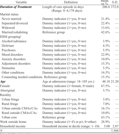
which yields a measure of days of treatment. Using data on treatments starting in 1990, Table 1 shows that the mean value for the outcome variable is 206 days of treatment with a standard deviation of 372 days.
2. Our target population includes individuals receiving treatment for a mental illness covered by public health insurance. Under the Canada Health Act (1984), all provincial governments are obliged to provide legal Canadian residents with equitable access to medically necessary services, including regular check-ups, physician consultations, outpatient treatments, specialist care, surgical procedures, and hospitalizations (Health Canada 2001). In British Columbia, this is provided through the Medical Services Plan (MSP), which is a single-payer health insurance program.
3. Only 10 per cent of the data were available for the analysis. However, the study sample is representative of the target population.
4. In 2001, 12.4 per cent of the BC adults (397,000 persons) experienced a mental illness, according to the 2002 Canadian Community Health Survey (CCHS) on Mental Health and Well-Being (see Lesage et al. 2006). The 2001 provincial utilization rate of public health care services for mental illness was 6.6 per cent, totaling 210,000 adults.
5. Given that mental illnesses can be chronic disorders (long-lasting or recurrent),
the termination of treatment often does not always represent recovery in the conventional sense (absence of symptoms), but represents recuperation in the sense that there is a reasonable level of control or management of symptoms. This is an
important step in the recovery process. See Anthony (1993) for a deinition and
Independent Variables
We measured marital status using a four-level categorical variable, including never-married, separated/divorced, widowed, and married/cohabiting (reference group).6 The information on marital status was collected at the initial contact with
a health care professional. Unfortunately, data on marital history and marital tran-sitions over the period of observation are unavailable. Hence, it is possible that some married patients may have experienced a marital disruption during the treat-ment and some unmarried patients may have become married. This could reduce
6. Data limitations prevented us from separating cohabitation from marriage. In Canada, the married and cohabitors are similar in their (a) mental health status and (b) level of social resources (Schimmele and Wu 2011; Wu, Penning, Pollard, and Hart 2003). This implies that it is not inappropriate to combine the married and cohabiting for our purposes, especially in comparing them to the never-married.
Table 1. Deinitions and descriptive statistics of the variables used in the analysis:
British Columbian (Canada) adults (aged 18+), 1990.
Variable Deinition Mean or % S.D.
Duration of Treatment Length of care episode in days
(Range: 0–4,178 days)
206.0 372.0
Marital status
Never married Dummy indicator (1=yes, 0=no) 21.4% —
Separated/divorced Dummy indicator (1=yes, 0=no) 22.4% —
Widowed Dummy indicator (1=yes, 0=no) 13.6% —
Married/cohabiting Reference group 42.6% —
DSM groupinga
Alcohol/substance Dummy indicator (1=yes, 0=no) 3.9% —
Delirium Dummy indicator (1=yes, 0=no) 4.3% —
Psychoses Dummy indicator (1=yes, 0=no) 5.5% —
Mood disorders Dummy indicator (1=yes, 0=no) 22.9% —
Anxiety disorders Dummy indicator (1=yes, 0=no) 10.8% —
Adjustment disorders Dummy indicator (1=yes, 0=no) 15.3% —
Dementia Dummy indicator (1=yes, 0=no) 5.5% —
Other conditions Dummy indicator (1=yes, 0=no) 16.5% —
Counseling needed conditions Reference group 15.3% —
Age Age at admission (range: 18–105 yrs.) 48.10 21.20
Female Dummy indicator (1=female, 0=male) 67.5% —
Aboriginal Dummy indicator (1=yes, 0=no) 3.7% —
Rurality
Urban fringe Dummy indicator (1=yes, 0=no) 3.8% —
Rural fringe Dummy indicator (1=yes, 0=no) 7.0% —
Urban outside CMAs/CAs Dummy indicator (1=yes, 0=no) 16.1% —
Rural outside CMAs/CAs Dummy indicator (1=yes, 0=no) 10.0% —
Urban core Reference group 63.1% —
Work outside home Dummy indicator (1=f/t or p/t, 0=other) 28.9% —
Household income Household income in decile (range: 1–10) 5.00 2.87
N 7,588
115
the differences in length of treatment between married, never-married, and separ-ated/divorced patients. Table 1 presents the descriptive statistics for marital status and all selected variables using individual-level data in 1990. Table 1 indicates that 21 per cent of the selected mental health patients were never-married. The
com-parable igures for separated/divorced, widowed, and married/cohabiting were
22, 14, and 43 per cent, respectively.
Mental illness was deined based on Diagnostic Statistical Manual of Mental
Disorders (DSM-IV) codes that were grouped (by a professional psychiatrist) into 9 taxonomical variables: (1) alcohol/substance abuse, (2) delirium (confusion from medical causes), (3) psychoses (schizophrenias), (4) mood disorders (depression,
bipolar disorder), (5) anxiety (panic disorder, social phobia, personality disorder,
and other neuroses such as factitious disorders, dissociations), (6) adjustment dis-order (e.g., psychiatric symptoms resulting from or directly relating to a stressor), (7) dementia (e.g., Alzheimer’s), (8) counseling needed conditions (conditions such
as bereavement, relationship dificulties, school-related problems), and (9) other
disorders (e.g., sexual identity disorders, physiological sexual disorders, sleep dis-orders, pain disdis-orders, side effects from medications). In general, the most salient
disorders were mood disorders (23 per cent), adjustment disorder (15 per cent), counseling needed conditions (15 per cent), and anxiety disorders (11 per cent).
The analysis controls for differences in type of mental illness (including comorbid conditions) under treatment.
The study includes several demographic variables available in the BCLHD. The study introduced a control variable for age, measured in years, because age
can inluence the prevalence of mental illness (Health Canada 2002). The study
includes a dummy indicator for gender, because there are gender differences in the remission of mental illness (Schimmele, Wu, and Penning 2009). The study
includes an Aboriginal status variable as this inluences mental illness (Kirmayer,
Brass, and Tait 2000). Using merged census data, the study includes a measure of rural-urban proximity developed by Statistics Canada (du Plessis, Beshiri, and
Bollman 2001), which relects geographic accessibility to specialist health services.
Finally, the study includes two measures of socioeconomic status (employment
status and household income) because ability to pay could inluence access to
pharmacological treatments. Employment status is measured using a dummy indi-cator for working outside the home. Although, income data are unavailable from
patient iles, the BCLHD provides a proxy measure of household income, created from geo-code iles of the Census. Household income is measured using income
deciles, with 1 representing the lowest and 10 the highest income bracket.
Statistical Models
pa-tients of other marital statuses. The GEE model allows for the number and spacing of the repeated measurements to vary between individuals. Like GLMs, the GEE model assumes that the response distribution belongs to the exponential family of distributions, which includes the Normal, binomial, Poisson, and other commonly used probability distributions. The parameters are estimated on the basis of quasi-likelihood theory, using an iteration algorithm to solve the score function.
The GEE model assumes that observations from each individual are correl-ated, though observations between individuals are assumed to be independent. Thus, it requires a working model (correlation matrix) for the association among observations (Diggle et al. 2002). We assume that the correlation is constant (ex-changeable) between any two observation times and use an exchangeable
cor-relation model. The GEE estimates of regression coeficients and their variances
are always consistent even when the structure of correlation matrix is incorrectly
speciied (Stokes, Davis, and Koch 2000). The loss of eficiency due to a mis-speciied correlation matrix is generally inconsequential when the sample size is
large. In this study, the GEE models were estimated using the GENMOD proced-ure in SAS 9.2 (SAS Institute 2009).
Since we decided to use the GEE model for our data analysis, we needed to make an assumption about the response (error) distribution. The dependent vari-able in this study is the number of days under treatment, measured (recorded) as a discrete count variable and contains only non-negative integers, 0, 1, 2, …, 4,178 (see Table 1). Given these characteristics, some would consider using the Poisson
model because the response distribution its into the range of the Poisson distri -bution (e.g., Long 1997; Powers and Xie 2000).7 However, it is well-known that the
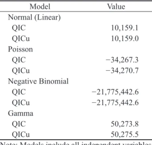
underlying assumption of the Poisson model is that the predicted mean equals the observed variance of the distribution. This assumption is not always realistic because count data are sometimes overly dispersed (when the observed variance exceeds the predicted mean). Although there are several strategies to model dis-persed data (see McCullagh and Nelder 1989), a common approach is to use the negative binomial distribution, which is also appropriate for count data and does not require the assumption that the predicted mean is equal to the observed vari-ance of the distribution. To evaluate this assumption and compare models with competing distribution assumptions, we estimated GEE models based on four distributions: the Normal, Poisson, negative binomial, and Gamma. The linear model uses the identity link function, while the rest employ the log link function. We use the full set of the explanatory variables shown in Table 1.
Table 2 presents selected measures of goodness-of-it for these four models.
Because the GEE method is based on the quasi-likelihood theory, conventional
likelihood-based measures of goodness-of-it, such as likelihood ratio test, Pear -son’s Chi-square statistic, and deviance which are widely used for model selection in GLMs, are not directly applicable to the GEE method. To address this issue, Pan (2001) proposed the QIC (quasi-likelihood under the independence model
criterion) statistic as a measure of model selection. QIC is a modiication of the 7. At suggestion of one anonymous reviewer, we transformed the dependent variable
by taking the natural logarithm. With the logged dependent variable, we re-estimated the full model in Table 4. The results are very similar to those shown in Table 4,
although the overall it statistics show marginal improvement over those of the OLS
Akaike Information Criterion (AIC), which is a common (information) measure
for comparing model its in GLMs. A related statistic, QICu, is deined as Q + 2p, which adds a penalty (2p, where p is the number of parameters in the model) to
the quasi-likelihood. When comparing model its, a smaller statistic indicates a bet
-ter it. It is obvious that selected goodness-of-it measures vary widely across the
models. The negative binomial model has the smallest QIC and QICu, indicating
a better it than the other models. For this reason, we report the results from the
negative binomial models.
There is one other methodological issue that may threaten the validity of our GEE estimates. As noted, our data are clearly overly dispersed and may have poten-tial extreme data (outliers) that can bias our GEE estimates (Diggle et al. 2002). We
examined both Pearson’s and deviance residual plots and conirmed the presence
of a small number of residuals that are relatively large. As a precautionary measure, we re-estimated models in Table 4 with an alternative estimation method, known as “Quadratic Inference Function” (QIF). As an extension of GEE, the QIF was designed to provide robust regression estimates in the presence of outliers in longi-tudinal data (Qu and Li 2006). We compared the two sets of regression estimates and observed no substantive differences between them. We decided to report the GEE estimates as the GEE is a much more mature and widely used analytical pro-cedure than the QIF. (The QIF estimates are available from the authors).8
Results
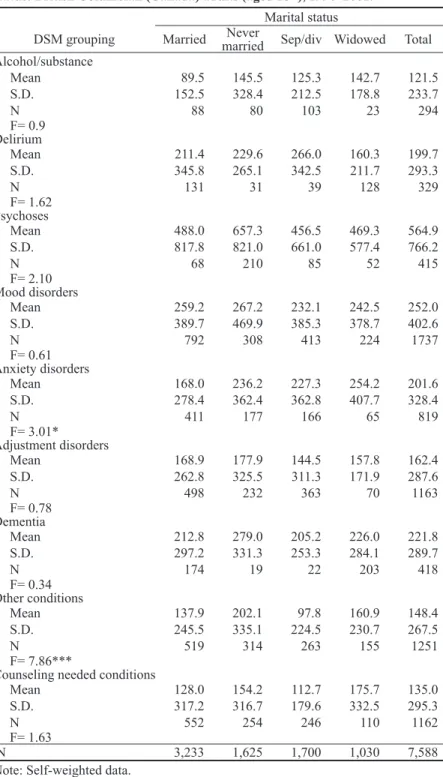
Table 3 presents bivariate statistics for average duration of treatment by ill-ness type (DSM grouping) and marital status. The marginal totals indicate an over-all average of 122 days of treatment for alcohol/substance addiction, 200 days for
8. The QIF models were estimated using a SAS macro available online: http://www-personal.umich.edu/~pxsong/qif_package.html.
Table 2 Goodness-of-it statistics (QIC and QICu) for GEE models based on the
normal, Poisson, negative binomial, and gamma distributions.
Model Value
Normal (Linear)
QIC 10,159.1
QICu 10,159.0
Poisson
QIC −34,267.3
QICu −34,270.7
Negative Binomial
QIC −21,775,442.6
QICu −21,775,442.6
Gamma
QIC 50,273.8
QICu 50,275.5
delirium, 565 days for psychoses, 252 days for mood disorders, 202 days for anx -iety disorders, 162 days for adjustment disorders, 222 days for dementia, 148 days
for “other conditions” (see deinition above), and 135 days for counseling needed
conditions. The standard deviations are large in all instances, illustrating that there is large variation in treatment times within each DSM grouping. As the F tests demonstrate, except for anxiety disorders and “other conditions,” there appear to be no marital status differences in average duration of treatment.
Table 3 provides two important, albeit preliminary, insights into the causation-selection debate. First, the married do not appear to have a consistent advantage in duration of treatment. The married have the shortest duration of treatment for alcohol or substance abuse and anxiety-related disorders and the second shortest for delirium, dementia, “other conditions,” and counseling needed conditions. But they require more treatment for psychoses, mood disorders, and adjustment dis-orders, in comparison to the previously married. The separated/divorced have the shortest duration of treatment for 6 of 9 DSM groupings, including psychoses, mood disorders, adjustment disorder, dementia, other conditions, and counseling needed conditions.
Second, the never-married have a consistent disadvantage in duration of treatment. For 6 of 9 selected DSM groupings, they require more treatment on average than the married or previously married. For the other 3 groupings, they ex-perience the second longest treatment times. For no DSM grouping do they pos-sess a treatment advantage over the married, although in some cases (e.g., mood disorders, adjustment disorders) the difference appears to be modest. There is a large difference between the never-married and the married and previously
mar-ried in duration of treatment for psychoses. The never-marmar-ried require 657 days of treatment for psychoses, in contrast to 456 days for the separated/divorced,
469 days for the widowed, and 488 days for the married. The never-married also need considerably more treatment for dementia and other disorders.
Table 4 presents the GEE analysis for the effects of marital status on
dur-ation of treatment for mental illness. The goodness-of-it statistics (see bottom of table) indicate signiicant improvements in the model it of the nested models.
Model 1 (baseline model) considers marital status differences in duration of treatment controlling for the condition (including comorbidity) under treatment. As Table 3 indicates, there are potential differences in average length of treatment across different conditions (DSM groupings). In accordance, the type of mental illness and psychiatric comorbidity may contribute to variation in duration of ment. Model 1 examines whether marital status differences in duration of treat-ment are spurious of type of illness and comorbidity. The model demonstrates that marital status has an independent effect on duration of treatment, net of type
of illness and comorbidity. In this model, duration of treatment is signiicantly (p < .001) longer for the never-married in comparison to the married. This differ -ence does not appear to represent a health advantage (salutogenic effect) inherent to marriage, because the differences in duration of treatment between the married
and the previously married are non-signiicant. The model also demonstrates that
the never-married require longer treatment than the previously married.
Table 3. Average duration of treatment (days) by DSM grouping and marital status: British Columbian (Canada) adults (aged 18+), 1990–2001.
Marital status
DSM grouping Married marriedNever Sep/div Widowed Total
Alcohol/substance
Mean 89.5 145.5 125.3 142.7 121.5
S.D. 152.5 328.4 212.5 178.8 233.7
N 88 80 103 23 294
F= 0.9 Delirium
Mean 211.4 229.6 266.0 160.3 199.7
S.D. 345.8 265.1 342.5 211.7 293.3
N 131 31 39 128 329
F= 1.62 Psychoses
Mean 488.0 657.3 456.5 469.3 564.9
S.D. 817.8 821.0 661.0 577.4 766.2
N 68 210 85 52 415
F= 2.10 Mood disorders
Mean 259.2 267.2 232.1 242.5 252.0
S.D. 389.7 469.9 385.3 378.7 402.6
N 792 308 413 224 1737
F= 0.61 Anxiety disorders
Mean 168.0 236.2 227.3 254.2 201.6
S.D. 278.4 362.4 362.8 407.7 328.4
N 411 177 166 65 819
F= 3.01* Adjustment disorders
Mean 168.9 177.9 144.5 157.8 162.4
S.D. 262.8 325.5 311.3 171.9 287.6
N 498 232 363 70 1163
F= 0.78 Dementia
Mean 212.8 279.0 205.2 226.0 221.8
S.D. 297.2 331.3 253.3 284.1 289.7
N 174 19 22 203 418
F= 0.34 Other conditions
Mean 137.9 202.1 97.8 160.9 148.4
S.D. 245.5 335.1 224.5 230.7 267.5
N 519 314 263 155 1251
F= 7.86***
Counseling needed conditions
Mean 128.0 154.2 112.7 175.7 135.0
S.D. 317.2 316.7 179.6 332.5 295.3
N 552 254 246 110 1162
F= 1.63
N 3,233 1,625 1,700 1,030 7,588
relect demographic differences. The model shows that marital status has an in -dependent effect on duration of treatment, net of these demographic variables. In the model, the disadvantage in recuperation among the never-married persists and the magnitude of this negative effect increases.
Model 3 adds socioeconomic control variables to the baseline variables. Al-though our target population are people receiving publically-funded medical
treat-ment, it is possible that SES inluences duration of treatment through differences
in access to prescription medications or via indirect mechanisms. For example, household poverty could represent an additional life strain that impedes the cop-ing process. Model 3 demonstrates that marital status differences in duration of treatment are independent of differences in SES. Introducing controls for SES does not greatly change the pattern observed in Model 1.
Model 4 combines all selected control variables and provides the most
pref-erable model it. The model demonstrates that the never-married have a general
disadvantage in duration of treatment in comparison to all other marital status
groups, which supports the selection effect. There are no signiicant differences
between the married and the previously married. Though the differences are
non-signiicant, the direction of the signs of the coeficients indicates that the previ
-ously married have a small advantage over the married. At least, these indings rule
out the salutogenic effect.
Table 4 also presents the effects of the selected control variables on duration of treatment. In comparison with counseling needed conditions, all but two DSM
groupings show signiicant effects (negative) on duration of treatment. The two
exceptions are alcohol/substance abuse and other conditions. This is unsurprising as delirium, psychoses, mood disorders, anxiety disorder, adjustment disorder, and
dementia tend to be comparatively more serious and dificult conditions to treat. The effect of age on length of treatment is signiicant and non-linear. Age has
an inverted U-shaped effect, which indicates an association between middle-age and longer treatment time. Females experience a longer duration of treatment than males. Aboriginals have shorter treatment times than non-aboriginal patients.
Though we observe some signiicant differences, there is no consistent pattern
for the effect of rurality on duration of treatment. Higher household income and employment decrease duration of treatment.
Conclusions
This study examined whether marriage promotes recuperation from mental illness (salutogenic effect) or whether the never-married are prone to longer
per-iods of illness (selection effect). The study conirms that the never-married experi -ence a longer average duration of treatment for mental illness than the married
and previously married. In addition, our indings demonstrate that the previously
Data limitations prevented a consideration of the effect of marital transi-tions (e.g., divorce) on length of treatment. A difference between the married and the separated/divorced could emerge if all separated/divorced individuals were counted accurately rather than some counted as presently married. We cannot
make irm conclusions without controls for marital transitions, but if the respond
-Table 4. Generalized estimating equations of duration of treatment on marital status and selected explanatory variables: British Columbian (Canada) adults (aged 18+), 1990–2001.
Variable Model 1 Model 2 Model 3 Model 4
Marital status
Never married 0.204*** 0.422*** 0.174*** 0.382***
Separated/divorced -0.035 -0.037 -0.066 -0.072
Widowed 0.077 -0.046 0.015 -0.057
Married/cohabitinga
Contrast (χ2with df=1)
Never married vs sep/div 19.00*** 52.51*** 19.80*** 53.48***
Never married vs widowed 4.70* 38.76*** 7.40** 35.08***
Sep/div vs widowed 3.61 0.02 1.99 0.05
DSM grouping
Alcohol/substance -0.047 -0.024 -0.075 -0.045
Delirium 0.368*** 0.296** 0.306** 0.274**
Psychoses 1.216*** 1.188*** 1.162*** 1.144***
Mood disorders 0.663*** 0.630*** 0.644*** 0.618***
Anxiety disorders 0.401*** 0.403*** 0.398*** 0.399***
Adjustment disorders 0.208** 0.229*** 0.225*** 0.236***
Dementia 0.453*** 0.362*** 0.399*** 0.360***
Other conditions 0.058 0.079 0.047 0.078
Counseling needed conditionsa
Age — 0.037*** — 0.038***
Age square — -0.0003*** — -0.0003***
Female (1=yes) — 0.128*** — 0.124**
Aboriginal (1=yes) — -0.237** — -0.223*
Rurality
Urban fringe — 0.042 — 0.070
Rural fringe — -0.064 — -0.016
Urban areas outside CMAs/CAs — 0.053 — 0.089
Rural areas outside CMAs/CAs — -0.129* — -0.114*
Urban corea
Work outside home (1=yes) — — -0.207*** -0.168***
Household income — — -0.026*** -0.025***
Intercept 4.837*** 3.710*** 5.052*** 3.911***
QIC -20787582.8 -20875485.4 -21737267.8 -21775442.6
QICu -20787582.4 -20875484.9 -21737267.7 -21775442.6
∆ QIC — 87903 949685 987860
aReference category.
bQIC difference between model 1 and model 2, model 3, and model 4, respectively.
ents who experienced a separation/divorce were removed, then the difference be-tween the married and the never-married would increase. What does this suggest about our conclusions? First, we have to assume that our comparison between the married and the never-married is somewhat conservative, because the married group could include some unmarried people. Second, the comparison between the married and the previously married could also be conservative. The lingering ques-tion is whether a difference between the married and the previously married would emerge if union transitions were controlled. Even so, it is highly unlikely that our conclusion about the salutogenic effect is incorrect because the direction of the
signs on the coeficients suggests that duration of treatment is shorter among the previously married than for the married.
Another potential data limitation is sample selection bias. Given that our study sample consists of individuals under treatment for a mental illness, there could be a sample selection bias if there are large marital status differences in treatment-seeking behaviors. For example, it is plausible that spousal advice com-pels the married to seek out treatment in higher proportions than the unmarried. In accordance, we could not observe “true” marital status differences in length of treatment of mental illness if a disproportionate number of the never-married do not get treatment. That said, previous studies demonstrate that there is a
non-signiicant difference between the married and the never-married in the utilization
of mental health services (e.g., Kimerling et al. 1999; MacKenzie, Gekoski, and Knox 2006; Mojtabai and Olfson 2006).
Though there is some evidence for a selection effect (see Mastekaasa 1992), marital status differences in the prevalence of mental illness are not entirely attrib-utable to the selection effect. Prior research indicates that people’s mental health tends to improve upon marriage, which suggests that marriage confer salutogenic
beneits (Frech and Williams 1982; Horwitz et al. 1996). This study addressed whether the salutogenic beneits that shield people from getting ill also speed the recuperation process after the onset of illness. Our indings demonstrate that these beneits appear to have limited effects on the duration of treatment of men
-tal illness. Our indings also indicate that there is the potential that being never-married impedes the recuperation process. Of course, our results are dificult to
decipher because we could not pinpoint whether marriage improves recuperation, never-married status complicates recuperation, or if a dual effect is occurring. We consider the latter option at face-value because we cannot believe that social sup-port differences between the married and the never-married are irrelevant in ex-plaining these health disparities, but neither can we ignore the implications of the
non-signiicant difference in recuperation from mental illness between the married
and the previously married. Whatever the case, our results raise questions about
the beneits of marriage for recuperation from mental illness and suggest that
something about the never-married increases their time under treatment.
References
Anthony, W.A. 1993. Recovery from mental illness: The guiding vision of the mental health service system in the 1990s. Psychological Rehabilitation Journal 16:11–23. Bierman, A., E.M. Fazio, and M.A. Milkie. 2006. A multifaceted approach to the mental
Chamberlayne, R., B. Green, M.L. Barer, C. Hertzman, W.J. Lawrence, and S.B. Sheps. 1998. Creating a population-based linked health database: A new resource for health services research. Canadian Journal of Public Health 89:270–3.
Choi, H. and N.F. Marks. 2008. Marital conlict, depressive symptoms, and functional
impairment. Journal of Marriage and Family 70:377–90.
Diggle, P.J., P. Heagerty, K.-Y. Liang, and S.L. Zeger. 2002. The Analysis of Longitudinal Data. 2nd edn. Oxford: Oxford University Press.
du Plessis, V., R. Beshiri, and R.D. Bollman. 2001. Deinitions of ‘rural’. Rural and Small Town Canada Analysis Bulletin 3:1–17.
Frech, A. and K. Williams. 2007. Depression and the psychological beneits of entering
marriage. Journal of Health and Social Behavior 48:149–63.
Goldman, N. 1994. Social factors and health: The causation-selection issue revisited. Proceedings of the National Academy of Sciences 91:1251–5.
Gove, W.R. 1972. The relationship between sex roles, marital status, and mental illness. Social Forces 51:34–44.
Gove, W.R., C. Briggs-Style, and M. Hughes. 1990. The effect of marriage on the well-being of adults. Journal of Family Issues 11:4–35.
Health Canada. 2001. Canada Health Act. Ottawa, ON: Minister of Public Works and Government Services.
———. 2002. A Report on Mental Illnesses in Canada. Ottawa: Health Canada. Horwitz, A.V., H. Raskin-White, and S. Howell-White. 1996. Becoming married and
mental health: A longitudinal study of a cohort of young adults. Journal of Marriage and the Family 58:895–907.
Horwitz, A.V., J. McLaughlin, and H. Raskin-White. 1998. How the negative and positive aspects of partner relationships affect the mental health of young married people. Journal of Health and Social Behavior 39:124–36.
Jarman, B., S. Jirsch, P. White, and R. Driscoll. 1992. Predicting psychiatric admission rates. British Medical Journal 304:1146–51.
Kessler, R.C. and M. Essex. 1982. Marital status and depression: The importance of coping resources. Social Forces 61:484–507.
Kessler, R.C., O. Demler, R.G. Frank, M. Olfson, H.A. Pincus, E.E. Walters, P. Wang, K.B.
Wells, and A.M. Zaslavsky. 2005. Prevalence and treatment of mental disorders, 1990
to 2003. New England Journal of Medicine 352:2515–23.
Kirmayer, L.J., G.M. Brass, and C.L. Tait. 2000. The mental health of aboriginal peoples: Transformations of identity and community. Canadian Journal of Psychiatry 45:607–16. Kimerling, R., P.C. Ouimette, R.C. Cronkite, and R.H. Moos. 1999. Depression and
outpatient medical utilization: A naturalistic 10-year follow-up. Annals of Behavioral Medicine 21:317–21.
LaPierre, T.A. 2009. Marital status and depressive symptoms over time: Age and gender variations. Family Relations 58:404–16.
Liang, K.-Y. and S.L. Zeger. 1986. Longitudinal data analysis using generalized linear models. Biometrika 73:13–22.
Lesage, A., H.-M. Vasiliadis, M.-A. Gagné, S. Dudgeon, N. Kasman, and C. Hay. 2006. Prevalence of Mental Illness and Related Service Utilization in Canada: An Analysis of the Canadian Community Health Survey. Mississauga, ON: Canadian Collaborative Health Initiative.
Long, S.J. 1997. Regression Models for Categorical and Limited Dependent Variables. Thousand Oaks, CA: Sage.
MacKenzie, C.S., W.L. Gekoski, and V.J. Knox. 2006. Age, gender, and the underutilization
Mastekaasa, A. 1992. Marriage and psychological well-being: Some evidence on selection into marriage. Journal of Marriage and Family 53:901–11.
McCullagh, P. and J.A. Nelder. 1989. Generalized Linear Models. 2nd edn. London: Chapman and Hall.
Mojtabai, R. and M. Olfson. 2006. Treatment seeking for depression in Canada and the United States. Psychiatric Services 57:631–9.
Pan, W. 2001. Akaike’s information criterion in generalized estimating equations. Biometrics
57:120–5.
Powers, D.A. and Yu Xie. 2000. Statistical Methods for Categorical Data Analysis. San Diego, CA: Academic Press.
Qu, A. and R. Li. 2006. Quadratic inference functions for varying-coeficient models with
longitudinal data. Biometrics 62:379–91.
Ratner, P.A. 1998. Modeling acts of aggression and dominance as wife abuse and exploring their adverse health effects. Journal of Marriage and the Family 60:453–65. Rogers, E.S., W. Anthony, andA. Lyass. 2004. The nature and dimensions of social
support among individuals with severe mental illness. Community Mental Health Journal
40:437–50.
Ross, C.E. 1995. Reconceptualizing marriage as a continuum of social attachment. Journal of Marriage and the Family 57:129–40.
SAS Institute. 2009. SAS/STAT 9.2 User’s Guide. 2nd edn. Cary, NC: SAS Institute Inc. Schimmele, C.M. and Z. Wu. 2011. Cohabitation and social engagement. Canadian Studies
in Population 38:23–36.
Schimmele, C.M., Z. Wu, and M.J. Penning. 2009. Gender and remission of mental illness. Canadian Journal of Public Health 100:353–6.
Scott, K.M., J.E. Wells, M. Angermeyer, et al. 2010. Gender and the relationship between
marital status and irst onset of mood, anxiety, and substance abuse disorders.
Psychological Medicine 40:1495–1505.
Seeman, T.E. 1996. Social ties and health: The beneits of social integration. Annals of Epidemiology 6:442–51.
Sherbourne, C.D. and R.D. Hays. 1990. Marital status, social support, and health transitions in chronic disease patients. Journal of Health and Social Behavior 31:328–43. Stack, S. and J.R. Eshleman. 1998. Marital status and happiness: A 17-nation study. Journal
of Marriage and Family 60:527–36.
Stokes, M.E., C.S. Davis, and G.G. Koch. 2000. Categorical Data Analysis Using the SAS System. 2nd edn. Cary, NC: SAS Institute.
Thoits, P.A. 1986. Social support as coping assistance. Journal of Consulting and Clinical Psychology 54:416–23.
Turner, R.J. and F. Marino. 1994. Social support and social structure: A descriptive epidemiology. Journal of Health and Social Behavior 35:193–212.
Wade, T.J. and D.J. Pevalin. 2004. Marital transitions and mental health. Journal of Health and Social Behavior 45:155–70.
Warner, R. 2009. Recovery from schizophrenia and the recovery model. Current Opinion in Psychiatry 22:374–80.
Wu, Z., M.J. Penning, M.S. Pollard, and R. Hart. 2003. ‘In sickness and in health’: Does cohabitation count? Journal of Family Issues 24:811–38.