Predicting GDP growth in the Euro Area

(1)

A Work Project, presented as part of the requirements for the Award of a Master Degree in Finance from the NOVA – School of Business and Economics

PREDICTING GDP GROWTH IN THE EURO AREA

CLÁUDIA CRISTINA MARINHO CAMPOS 418

A project carried out on the Corporate Finance Major, under the supervision of: Paulo M. M. Rodrigues

(2)

2

Predicting GDP growth in the Euro Area

Abstract

Predicting GDP growth is a concern of several economic agents. The right way to model such variable is far from consensual. This paper’s goal is to compare different models for GDP growth forecasting in the euro area. For comparative purposes, an autoregressive model (which is used as benchmark) and two Autoregressive Distributed Models (ADL), which contain financial and non-financial variables, chosen based on the literature, are used. The main conclusion is that the ADL(2,1,1) considered has superior forecast performance in- and out-of-sample, although in this last case depending on the evaluation metric.

(3)

3

1 Introduction

A vast literature in finance and macroeconomics is dedicated to the forecasting ability of financial variables for real economic activity. Since GDP growth is one of the most important macroeconomic indicators and, consequently, the main subject of interest for both society and policymakers, forecasting GDP is probably one of the most discussed topics in the literature. However, empirical evidence is mixed and results are not robust with respect to model specification, sample choice and forecast horizon, as well as, to the variables that should be used.

GDP measures economic output, representing business activity and supporting the

country’s level of productivity. On the one hand, economists rely on GDP data to

determine whether we are in expansion or contraction, while on the other hand, monetary policymakers use GDP when measuring the state of the economy and inflation. This economic indicator gains therefore an enormous relevance for several

agents’interest in the economy’s wealth and future direction (expansion or recession).

Finding a way to model such a variable is far from consensual and it has been intensively studied in the past. Hence, it is of interest to find a good model to predict GDP.

Empirical studies often choose financial variables that are considered as leading indicators of economic activity, such as stock returns, interest rates, interest rates spreads, monetary aggregates, and others. Banerjee et al. (2003) using an extensive list

of leading indicators for output growth found that measures of short and long-term interest rates, as well as interest rate spreads are the best performing single indicators for GDP growth. Furthermore, Moneta (2005) found that the yield spread is a powerful variable for predicting recessions in the euro area, a result that was also confirmed by

e.g Duarte et al. (2005), who used aggregated data for the euro area and observed the

(4)

4

that consider that the separate use of the long-term and the short-term interest rate is more powerful than the yield curve. Moreover, there is empirical evidence that the forecasting ability of the term spread has decreased over the past decade. For instance, Haubrich and Dombrosky (1996) and Dotsey (1998) confirmed, using US data and linear models, that from 1985 there is a sharp decrease in the predictability power of the term spread. In addition to these studies, we can further identify other works suggesting that the term structure and monetary aggregates are associated with future economic activity, e.g. Harvey (1988, 1997); Estrella and Hardouvelis (1991); Plosser and

Rouwenhorst (1994) and Hamilton and Kim (2002).

The capability of the spread to predict recessions or economic activity can be explained using an example. Image a country that is currently enjoying a strong economic growth and where investors share the opinion that the country will be subject to a slowdown or a recession in the future. Consumers will, therefore, hedge against this scenario by purchasing financial instruments, such as long-term bonds that will give them the desirable payoffs in the slowdown, which will consequently increase the price of these bonds and decrease the correspondent yields. However, in order to do so, consumers may need to sell their shorter instruments, hence the price will decrease and consequently the yield increase. The overall result is that prior to an expected recession the long term rates decrease and the short term rates increase, originating a flat or inverted term structure.

According to Stock and Watson (2001), non-financial variables may also help predict future GDP growth. Several non-financial indicators for the euro area can be suggested such as e.g. industrial production (IP), new car registration, retail sales

(5)

5

predictive horizon of these indicators tends to be short, declining within a year, see e.g.

Koenig and Emery (1991) and Estrella and Mishkin (1996).

In the literature on this subject IP appears to be one of the best economic indicators to help track GDP. Runstler and Sédillot (2003) found, in an univariate forecasting framework, that monthly indicators provide useful information for predicting GDP growth over the current and the next quarter, where IP excluding construction, is the most significant and with superior performance monthly indicator. Moreover Baffigi et al. (2002) using disaggregated data found that GDP and IP share a strong link. Banerjee et al. (2003) using 46 euro area variables conclude that the best indicators were

short-term interest rate, public expenditure, IP, world GDP and demand growth. More evidence supporting the use of IP can be found in Trehan (1992). Note that IP accounts for around ¼ of the euro area GDP, therefore tracking IP becomes very relevant when forecasting GDP.

This paper’s goal is to analyze the predictability of GDP growth in the euro area using first an autoregressive (AR) model, since there is evidence of limited gains by substituting for more sophisticated specifications (see e.g. Marcellino, 2007 and

Banerjee and Marcellino, 2005). Furthermore, I will also add the term structure to the AR model, and finally consider a third model which consists of adding the non-financial variable IP to the previous model. The comparison between these models will be conducted in-sample and out-of-sample.

(6)

6

2 Methodology

This section briefly reviews the econometric concepts used in the empirical analysis. It will start by the description of the models and then the key tools used to evaluate the out-of-sample results.

This paper will exploit the following forecasting model form:

(1)

where , and are lag polynomials, yt represents GDP growth, TSt term spread and NFVt the non-financial variable. The empirical study will consider 3 models where the first one comprehends only the autoregressive component, meaning therefore that it only accounts for the first part of the equation (i.e. TS and NFV are dropped from

the above forecasting form). The second model will be an Autoregressive Distributed Lag model of orders p and q (ADL(p,q)), so the model will have a pth order autoregressive component plus a qth order component of the term spread. Finally, the third model will add the NFV variable to the second model, originating an ADL(p,q,m).

As can be seen, all variables have lag operators and thus the decision on the lag order to be used will be based on some information criteria (AIC or BIC) with a maximum number of 6 lags, as suggested by e.g. Marcellino (2007). Such criteria have

the following mathematical expression:

(2)

(3)

where is the residual variance, is the total number of parameters estimated andT is the sample size.

(7)

7

2.1 Forecast Performance Measures

The forecasting methodology used will be the static method, which calculates a sequence of one-step-ahead forecasts, rolling the sample forward one observation after each forecast, using actual rather than forecasted values of the lagged dependent variables. In order to assess the accuracy of the forecasts and perform the out-of-sample comparison the following procedures will be considered:

2.1.1 The Mean Absolute Error (MAE)

The MAE is a metric used to measure how close forecasts are to the eventual outcomes, it measures the average magnitude of the errors in a set of forecasts without considering their direction. The MAE is computed as,

(4)

2.1.2 The Root Mean Squared Error (RMSE)

The RMSE is similar to the MAE. Both measures depend on the scale of the dependent variable and should therefore be used as relative measures to compare forecasts for the same series across different models. The RMSE is computed as,

(5)

The measures mentioned above evaluate the forecast error, which implies that the lower their values, the lower the forecasting errors and, therefore, the better the forecasts produced.

2.1.3 Theil’s inequality coefficient

Theil’s inequality coefficient has the advantage of varying between 0 and 1. Note

that 0 is the indication of a perfect forecast. This coefficient is given as,

(8)

8

Furthermore, this coefficient can be decomposed into bias, variance and covariance proportions, i.e.,

;

(7)

; (8)

; (9)

The bias proportion in (7) is a measure of the systematic error (a measure of the distance between the forecasts and the mean of the series), the variance proportion in (8) measures the ability of the model to replicate the variability present in the data. Finally, the covariance proportion in (9) measures the remaining unsystematic forecasting errors. The sum of these components equals one. The closer the bias and variance proportions are to 0 and the covariance proportion is to 1, the better the forecasting capacity of the model.

3 Data

Euro area data is only available since 1999. Since, for the present study GDP is the variable of interest, it is necessary to construct quarterly euro area data. This construction is surrounded by several problems such as e.g. the choice of the

aggregation method (fixed versus time-varying weights, choice of proper weighting variables, etc), seasonal and working day adjustment methods and the presence of missing observations. This section will therefore explain from where the data was extracted and how it was transformed.

(9)

9

Area Wide Model (AWM). This model was developed in order to assess the economic conditions in the area, to perform macroeconomic forecasts, allow policy analysis and to deepen the knowledge of the functioning of the euro area economy. It is based on 5 key features: it treats the euro area as a single economy; it is a medium sized model; it is designed to have a long-run equilibrium consistent with classical economic theory, while its short run dynamics are demand driven; it is mostly backward looking, meaning that expectations are reflected using the inclusion of lagged variables and finally, it uses quarterly data, allowing for a richer handling of the dynamics and it is mostly estimated on the basis of historical data. The database contains data from the 1st quarter of 1970 to the 4th quarter of 2009 and comprehends several macroeconomic variables, such as long-term interest rates (10y), short-term interest rates (3m), GDP, household consumption, exports and imports, which are the variables in which I am interested in.

The AWM database1 was constructed following the so-called “Index Method”, where, e.g. the logarithm of the euro area GDP is the weighted sum of the logarithms of

the country specific GDPs, with constant weights based on the 1995 real GDP share. This real-time database is provided by the Euro Area Business Cycle Network2.

From this database, GDP was transformed into growth rates and, as Fagan, Henry and Mestre (2001) point out, the short-term interest rate and long-term interest rate are in nominal values and therefore it is necessary to transform them to real using the Fisher equation. Due to the fact that I am interested in the spread variable, there is no need to adjust for inflation because it will be canceled out when calculating the spread.

Finally, the non-financial variable was extracted from the OECD database3. The data is already aggregated for the euro area and seasonally and working day adjusted.

1

For more detailed information about the construction of this database see Annex 2 of the ECB Working Paper no.42 – An Area-Wide Model for the Euro Area (2001).

2

http://www.eabcn.org/area-wide-model

3

(10)

10

The real-time IP Index covers mining, manufacturing, electricity, gas and water sectors and also the IP growth rates were considered.

4 Empirical Results

In this section, the in- and out-of-sample results will be presented. The variables examined are real GDP growth, real spread (which is the difference between the 10 years and the 3 month interest rates) and real IP. The in-sample period will range from the 4th quarter of 1975 (1975q4) to the 4th quarter of 2001 (2001q4), which will be called the 1st sub-period and from the 4th quarter of 1975 (1975q4) to the 4th quarter of 2005 (2005q4), defined as the 2nd sub-period. In terms of out-of-sample, a full period from the 1st quarter of 2002 (2002q1) to the 4th quarter of 2009 (2009q4) will be considered and two sub-periods ranging from the 1st quarter of 2002 (2002q1) to the 1st quarter of 2006 (2006q1) and from the 1st quarter of 2006 (2006q1) to the 4th quarter of 2009 (2009q4).

4.1 Data Management and Characteristics

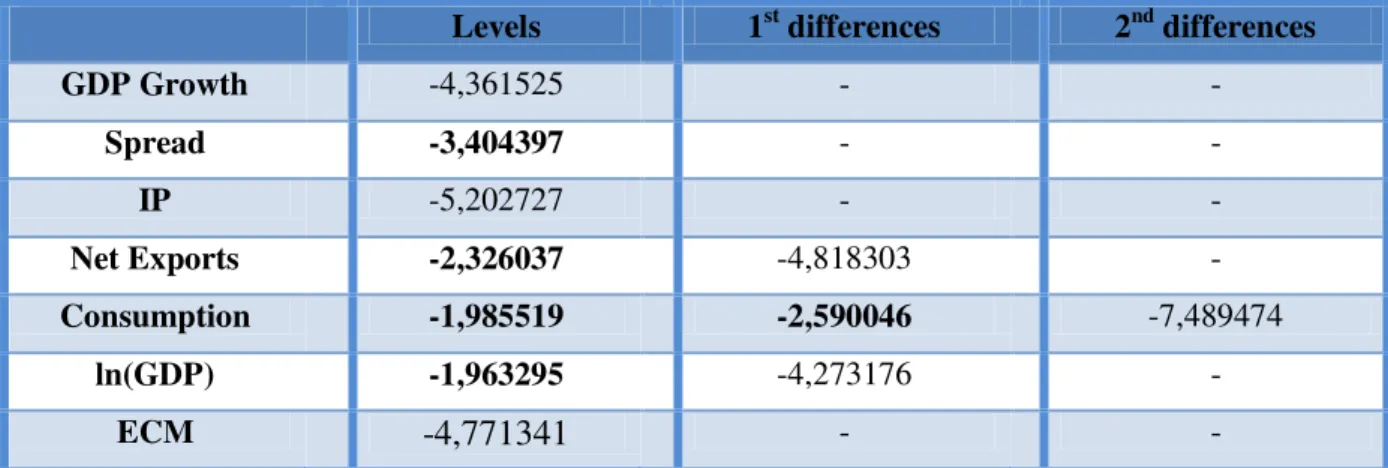
Before performing the econometric exercise, it is important to visually analyze the relationship between real GDP and the two variables considered. From Figure 1 it can be observed that IP and the spread provide leading information for real economic activity in the euro area, suggesting that both variables may help predict GDP growth.

(11)

11

significance, but still because it is very close to the rejection area and we are in the context of the 1% level of significance, the variable will be assumed to be I(0).

4.2 The autoregressive model (AR)

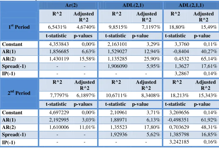
The first model we consider is an AR model of order q, which is normally used as a benchmark in the literature for forecasting comparisons. The decision about the order was made using the AIC and BIC criterion. As summarized in Table 2, the AIC criterion prefers an AR(2) while the BIC criterion prefers an AR(1). Since they give different model choices, I decided to go forward with the AIC as also recommended by Burnham and Anderson (2004).

The intuition behind the AR(2) is that GDP growth can be explained by its past values. From Table 3 and regarding the 1st sub-period we observe that GDP_growtht-1 is statistically significant at the 10% significance level and that GDP_growtht-2 is not significant at any level of significance. Moreover, the constant is statistically significant for all significance levels (p-value is 0). Regarding the 2nd sub-period, GDP_growtht-1 becomes significant at the 5% level and GDP_growtht-2 remains statistically insignificant. Furthermore in the 1st sub-period the R2 is 6,54% and the adjusted R2 is 4,67% and in the 2nd sub-period the R2 is 7,78% and the adjusted R2 is 6,19%.

(12)

12

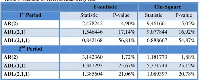
the model and that it is necessary to correct it, otherwise the standard errors, test of significance and inferences may no longer be appropriate. Moreover, when looking at the 2nd sub-period, the model also does not show evidence of autocorrelation (F-statistic is 34,08% and Chi-Square is 32,39%), but there is evidence of heteroscedasticity ( F-statistic is 1,72% and Chi-Square is 1,88%), meaning that we need to correct the AR model also in the 2nd period.

After correcting for the presence of heteroscedasticity, what is most relevant to mention is that in both sub-periods GDP_growtht-2 becomes relevant at a 10% level of significance, as can be seen from Table 6 .

In order to evaluate the out-of-sample results, the static (one step-ahead) forecast method was used. The results for the full period (see Table 9), show that the RMSE is 0,006717, suggesting good forecast accuracy. Moreover, the MAE is 0,003820, confirming the conclusion of the RMSE. Finally, Theil’s Inequality Coefficient, which is scale invariant, is 52,75%, which is quite large and therefore suggesting that the model does not offer a reliable forecast for the data. Besides that, the variance proportion (58,56%) is higher than the covariance proportion (30,34%), indicating that the model is indeed not good in terms of forecasting.

From the beginning of 2008 to 2009 there is a sharp decline that may be affecting the results. Therefore, I decided to analyze the forecasting performance of the model in 2 sub-periods: from 2002q1 to 2006q1 and from 2006q1 to 2009q4. Looking at Table 10, we see that in the 1st sub-period the RMSE decreases to 0,002252, which indicates a better performance, while, if we look at Table 11, in the 2nd sub-period the RMSE increases to 0,009077, indicating a worst performance. Regarding the MAE, the same happens, i.e. in the 1st sub-period it is 0,001844, while in the 2nd sub-period it increases

(13)

13

(23,1%), however the variance proportion remains the highest (53,73%), while in the 2nd sub-period, the value increases (60,67%), having also the variance proportion the highest value (55,15%).

4.3 The Autoregressive Distributed Lag (2,1) Model [ADL]

The second model is an extension of the previous one, where we maintain the AR(2) structure and add lags of the spread variable. Resorting once again to the AIC/ BIC criterion, both point to the inclusion of only one lag of the spread.

(14)

14

In order to validate these conclusions it is necessary to perform as previously. Hence, using robust Breusch-Godfrey tests we test for autocorrelation. From Table 4 we observe that we do not reject the null hypothesis neither in the 1st sub-period (F-statistic is 18,56% and Chi-Square is 16,93%) nor in the 2nd sub-period (F-statistic is 10,26% and the Chi-square is 9,71%, being this last value in the rejection area nevertheless very close to 10% ), which means that there is no autocorrelation in the residuals. Moreover, White’s test for heteroscedasticity (see Table 5), also does not reject the null hypothesis neither in the 1st sub-period (F-statistic is 17,14% and the Chi-Square is 16,92%) nor in the 2nd sub-period (F-statistic is 25,67% and the Chi-Square is 25,12%). We can state, therefore, that this model is autocorrelation and heteroscedasticity free, meaning that previous conclusions can be drawn here as well.

Once again, using the same method (static) and the same forecasting period, the out-of-sample evaluation was conducted. Looking at Table 9, the RMSE is 0,006478, and the MAE is 0,003791. Moreover, Theil’s Inequality coefficient (51,74%) is large, suggesting a bad performance of the model. If we decompose this coefficient, we still have a variance proportion (66,92%) higher than the covariance proportion (22,82%), confirming the previous statement.

(15)

15

and the variance proportion (75,33%) increases, when compared to the full-period, which shows the worse performance of the model in this period.

4.4 The Autoregressive Distributed Lag (2,1,1) Model

The third model is an extension of the previous one, where we maintain the ADL(2,1) structure and add the non-financial variable IP. In this model, both AIC and BIC criterion consider that the best model choice is to include only one lag of IP.

From Table 3, we can see that in both sub-periods only IPt-1 and the constant term are statistically significant at all levels (both variables have p-values close to 0%). All other variables are statistically insignificant. As previously indicated the redundancy test, summarized in Table 7, was conducted in both sub-periods where the GDP_growtht-1, GDP_growtht-2 and Spreadt-1 were considered as the redundant variables. The test allowed to conclude that indeed we do not reject the null hypothesis neither in the 1st sub-period (F-statistic is 41,28% and log likelihood test 39,22%) nor in the 2nd sub-period (F-statistic is 42,34% and the Chi-Square is 40,56%). Despite this conclusion, the variables were not dropped from the model, because non-financial variables should not be used as single predictors but as complementary variables that help improve the prediction exercise (Runstler and Sédillot,2003). Finally, in the 1st sub-period the model presents an R2 of 18,80% and an adjusted R2 of 15,49% and in the 2nd sub-period and R2 of 18,213% and an adjusted R2 of 15,34%.

(16)

16

56,81% and the Chi-Square is 54,87%) nor for the 2nd sub-period (F-statistic is 21,06% and Chi-Square is 20,78%); see Table 5.

Regarding the out-of-sample results, maintaining the static method and the forecasting sample, we can see from Table 9 that the RMSE is 0,006434 and the MAE is 0,004386. Furthermore, the model presents a Theil Inequality coefficient of 45,47%, which, although high, corresponds to the best forecasting model. If we decompose this coefficient, we see that the covariance proportion (68,21%) is the largest and both the bias proportion (13,07%) and the variance proportion (18,72%) are small.

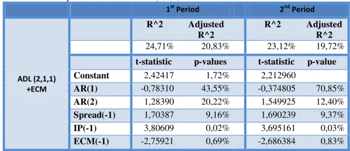
In terms of the sub-periods it follows that in the 1st sub-period (see Table 10) the RMSE (0,002747) and the MAE (0,002234) decrease, showing a better performance of this model in this period, whereas is the 2nd sub-period (see Table 11) both the RMSE (0,008174) and the MAE (0,005973) present a worse performance. Moreover, Theil’s Inequality Coefficient decreases in the 1st sub-period to (26,17%), however this is due to an increase in the bias proportion (30,63%) and a smaller covariance proportion (59,53%) and variance proportion (9,84%), remaining nevertheless a good forecasting model (the covariance proportion is the highest). Regarding the 2nd sub-period, Theil’s Inequality Coefficient increases (50,55%), though there is an increase in the covariance proportion (61,26%) signaling also, that the model is indeed a good forecasting model. 4.4.1 Error Correction Model

The ADL(2,1,1) model by adding IP variable becomes an extension of the ADL(2,1). As a consequence of adding this variable, in terms of in-sample results, the ADL(2,1,1) presents both GDP and spread variables which are statistically insignificant. In order to solve this problem I decided to consider an error correction model.

(17)

17

Table 1, we see that net exports is I(1) and that household consumption requires one differentiation in order to become I(1).

After performing the necessary intermediate stages (e.g. create the residuals and

tests it in order to determine whether cointegration exists) we can conclude that adding the error correction term improves the ADL(2,1,1). In terms of in-sample (see Table 8), the major difference, besides having a statistically significant error correction model, is that the spread becomes statistically significant at a 10% level of significance in both periods and also the adjusted R2 increases in both periods (in the 1st sub-period to 20,83% and in the 2nd sub-period to 19,72%). Moreover, in terms of out-of-sample results, in the full period (see Table 9), there is a decrease of all metrics regarding the ADL(2,1,1) model, which signals a better performance. On the other hand, looking at Tables 10 and 11, it deteriorates its forecasting performance in the 1st sub-period but it improves in the 2nd sub-period.

4.5 Model Comparison

After modeling and forecasting GDP growth through the use of different linear model, a question that can be asked relates to which model performed better in the in-sample and out-of-in-sample period. Previously, the choice of the models was explained, their problems identified and the necessary corrections performed and their forecasts computed. This section will indentify the model that performed better in-sample and out-of-sample.

(18)

18

to be the worse model with an adjusted R2 of 4,67% in the 1st sub-period and 6,19% in the 2nd sub-period.

Concerning the out-of-sample results the metrics used give mixed information. Evaluating first the full sample forecast, the RMSE indicates that the ADL(2,1,1) is the best forecasting model. If we look at the MAE, the ADL(2,1) is considered to be the best. Notice, however, that in terms of Theil’s Inequality Coefficient the ADL(2,1,1) model is not only the best (it has the lowest value of 44,89%) but also the only one that respects the rule that a good forecasting model contains the higher proportion in the covariance.

After splitting the full period into sub-periods, we see that in the 1st sub-period the autoregressive model clearly performs better in all metrics, nevertheless, the ADL(2,1,1) is the only one that respects the rule of having the covariance proportion higher than the other proportions. Regarding the 2nd sub-period, the autoregressive model becomes the worst model, whereas if we use the MAE, the best model is the ADL(1,1) (disregarding ADL(2,1,1) with the error term, otherwise it would be this one), while if we use the RMSE and the Theil Inequality Coefficient the best is ADL(2,1,1).

5 Conclusion

The goal of this paper was to model GDP growth in the euro area through the use of 3 types of models: an AR model, an ADL(2,1) model (comprehending the autoregressive component and the term spread) and an ADL(2,1,1) (a three variables model with GDP, term spread and IP). The analyses of each model was conducted both in-sample and out-of-sample.

(19)

19

the only model that respects the rule of having a covariance proportion in Theil’s Inequality Coefficient higher than the other proportion in every period evaluated. Moreover, the AR model outperforms the others if we reduce the forecasting period to 2002q1 to 2006q1. In the period of 2006q1 to 2009q4 the best model can be either the ADL(2,1,1) or the ADL(2,1), depending on the metrics used.

The main limitation of this analysis arises from the data issue of aggregate versus disaggregated data. This study focuses on aggregated data for the euro area. Despite the potential benefits of disaggregated data approaches based on the aggregation of individual countries, the evidence about this subject is still quite mixed. For example, Marcellino et al (2003) concluded that forecasts from disaggregated data, in general,

outperform those from aggregate data, nevertheless as argued by Baffigi et al (2002),

these gains depend on the properties of the single country specifications and may vary over the forecast horizon.

Another caveat is the linear framework developed throughout the paper. Indeed, the results obtained are taken from a setting of linear models and therefore the analysis should be interpreted in that context. It is possible that financial variables have a nonlinear impact on macroeconomic variables and consequently that impact should be modeled by a nonlinear regression. Nevertheless, as stated by Marcellino (2007: abstract): “Our main conclusion is that in general linear time series models can be hardly beaten if they are carefully specified”.

(20)

20

6 References

Baffigi, A., Golinelli, R., and Parigi, Giussepe. 2002. "Real-time GDP forecasting in the euro area." Bank of Italy Economic Research Paper No 456.

Banerjee, A., I. Masten, and Massimiliano Marcellino. 2003. “Leading indicators

for euro area inflation and GDP growth.” Oxford Bulletin of Economics and Statistics,

Vol. 67:785-813.

Banerjee, A., and Massimiliano Marcelino. 2005. “Are there any reliable leading indicators for the US inflation and GDP growth?”International Journal of Forecasting.

Burnham, K. P., and David R. Anderson. (2004). "Multimodel inference: understanding AIC and BIC in Model Selection." Sociological Methods and Research, 33: 261-304.

Dotsey, Michael. 1998. “The Predictive Content of the Interest Rate Term Spread for Future Economic Growth.” Federal Reserve Bank of Richmond Economic Quarterly 84.

Duarte, A., I. A.Venetis and Ivan Paya. 2005. “Predicting real growth and the

probability of recession in the Euro area using the yield spread.” Instituto Valenciano de Investigaciones Económicas Discussion Paper 31.

Espinoza, R., Fabio Fornari, and Marco J. Lombardi. 2009. “The role of financial variables in predicting economic activity.” ECB Working Paper 1108.

Estrella, Arturo, and Gikas A Hardouvelis. 1991. “The term structure as a predictor of real economic activity.”Journal of Finance, Vol. 46 No 2.

Estrella, Arturo, and Frederic Mishkin. (1996). “Predicting U.S recessions: Financial variables as leading Indicators.” NBER Working Paper 5379.

Hamilton, J., and Doeng Heon Kim. 2002. “A re-examination of the predictability of economic activity using the yield spread.” Journal of Money, Credit and Banking,

(21)

21

Harvey, Campbell. 1997. “The relation between the term structure of interest rates

and Canadian economic growth.” Canadian Journal of Economics, Vol. 30: 169—93.

Haubrich, J.G., and Ann M. Dombrosky. 1996. “Predicting Real Growth Using

the Yield Curve.” Federal Reserve Bank of Cleveland Economic Review 32 (1): 26 – 34.

Koenig, Evan, and Kenneth M. Emery . 1991. “Misleading Indicators? Using the Composite Leading indicators to predict cyclical turning points.” Federal Reserve Bank of Dallas Economic Review 1991-jul: 1-14.

Marcellino, Massimiliano. 2007. “A comparison of time series models for

forecasting GDP growth and inflation.” IEP – Università Bocconi, IGIER and CEPR. Marcellino, M., Jame H. Stock, and Mark W. Watson. 2003. “Macroeconomic Forecasting in the Euro-Area: Country Specific versus Euro-Area Information.” IGIER – Università Bocconi Working Paper 201.

Moneta, Fabio. 2005. “Does the yield spread predict recessions in the euro-area?”

International Finance, Vol. 8(2): 263-301.

Plosser, Charles, and K. Geert Rouwenhorst. 1994. “International term structures

and real economic growth.” Journal of Monetary Economics, Vol. 33: 33-55.

Rϋnstler, Gerhard, and Franck. Sédillot. 2003. “Short-Term Estimates of Euro Area Real GDP by Means of Monthly Data.” ECB Working Paper No. 276.

Stock, James, and Mark W. Watson. 2001. “Forecasting Output and Inflation: The role of asset prices.” NBER Working Paper 8180

(22)

22

7 Appendices

Figure 1: Growth rates of GDP, Spread and Industrial Production

Table 1: ADF test

Levels 1st differences 2nd differences

GDP Growth -4,361525 - -

Spread -3,404397 - -

IP -5,202727 - -

Net Exports -2,326037 -4,818303 -

Consumption -1,985519 -2,590046 -7,489474

ln(GDP) -1,963295 -4,273176 -

ECM -4,771341 - -

Table 2: Models Order Choice

Autoregressive ADL(2,q) ADL(2,1,m)

AIC BIC AIC BIC AIC BIC

AR(1)

-7,648332

-7,597478 Spread(-1)

-7,679110

-7,576170 IP(-1) -7,783005 -7,654330

AR(2)

-7,670988

-7,594249 Spread(-2)

-7,660037

-7,530575 IP(-2) -7,773657 -7,618303

AR(3)

-7,659188

-7,556248 Spread(-3)

-7,648480

-7,492170 IP(-3) -7,763301 -7,580939

AR(4)

-7,644446

-7,514984 Spread(-4)

-7,632755

-7,449262 IP(-4) -7,750993 -7,541286

AR(5)

-7,662062

-7,505752 Spread(-5)

-7,629421

-7,418403 IP(-5) -7,741629 -7,504234

AR(6)

-7,640189

-7,456696 Spread(-6)

-7,605833

-7,366943 IP(-6) -7,734653 -7,469219

-0. 12 -0. 08 -0. 04 0. 00 0. 04 0. 08

80 85 90 95 00 05

(23)

23

Table 3: In-sample results

1st Period

Ar(2) ADL(2,1) ADL(2,1,1)

R^2 Adjusted R^2

R^2 Adjusted R^2 6,5431% 4,6740% 9,8515% 7,1197% 18,80% 15,49% t-statistic p-values t-statistic p-value t-statistic p-value

Constant 4,353843 0,00% 2,163101 3,29% 3,3760 0,11%

AR(1) 1,856685 6,63% 1,529027 12,94% -0,8404 40,27%

AR(2) 1,430119 15,58% 1,135285 25,90% 0,4532 65,14%

Spread(-1) - - 1,906090 5,95% 1,3627 17,61%

IP(-1) - - - - 3,2867 0,14%

2nd Period

R^2 Adjusted R^2

R^2 Adjusted R^2 7,7797% 6,1897% 10,6711% 8,3408% 18,213% 15,343% t-statistic p-values t-statistic p-value t-statistic p-value

Constant 4,697229 0,00% 2,10961 3,71% 3,269656 0,14%

AR(1) 2,192995 3,03% 1,88971 6,13% -0,498351 61,92%

AR(2) 1,610006 11,01% 1,35523 17,80% 0,703629 48,31%

Spread(-1) - - 1,92936 5,62% 1,385798 16,85%

IP(-1) - - - - 3,242185 0,16%

Table 4: Results of Autocorrelation test

F-statistic Chi-Square

1st Period Statistic P-value Statistic P-value

AR(2) of order 4 1,035760 39,29% 4,261237 37,18%

ADL(2,1) of order 4 1,581077 18,56% 6,4289 16,93%

ADL (2,1,1) of order 4 1,864026 12,32% 7,569566 10,87%

2nd Period

AR(2) of order 4 1,141397 34,08% 4,660937 32,39%

ADL(1,1) of order 4 1,978329 10,26% 7,853543 9,71%

(24)

24

Table 5: Results of Heteroscedasticity test

F-statistic Chi-Square

1st Period Statistic P-value Statistic P-value

AR(2) 2,478242 4,90% 9,461661 5,05%

ADL(2,1) 1,546446 17,14% 9,077844 16,92%

ADL(2,1,1) 0,842168 56,81% 6,888667 54,87%

2nd Period

AR(2) 3,142360 1,72% 1,181773 1,88%

ADL(1,1) 1,347293 25,67% 5,371749 25,12%

ADL(2,1,1) 1,385604 21,06% 1,089397 20,78%

Table 6: Corrected output

1st Period 2nd Period t-statistic p-values t-statistic p-values

AR Model

Constant 3,815884 0,02% 4,217350 0,00%

AR(1) 1,834028 6,96% 2,133458 3,50%

AR(2) 1,727804 8,71% 1,865716 6,46%

ADL (1,1) Model

Constant - - 2,334231 2,13%

AR(1) - - 2,298947 2,33%

Spread (-1) - - 2,470853 1,49%

R^2 Adjusted

R^2

R^2 Adjusted R^2

- - 10,93% 9,41%

Table 7: Results of Redundant Test

F-statistic Log Likelihood

ratio 1st Period Statistic P-value Statistic P-value ADL(2,1) Model 2,217886 11,42% 4,514594 10,46% ADL(2,1,1) Model 0,964336 41,28% 2,996594 39,22%

2nd Period

(25)

25

Table 8: In-sample Results for the ADL(1,1,2) with Error Correction Model 1st Period 2nd Period

ADL (2,1,1) +ECM

R^2 Adjusted R^2

24,71% 20,83% 23,12% 19,72%

t-statistic p-values t-statistic p-value

Constant 2,42417 1,72% 2,212960

AR(1) -0,78310 43,55% -0,374805 70,85%

AR(2) 1,28390 20,22% 1,549925 12,40%

Spread(-1) 1,70387 9,16% 1,690239 9,37%

IP(-1) 3,80609 0,02% 3,695161 0,03%

ECM(-1) -2,75921 0,69% -2,686384 0,83%

Table 9: Out-of-sample results for the full period

AR(2) ADL(2,1) ADL(2,1,1) ADL(2,1,1)+ECM

RMSE 0,006717 0,006539 0,006183 0,00541

MAE 0,00382 0,003772 0,004135 0,00394

Theil Inequality C. 52,755% 52,172% 44,885% 38,233%

Bias Proportion 11,095% 10,830% 12,571% 3,781%

Variance Proportion 58,564% 69,393% 26,617% 10,365%

Covariance Proportion 30,341% 19,777% 60,812% 85,854%

Table 10: Out-of-sample results for the 1st sub-period

AR(2) ADL(2,1) ADL(2,1,1) ADL(2,1,1)+ECM

RMSE 0,002252 0,002412 0,002747 0,00304

MAE 0,001844 0,001977 0,002234 0,00245

Theil Inequality Coefficient

23,099% 24,109% 26,168% 27,755%

Bias Proportion 16,199% 23,513% 30,629% 40,508%

Covariance Proportion 30,069% 27,380% 59,527% 55,156%

Table 11: Out-of-sample results for the 2nd sub-period

AR(2) ADL(2,1) ADL(2,1,1) ADL(2,1,1)+ECM

RMSE 0,009077 0,00884 0,008174 0,006977

MAE 0,005843 0,005565 0,005973 0,005431

Theil Inequality Coefficient

60,673% 62,129% 50,547% 42,510%

Bias Proportion 11,714% 10,405% 8,523% 0,005%

(26)

NOVA SCHOOL OF BUSINESS AND ECONOMICS

Appendix

Time Series’ concepts and Eviews’ Outputs

Cláudia Campos

07-01-2013

A project carried out on the Corporate Finance Major, under the supervision of: Paulo M. M. Rodrigues

(27)

2

Index

1 Time Series Concepts ...4

1.1 The Classical Linear Regression Model ...4

1.1.1 Whites’ Heteroscedasticity test ...4

1.1.2 Breusch-Godfrey’s Autocorrelation test ...5

1.2 The Autoregressive (AR) model of order p ...6

1.3 Autoregressive Distributed Lag Model of order (p,q,m) ...6

1.4 Cointegration ...7

1.4.1 Unit root tests ...8

1.4.2 Error Correction Model ...8

1.4.3 The Engle Granger test ...9

1.5 T-statistics and P-values ...9

1.5.1 Redundant Test ...10

1.6 F-test...10

1.7 Goodness of Fit Statistic ...11

2 _{Eviews’ Outputs} ...12

2.1 ADF test in levels ...12

2.1.1 GDP growth variable ...12

2.1.2 Spread variable ...13

2.1.3 IP growth variable ...14

2.1.4 Net Exports variable ...15

2.1.5 Household Consumption variable ...17

2.1.6 GDP variable ...20

2.1.7 ECM ...22

2.2 Order Selection ...23

2.2.1 AR ...23

2.2.2 ADL(2,q) ...26

2.2.3 ADL(2,1,m) ...31

2.3 Model tests ...35

2.3.1 AR(2) 1st_sub-period_...35

2.3.2 AR(2) 2nd_sub-period

...37

2.3.3 ADL(2,1) 1st_sub-period_...38

2.3.4 ADL(1,1) 2nd sub-period ...39

(28)

3

2.3.6 ADL(2,1,1) 2nd_sub-period

...42

2.3.7 ADL(2,1,1) plus the Error Correction Model ...43

2.4 Out-of-sample results ...45

2.4.1 AR(2)...45

2.4.2 ADL(2,1) ...46

2.4.3 ADL(2,1,1) ...47

(29)

4

1 Time Series Concepts

1.1The Classical Linear Regression Model

The multiple linear regression model is a generalization of the simple model and has the following expression:

(1) In order to obtain the parameter estimates, the Residual Sum of Squares has to be minimized with respect to all the βs. Typically the following assumptions needed to be consider for the Multiple Linear Regression Model to be valid:

1.

2. (Homoscedasticity) 3. (No autocorrelation)

4. (No relationship between error and corresponding x variate) 5. (this assumption is required if we want to make inferences about the population parameters from the sample parameters)

If some of the assumptions do not hold, a combination of the following problems may occur: coefficient estimates may be wrong, associated standard errors may be wrong and the distribution assumed for the test statistic inappropriate. So it becomes relevant to test these assumptions in order to validate the model.

After estimating the models the following tests are necessary to perform in order to ensure that the assumptions hold:

1.1.1 Whites’ Heteroscedasticity test

(30)

5

For example, if we considered the initial regression with 3 independent variables,

White’s auxiliary regression would be,

(2)

Hence, in order for the errors to be homoscedastic, the i, i = 1,…,6 have to equal 0. Therefore, the null hypothesis is and the alternative .

The test statistic for heteroscedasticity is which under the hull hypothesis converges to a Chi-square distribution with k degrees of freedmon. If the test statistic is above the corresponding critical value, we reject the null hypothesis of homocedasticity. The coefficient estimates are still unbiased, but the standard errors, tests of significance and inferences may no longer be appropriate.

In order to correct for heteroscedasticity, White’s robust standard errors can be used.

1.1.2 Breusch-Godfrey’s Autocorrelation test

The Breusch-Godfrey test allows testing for autocorrelation of order q. Considering a linear regression model with m explanatory variables, the following auxiliary regression will have to be computed,

(3)

where correspond to the regression residuals.

In order for the errors not to be autocorrelated, the s have to equal 0. Therefore, the null hypothesis is and the alternative .

The test statistic for autocorrelation of order k is which under the hull hypothesis converges to a Chi-square distribution with k degrees of freedom.

(31)

6

(4)

1.2 The Autoregressive (AR) model of order p

(5) An AR(p) process is a process where the present values of the variable depend solely on the past values of the variable that we want to analyze plus a random error term (such as white noise). Notice that measures the persistence of the past values of the dependent variable.

The above expression is normally written in terms of the lag operator, moving all lags of the dependent variables to the LHS, i.e.

(6) Or equivalently:

(7) Where β is a polynomial in the lag operator and β the coefficients. The lag operator is important because it allows simplifying the notation of the time series model. This model is important because it is used as the benchmark to compare with the other models proposed.

1.3 Autoregressive Distributed Lag Model of order (p,q,m)

(32)

7

Where , and are stationary variables, ut is white noise and p,q,m represent the number of lags of the correspondent variable.

In type of model, the concept of white noise is very important. By definition, ut is white noise if each value in the sequence has zero mean, a constant variance and it is serially uncorrelated:

(9)

(10)

for all u (11) If the error term is indeed white noise process (more generally it is stationary and independent of yt and Xt’s variables), the ADL model can be estimated consistently with by ordinary least squares.

1.4 Cointegration

In most cases, if two variables that are I(1) are linearly combined, the combination will also be I(1). It can be generalize that if variables with differing orders of integration are combined, then the combination will have an order of integration equal to the largest.

In general, many financial variables contain at least one unit root. In this context, a set of variables is defined as cointegrated if a linear combination of them is stationary. Many time series are non-stationary nevertheless the variables may “move together”

over time (i.e there is some influences on the series, which implies that the two series

(33)

8 1.4.1 Unit root tests

Unit root tests are used to determine whether a series is stationary [I(0)] or not [superior orders of I(d)]. A formal procedure that can be used in this context is the Augmented Dickey Fuller test (ADF).

There are three versions of the ADF test:

(12)

(13)

(14) where (12) is ADF with no constant nor trend; (13) is ADF with constant and no trend and (14) is ADF with constant and trend.

This test aims to test the null hypothesis, =0, of a unit root. The augmented version of the Dickey Fuller test varies from the original model by including extra lags of the dependent variable with the objective to ensure that the residuals are autocorrelation free.

1.4.2 Error Correction Model

One way to correct for the non-stationary is to take the 1st differences, however the problem with this approach is that the pure 1st differenced model have no long-run solution. For example, considering and both I(1):

(15)

This has no long-run solution. One way to correct such problem is to use the first differences and level terms, e.g.:

(34)

9

Where is known as the error correction term. This error term will be I(0), even knowing that both variables are I(1).

1.4.3 The Engle Granger test

The Engle and Granger test is used to test for cointegration. In other words,

In order to perform this test two steps are require. First, each variable is tested using the ADF in order to make sure that they are I(1), then the cointegration regression is estimated using OLS and the residuals of such a regression saved. Then, to conclude step 1, using ADF we test the residuals saved to ensure that they are I(0). However, because this is a test on the residuals of an actual model the critical values are different. The 2nd step consists on using the residuals of step 1 as one variable in the error correction model e.g.

(17) where

(18)

1.5 T-statistics and P-values

The t-statistic is used when we want to test if the true value of the parameter is a given value (β ).

β β

(35)

10

The p-value is the maximum significance level at which we do not reject the null hypothesis.

In the case that the variables are statistically insignificant, the redundant test should be performed:

1.5.1 Redundant Test

This test is used to determine whether a variable is irrelevant or not for a given model. In this test we compare the original model with the model without the statistically insignificant variables. For example, considering the following regression:

(20) and assume that β is statistically insignificant. Hence, we run the following restricted regression:

(21) The test compares the values of R2 for the 2 models (F-test) and the value of the log-likelihood of the 2 models (Likelihood-Ratio test). The consequence of including an irrelevant variable would be that the coefficient estimators would still be consistent and unbiased, but no longer efficient. As a consequence, the standard errors for the coefficients are likely to be inflated relative to the values which they would have taken in the case of not including the irrelevant variable.

1.6 F-test

(36)

11 1.7 Goodness of Fit Statistic

The classical goodness of fit statistics is,

(22) This statistic indicates the percentage of the behavior of the dependent variable explained by the regression and therefore can be seen as an in-sample comparison measure. However, if we increase the number of regressors in the model, the will also increase, although the fit may not improve in a practical sense. Therefore, the comparison between models has to be made using the adjusted ( ), which penalizes the goodness of fit when extra variables are added, taking into account the loss of degrees of freedom. Meaning that in order for to increase, has to increase sufficiently to compensate for the added variables, i.e.,

(37)

12

2 Eviews

’

Outputs

2.1 ADF test in levels 2.1.1 GDP growth variable

ADF Test Statistic -4.361525 1% Critical Value* -3.4807 5% Critical Value -2.8833 10% Critical Value -2.5783 *MacKinnon critical values for rejection of hypothesis of a unit root.

Augmented Dickey-Fuller Test Equation Dependent Variable: D(GDP_GROWTH) Method: Least Squares

Date: 11/09/12 Time: 10:46 Sample(adjusted): 1977:1 2009:4

Included observations: 132 after adjusting endpoints

Variable Coefficient Std. Error t-Statistic Prob.

GDP_GROWTH(-1) -0.566045 0.129781 -4.361525 0.0000

D(GDP_GROWTH(-1)) -0.086642 0.132104 -0.655860 0.5131

D(GDP_GROWTH(-2)) 0.012233 0.128395 0.095280 0.9242

D(GDP_GROWTH(-3)) 0.059071 0.126967 0.465248 0.6426

D(GDP_GROWTH(-4)) 0.143041 0.101380 1.410945 0.1607

C 0.002724 0.000835 3.262831 0.0014

R-squared 0.331237 Mean dependent var -0.000111

Adjusted R-squared 0.304699 S.D. dependent var 0.006540 S.E. of regression 0.005453 Akaike info criterion -7.540780 Sum squared resid 0.003747 Schwarz criterion -7.409743

Log likelihood 503.6915 F-statistic 12.48152

(38)

13 2.1.2 Spread variable

Augmented Dickey-Fuller Test Equation Dependent Variable: D(SPREAD) Method: Least Squares

SPREAD(-1) -0.168396 0.049464 -3.404397 0.0009

D(SPREAD(-1)) 0.091932 0.088721 1.036199 0.3021

D(SPREAD(-2)) 0.095557 0.081796 1.168239 0.2449

D(SPREAD(-3)) -0.121777 0.082379 -1.478249 0.1418

D(SPREAD(-4)) 0.171877 0.084781 2.027312 0.0447

C 0.003227 0.001065 3.031262 0.0030

R-squared 0.145310 Mean dependent var -4.51E-05

(39)

14 2.1.3 IP growth variable

Augmented Dickey-Fuller Test Equation Dependent Variable: D(IP)

Method: Least Squares Date: 11/09/12 Time: 11:05 Sample(adjusted): 1977:1 2009:4

IP(-1) -0.704825 0.135472 -5.202727 0.0000

D(IP(-1)) 0.243853 0.126486 1.927905 0.0561

D(IP(-2)) 0.192193 0.124767 1.540414 0.1260

D(IP(-3)) 0.191162 0.139481 1.370519 0.1730

D(IP(-4)) 0.148943 0.116986 1.273174 0.2053

C 0.002223 0.001267 1.755074 0.0817

(40)

15 2.1.4 Net Exports variable

2.1.4.1 Level

Augmented Dickey-Fuller Test Equation Dependent Variable: D(LNETEX) Method: Least Squares

LNETEX(-1) -0.110873 0.047666 -2.326037 0.0216

D(LNETEX(-1)) -0.341667 0.090552 -3.773157 0.0002

D(LNETEX(-2)) 0.046680 0.094984 0.491450 0.6240

D(LNETEX(-3)) 0.031727 0.094741 0.334882 0.7383

D(LNETEX(-4)) -0.095407 0.087322 -1.092586 0.2767

C 1.104406 0.464995 2.375094 0.0191

R-squared 0.213417 Mean dependent var 0.017411

Adjusted R-squared 0.182203 S.D. dependent var 0.581818 S.E. of regression 0.526150 Akaike info criterion 1.597928 Sum squared resid 34.88105 Schwarz criterion 1.728964

Log likelihood -99.46325 F-statistic 6.837305

(41)

16

2.1.4.2 1st Diferences

Augmented Dickey-Fuller Test Equation Dependent Variable: D(LNETEX.2) Method: Least Squares

D(LNETEX(-1)) -1.243558 0.258091 -4.818303 0.0000

D(LNETEX(-1).2) -0.145318 0.225970 -0.643088 0.5213

D(LNETEX(-2).2) -0.151509 0.190984 -0.793309 0.4291

D(LNETEX(-3).2) -0.172721 0.149181 -1.157793 0.2492

D(LNETEX(-4).2) -0.213399 0.087075 -2.450752 0.0156

C 0.014701 0.045929 0.320085 0.7494

Adjusted R-squared 0.715943 S.D. dependent var 0.979888 S.E. of regression 0.522250 Akaike info criterion 1.583380

Sum squared resid 34.09318 Schwarz criterion 1.715069

Log likelihood -97.71140 F-statistic 66.53104

(42)

17 2.1.5 Household Consumption variable

2.1.5.1 Level

Augmented Dickey-Fuller Test Equation Dependent Variable: D(LCONS)

LCONS(-1) -0.044485 0.022405 -1.985519 0.0493

D(LCONS(-1)) 0.007061 0.086599 0.081538 0.9351

D(LCONS(-2)) 0.183147 0.085358 2.145648 0.0338

D(LCONS(-3)) 0.246705 0.086681 2.846128 0.0052

D(LCONS(-4)) 0.268007 0.088732 3.020406 0.0031

C 0.587376 0.294394 1.995202 0.0482

@TREND(1975:4) 0.000224 0.000120 1.870095 0.0638

(43)

18

Augmented Dickey-Fuller Test Equation Dependent Variable: D(LCONS,2) Method: Least Squares

D(LCONS(-1)) -0.372929 0.143986 -2.590046 0.0107

D(LCONS(-1),2) -0.662058 0.148587 -4.455693 0.0000

D(LCONS(-2),2) -0.531801 0.146030 -3.641736 0.0004

D(LCONS(-3),2) -0.342239 0.129070 -2.651578 0.0091

D(LCONS(-4),2) -0.100141 0.090695 -1.104148 0.2717

C 0.002629 0.001339 1.963904 0.0518

@TREND(1975:4) -1.36E-05 1.19E-05 -1.144949 0.2544

(44)

19

2.1.5.3 2nd Diferences

Augmented Dickey-Fuller Test Equation Dependent Variable: D(LCONS,3) Method: Least Squares

D(LCONS(-1),2) -3.484549 0.465260 -7.489474 0.0000

D(LCONS(-1),3) 1.512888 0.410295 3.687315 0.0003

D(LCONS(-2),3) 0.735974 0.314416 2.340763 0.0209

D(LCONS(-3),3) 0.222503 0.200181 1.111508 0.2685

D(LCONS(-4),3) 0.029400 0.090114 0.326248 0.7448

C -4.94E-05 0.000948 -0.052081 0.9585

@TREND(1975:4) -2.84E-06 1.18E-05 -0.240932 0.8100

Adjusted R-squared 0.832967 S.D. dependent var 0.012288 S.E. of regression 0.005022 Akaike info criterion -7.697613

Sum squared resid 0.003102 Schwarz criterion -7.543207

(45)

20 2.1.6 GDP variable

2.1.6.1 Level

Augmented Dickey-Fuller Test Equation Dependent Variable: D(LGDP)

LGDP(-1) -0.058216 0.029652 -1.963295 0.0518

D(LGDP(-1)) 0.359297 0.088419 4.063573 0.0001

D(LGDP(-2)) 0.128858 0.094963 1.356923 0.1773

D(LGDP(-3)) 0.074193 0.096564 0.768329 0.4437

D(LGDP(-4)) 0.098513 0.100072 0.984420 0.3268

C 0.799899 0.405743 1.971440 0.0509

@TREND(1975:4) 0.000307 0.000163 1.878276 0.0627

Adjusted R-squared 0.167917 S.D. dependent var 0.005935 S.E. of regression 0.005414 Akaike info criterion -7.548209

Sum squared resid 0.003663 Schwarz criterion -7.395333

(46)

21

Augmented Dickey-Fuller Test Equation Dependent Variable: D(LGDP,2)

D(LGDP(-1)) -0.579296 0.135566 -4.273176 0.0000

D(LGDP(-1),2) -0.070282 0.134587 -0.522202 0.6025

D(LGDP(-2),2) 0.014170 0.130455 0.108621 0.9137

D(LGDP(-3),2) 0.055032 0.127983 0.429994 0.6679

D(LGDP(-4),2) 0.146418 0.101325 1.445030 0.1510

C 0.003925 0.001370 2.865034 0.0049

@TREND(1975:4) -1.54E-05 1.30E-05 -1.186878 0.2375

(47)

22 2.1.7 ECM

2.1.7.1 Level

Augmented Dickey-Fuller Test Equation Dependent Variable: D(ECM)

ECM(-1) -0.314930 0.066004 -4.771341 0.0000

D(ECM(-1)) 0.161301 0.089639 1.799458 0.0743

D(ECM(-2)) 0.176010 0.086719 2.029652 0.0445

D(ECM(-3)) 0.001541 0.087904 0.017527 0.9860

D(ECM(-4)) 0.229397 0.092498 2.480030 0.0144

(48)

23 2.2 Order Selection

2.2.1 AR

2.2.1.1 AR(1)

Dependent Variable: GDP_GROWTH Method: Least Squares

Included observations: 104 after adjusting endpoints Convergence achieved after 2 iterations

Newey-West HAC Standard Errors & Covariance (lag truncation=4)

C 0.005859 0.000723 8.100563 0.0000

GDP_GROWTH(-1) 0.226559 0.118518 1.911601 0.0587

Durbin-Watson stat 2.057179 Prob(F-statistic) 0.020743 Inverted AR Roots .23

2.2.1.2 AR(2)

C 0.005697 0.000756 7.539993 0.0000

GDP_GROWTH(-1) 0.181269 0.098837 1.834028 0.0696

GDP_GROWTH(-2) 0.139790 0.080906 1.727804 0.0871

(49)

24

2.2.1.3 AR(3)

C 0.005583 0.000839 6.651994 0.0000

GDP_GROWTH(-1) 0.151805 0.100190 1.515167 0.1329

GDP_GROWTH(-2) 0.117845 0.083681 1.408263 0.1622

GDP_GROWTH(-3) 0.098667 0.099018 0.996452 0.3215

Durbin-Watson stat 2.021045 Prob(F-statistic) 0.081309 Inverted AR Roots .61 -.23 -.33i -.23+.33i

2.2.1.4 AR(4)

C 0.005508 0.000944 5.832153 0.0000

GDP_GROWTH(-1) 0.138894 0.107117 1.296661 0.1979

GDP_GROWTH(-2) 0.102355 0.086189 1.187559 0.2379

GDP_GROWTH(-3) 0.077157 0.111407 0.692563 0.4903

GDP_GROWTH(-4) 0.123261 0.144561 0.852659 0.3960

(50)

25

2.2.1.5 AR(5)

C 0.005495 0.000774 7.100482 0.0000

GDP_GROWTH(-1) 0.157842 0.101210 1.559552 0.1222

GDP_GROWTH(-2) 0.101109 0.087333 1.157749 0.2499

GDP_GROWTH(-3) 0.068641 0.111638 0.614853 0.5401

GDP_GROWTH(-4) 0.141836 0.141381 1.003222 0.3183

GDP_GROWTH(-5) -0.146734 0.071380 -2.055678 0.0426

Durbin-Watson stat 1.952609 Prob(F-statistic) 0.121916 Inverted AR Roots .59 -.23i .59+.23i -.15+.69i -.15 -.69i