“EXTERNAL SUSTAINABILITY ANALYSIS: CYCLICAL VERSUS NON-CYCLICAL CURRENT ACCOUNT BALANCES IN THE EUROZONE”
TAMARA TINTI – 2451
A Project carried out on the Master in Finance Program, under the supervision of: Professor Francesco Franco
2
“External Sustainability Analysis: Cyclical Versus Non-Cyclical Current Account Balances in the Eurozone”
ABSTRACT
The persistent widening phase of current account balances1 recorded in the last years has sharply reversed during the crisis of 2008. In order to predict their future evolution, it is fairly necessary to identify both structural and cyclical factors and understand in which way they could affect the imbalances. The purpose of this paper is to determine the existing link between these components using a panel of 28 European countries from 1972 and 2014. We found that a major contribution on those balances is provided in large part by structural factors.
Keywords: Current account; global imbalances; Euro-area; panel estimation
Research question: How important are the explicative variables for the current account balances? A possible answer is provided in this paper via a panel-econometric estimation on the most common determinants of current account balances.
1
3
Introduction
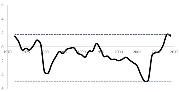
The 2008 financial crisis has lead to a deep fall in the EU28 current account (CA) balances, up to a deficit of 5% of the GDP. This represented the worst situation after the negative values reported during the oil crisis of 1980 and the dot-com bubble of late 1990s, whose amounts (as shown in Figure 1) were respectively -4% and -2%.
Figure 1. European (28 countries) Current Account Balance (% of GDP), 1972 – 2014
Although the picture depicted above represents the overall European situation, the actual scenario is quite various. Several reasons of this heterogeneity were identified by the European Commission, on both European and international levels. Low interest rates have led to a rise in investors’ risk appetite and, in turn, to a credit risk underpricing and a global credit boom. Further, with the expansion in global trade and the steep growth of emerging economies, markets faced an increase in their size and the whole Euro-Area received the competitive pressures from those new players.
Generally, more developed (core) countries have large and persistent surpluses, as happen in Germany, the Netherlands, Sweden and Denmark. Conversely, catch-up (peripheral) countries
-6 -4 -2 0 2 4 6
1970 1975 1980 1985 1990 1995 2000 2005 2010 2015
4
show large deficits. Traditionally, those peripheral deficits are associated with a weak growth process, unable to stimulate the appropriate rebalancing, and lack in competitiveness that could be improved through labour market reforms with the main purpose of raising their productivity. This dualism is even more evident by comparing pre- and post-crisis periods: Between 1990 and 2007, the balances had widened, since surpluses increased meanwhile deficits deteriorated; then, after 2008, those balances have narrowed thanks to a correction of deficits, showing nowadays a sizable surplus. However, those imbalances’ corrections occurred only after the severe problems emerged with the sovereign debt crisis and at a slower pace. As suggested by Deutsche Bundesbank, since those countries belong to a Monetary Union, the implemented mechanism could not rely on the exchange rate adjustments2, as happened during the oil crisis or in economies with different exchange regimes, neither on the interest rate flexibility. Thus, the rebalancing process in countries joining a Monetary Union figures to be the slowest one. Moreover, if the determinants driving these current account changes were transitory, these imbalances would likely record another widening phase in the medium-term. Conversely, if the nature of those factors is purely structural, the improvement in the imbalances will be expected to be persistent over time. Hence, the purpose of this paper is to investigate which are the medium-term determinants of the current account balances, both in structural and cyclical terms, and their explicative power, estimating this relationship via a panel-econometric model.
The analysis is firstly based on replicating a Bruegel Working Paper (by Zsolt Darvas3), with a specific focus on the European context, pointing out the explicability power of the variables
2
Friedman (1953) suggested that the exchange rate regime is a fundamental element in the current account adjustment process.
Friedman, Milton. 1953. “The Case for Flexible Exchange Rates”. Essays in Positive Economics. University of Chicago Press. 157-203.
3
5
considered and the weaknesses of this model specification. Secondly, the model is extended to include new current account determinants in order to figure out if those additional control variables could help in better explaining the existing relation. Finally, both models and their results are compared.
Current account balances: Review of the empirical literature
Although the vast heterogeneity of the Euro-Area and the overall current account balance, many researches have demonstrated that all those countries share similar weaknesses. Hence, some attention should be paid on both deficit and surplus countries: The former show low level of debt sustainability and competitiveness, whereas the latter can hide other kind of economic and/or financial vulnerabilities.
6
imposed by a weak institutional system, low levels of growth are expected to be recorded in the following years. Finally, a smaller contribution is also given by shortcomings in the public administration, energy and transportation sectors.
In order to solve the weaknesses highlighted above, the European Commission suggested to improve competitiveness and productivity, enhancing the country’s long-term sustainability via a strong process of reforms. In this direction, an empirical research4 has evidenced the good results obtained in the German current account: Labour market liberalisation reforms and a specific focus on exports boosted competitiveness and, thus, the German surplus. Further, to address the failures introduced above and enhance domestic demand, surplus countries should invest in adopting an appropriate financial regulation and macro-prudential supervision. In addition, in past years, an initial adjustment phase started through the reduction in private domestic demand, while the most recent balances are achieved through export growth. At the same time, although the adjustment process already done, the European Commission5 suggests an important challenge: Both peripheral and core countries require capital inflows, mainly in the form of foreign direct investments (FDI) or equity investments, considered suitable less risky alternatives to normal debt. Those financing instruments would also stimulate a more self-sustainable recovery and be in charge of a better risk-sharing in the whole area.
Country-specific recommendations regarding the Portuguese case are again provided in the 2016 Alert Report. That article highlights some improvements already implemented last year, as progress in tax compliance and long-term sustainability of the pension fund. In reality, all
4
Kollmann, Robert. Ratto Marco. Roeger, Werner. Veld, Jan and Vogel, Lukas. 2014. “What drivers the German current account? And how does it affect other EU member states?”.
European Economy – Economic and Financial Affairs. European Commission. Economic Papers 516
5
7
those developments point in the same direction: Gain strength in enhancing competitiveness and in the quality of product available for exports.
The Macroeconomic Imbalance Procedure (MIP), introduced by the European Union to eradicate the weaknesses brought by the recent financial crisis, is a powerful tool with the main purpose of strengthening the European macroeconomic surveillance. Moreover, in terms of external sustainability, the MIP is responsible of analysing and monitoring both the current account (im)balances and NIIP, equally affected by macroeconomic aggregates. This last indicator is strictly linked to the stocks of external assets and liabilities and it defines the current account balance recommended to insure a country sustainable position. Properly in this direction, the European Commission (EC) has conducted a study highlighting the progress done in external rebalancing, comparing the analytical tools widely used among institutions, as CA norms6, cyclical-adjusted methods and NIIP stabilisations. The results were quite in line with many other researches, pointing out that the major contribution is given by the non-cyclical adjustments, since non-cyclically-adjusted values are not far enough from the actual reported ones.
The International Monetary Fund (IMF) developed the most common approach to infer the cyclical components of CA balances: The External Balance Assessment (EBA) methodology introduced in 2012. This framework is based on a jointly estimation of fundamental CA components, avoiding to omit relevant determinants as demographic variables or fiscal balance information. The first step of the EBA process identifies the following factors and estimates their coefficients:
- Fundamentals (or Structural): Fiscal balance; economic growth; stage of economic development; demographic transition; NFA,
6
8 - Cyclical: Terms of trade and oil dependency7,
- Policy (or Temporary): Institutional quality and financial development.
Secondly, in order to compute the cyclically-adjusted CA, output gap elasticities are combined with the actual value of CA, in accordance with this formula:
!"#$%&'(") +, = +, − /%0"1(23%' 455$621 (1)
where transitory effects include both output gaps8 and recent real effective exchange rate (REER) corrections9. The third step is responsible to assess to what degree the current account indicators can explain the remaining non-cyclical CA and how much is still unexplained. Finally, through the normative assessment, EBA establishes the so-called ‘policy gap’, the CA change led by some fundamentals when reaching appropriate levels: The remaining amount is named as ‘current account norm’. In other words,
+, = +, :3%; + =3&(6' >0? + @$)%$11(3" @$1(#A0& (2)
The main strength of this methodology relies on CA averages, but estimates them directly considering both fundamental and shorter-term factors. However, although the EBA framework is considered a strongly integrated and robust CA predictor, it shows several shortcomings. First of all, even if the idea is simple in theory, its application leads to technical issues and sensitivity to data sources. Moreover, endogeneity problems between current account balances and output gaps could arise and affect the complexity required in the elasticity estimations. Further, this methodology does not consider the vast heterogeneity within
7
In some cases, the oil dependence control variable is both considered as a fundamental or a cyclical factor.
8
Output gaps compare the actual level of GDP (or output) and the potential GDP (or efficient output) of an economy.
9
9
countries neither, as pointed out from Banco de España10, competitiveness factors. In effect, EBA partially reflects the different CA dynamics reported in safe versus non-safe countries, differences that might be more marked during global crises. Additionally, fundamental drivers that may affect a country’s international competitiveness are not embedded in the EBA11: Technological progress, financial market regulation, human capital and labor market flexibility, among the others. Finally, the group of control variables should be periodically reviewed and expanded, taking into account additional factors that could perfectly capture country-specific structural features.
Methodology – Empirical strategy
The empirical part of this project focuses its attention on estimating the medium-terms components of the CA balances through a panel econometric specification. Although in this direction there is growing literature, I have replicated what Zsolt Darvas did and, then, moving further introducing new potential CA determinants.
Though with missing values, the sample represented considers all 28 European Union countries over the time period 1972-2014. The estimated model is given by the following equation:
+,CD = E + FGHCD
(G)
+ FIHCD (I)
+ ⋯ + FKHCD
K
+ LCD (3)
where +,CD is the current account balance expressed in percentage of the GDP, for each country
i at period t; HCD(K) is the independent explanatory variable; FK the parameter of the independent variable; and LCD the error term.
10
Sastre, Teresa and Viani, Francesca. 2014. “Countries’ safety and competitiveness, and the estimation of current account misalignments”. Banco de España. Documentos de Trabajo N. 1041
11
10
Data for the current account balance are provided by the IMF WEO database as a primary source, although missing values are added from the World Bank World Development Indicators and European Commission’s AMECO database.
In literature and in the Bruegel Working Paper, the most common explanatory variables are the following:
• Fiscal balance. Theoretically, an increase in that deficit leads to a reduction in the national savings and a consequently deterioration of the CA balance. Hence, the expected sign should be positive.
As for the CA balance, data are collected mainly from the IMF WEO and missing values are added from European Commission’s AMECO database.
• Economic growth. An economy with faster growth (here, GDP growth) might point out a higher level of productivity growth, attracting capital flows from outside and leading to a drop in the CA balance. Thus, the expected sign should be negative.
Again, data are collected mainly from the IMF WEO and missing values are added from European Commission’s AMECO database and the Maddison Project.
• Stage of economic development. According to the neoclassical theory, capital usually flows from rich to poor countries, implying a higher return on capital if the level of development is lower. So, the expected sign should be positive.
The variable analyzed in this context is the GDP per capita at PPP and data come from the IMF WEO, World Bank World Development Indicators and European Commission’s AMECO.
• Demographic variables.
11
Data are collected from the World Bank World Development Indicators. - Population growth: Related to what said above, faster population growth
may imply an increase in the young people leading again to lower the balance.
Therefore, the expected sign should be negative too.
Data are collected from the World Bank World Development Indicators. - Aging speed: This variable was introduced for the first time by Lane12 and
Milesi-Ferretti13 who identified that the speed at which the population is getting old leads to have larger positive balances. That variable is described as the 20-year forward-looking change in the old-age dependency ratio. In this way, the expected sign should be positive.
Up to 1994, the data are collected from the actual future change, based on recorded data; conversely, more recent data are obtained using the population projections released by United Nations in 2012.
• Oil rents (as a percentage of GDP). Though several indicators used in past literatures, the oil rents here analyzed is influenced by the variability in oil prices: An increase in exports, not matched by an analogous change in imports, might be lead by a larger amount of oil rents. Thus, the expected sign should be positive.
Data are collected from the World Bank World Development Indicators.
• Net foreign assets (as a percentage of GDP). In a growing economy, both net foreign assets (NFA) and CA balances must be move in the same direction. Therefore, the expected sign should be positive.
12
Lane, Philip. 2010. “International Financial Integration and Japanese Economic Performance”. In: Kashyap, Anil, Hamada, Koichi, Weinstein, David “Japan’s Bubble, Deflation and Long-term Stagnation”. MIT Press.
13
12
Data are collected from the updated dataset of Lane and Milesi-Ferretti14.
• Terms of trade. It represents the change in exports’ market prices relative to the imports, individually computed for each country. Since the strict relation between exports (here, in relative terms) and CA balances, the expected sign should be positive.
Data are collected from the World Bank World Development Indicators and the European Commission’s AMECO database.
• Institutional quality. A country with a weak institutional system faces a lower return on its investment and capital inflows, worsening its CA balances. Hence, the expected sign should be positive.
This indicator is approximated by the “Legal system and property rights” variable, whose data are collected in the Economic Freedom Network.
• Financial development. I used this variable since it is widely considered to be an indicator of the domestic financial system’s efficiency. However, the relationship between this component and CA balances is ambiguous and not well defined, since there are many factors included. Thus, in order to facilitate the model, the private credit/GDP ratio is used as a proxy for this indicator, whose data are collected from the World Bank World Development Indicators.
Methodology
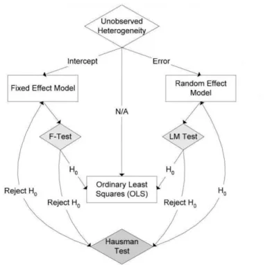
The following Figure 2 summarises the main steps required in a panel data analysis, in order to implement the most appropriate model for each situation and data specification.
14
13
Figure 2. Panel Data Modelling Process
Typically, an analysis conducted on panel data starts with a simple model, say the pooled OLS (POLS), and then investigates critically whether [un]observed heterogeneity might be taken into account and which model might be the most appropriate in this case.
The POLS assumes that the intercept and the slopes are constant across groups and time. Moreover, the individual effect does not exist in this first specification:
'CD = E + NCDO F + LCD P(2ℎ AC = 0
Due to its highest level of simplicity, the Pooled Ordinary Least Squares relies on a set of assumptions:
1. Linearity. The dependent variable is linearly composed from the independent variables and the error term
2. Exogeneity. The error is uncorrelated with the independent variables. In formulas, 4D LCD = 0 3% 4D NCDLCD = 0
3. Homoscedasticity. The error term has always the same variance, +3SD LCD = TIU
14
4D LCDLCV = 0 P(2ℎ 2 ≠ 1
5. Absence of multicollinearity. Regressors must be linearly independent or the regressor matrix must have full rank.
The violation of the second assumption, the one I will focus on, leads to a biased OLS estimator.
Further, if individual heterogeneity is present in the model (thus, AC ≠ 0), we will move to explore that impact through fixed effect (FE) model or random effect (RE) model. The former checks out possible variation in the intercepts (across time or group) and if the individual effect is correlated with the regressor(s). Mathematically, 'CD = E + AC + NCDO F + LCD. The latter identifies differences in error variance components which captures that heterogeneity, when the individual effect is not correlated with any regressor. In formulas, 'CD = E + NCDO F +
(AC+ LCD). Finally, all those models can be examined by conducting appropriate formal tests.
Here a list of those tests:
- F-test: It is used to explore the presence of FE and the improvements this model could introduce over the OLS specification. The null hypothesis proposes the non-correlation between that effect and the regressor(s), whereas the alternative hypothesis suggests that at least one parameter is different from zero. Hence, if H0 is rejected, the FE model is the most appropriate, otherwise the pooled OLS should be selected.
- Breusch-Pagan LM test: This test is conducted in order to assess the presence of RE and, hence, some heteroskedasticity in the model. The null hypothesis predicts that TYI = 0. If H0 is rejected, the RE model is the most appropriate, otherwise we should go for POLS.
15
regressors. The null hypothesis suggests the non-correlation between that effect and the regressor(s), whereas the alternative hypothesis claims the existence of that correlation. Hence, if H0 is rejected, the FE model is the most appropriate, otherwise the RE is the chosen one.
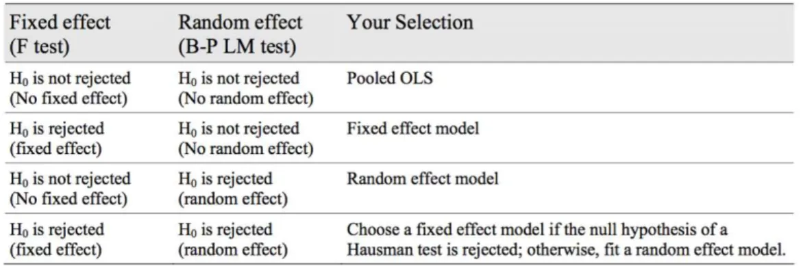
To conclude, Figure 3 provides an easily recap of the discussed tests and their outcomes.
Figure 3. Panel Data Formal Tests
Regression results and discussion
Before presenting the empirical results obtained, I will spend few words on the model selected following the steps just described in the previous section.
16
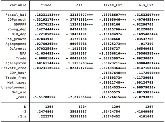
The results obtained by replicating the model of the Bruegel Working Paper are summarized in Figure 4, presenting both the fixed effect and the pooled OLS regressions. As shown, many variables are highly significant (p<0.001) and the majority is also in line with the theoretical predicted effect. For instance, in relation to the fiscal balance coefficient, this specification enhances the results obtained from the European Commission, which was negative and less significant. However, with regard to the population growth, our model improves the specification: In the Bruegel model the coefficient was both not significant and with the opposite site; conversely here, although still insignificant, the sign of that indicator is the same of the predicted one. Moreover, both NFA and openness to trade have an opposite sign, which is inconsistent with the theory and with Bruegel’s results. Those incongruences between our estimation and what obtained by Bruegel and Milesi-Ferretti could derive from the differences in the sample considered, both in terms of countries analysed and time-period covered. Therefore, our analysis suggests that an increase in the current account balance is caused by higher fiscal balance, slower growth differential, higher GDP per capita, smaller old-age dependency ratio, faster aging speed, larger oil rents, smaller NFA, lower trade openness and improved legal systems. The model explains around 22% of the variation in current account balances.
Next, as anticipated, I extended the model to include new current account determinants, in order to figure out if those additional control variables could help in better explaining the existing relation15. Those variables are:
• GDP per hour worked (measured in dollars at constant prices). It determines how efficiently input is aggregated with other factors and used in the production process.
15
17
Productivity improvements are likely to positively impact the current account balance; thus, the expected sign should be positive.
Data are collected from the OECD.Stat website.
• Freedom to trade internationally. It represents a proxy measure of the openness to trade that each country has.
Data are collected from the Economic Freedom Network.
• Net taxes on products (current dollars). Those are net indirect taxes on products, computed as the sum of product taxes less subsidies.
Data come from the World Development Indicators.
• Unemployment (as a percentage of the labor force). Commonly, the relationship between CA and this determinant is complicated. Some people believe that current account deficits are associated with higher level of unemployment. However, historical evidence reports a positive relationship since both macroeconomic elements are driven by cyclical economic factors.
Data are collected merging several databases, as the World Development Indicators, the IMF WEO and the OECD.Stat.
• Net bilateral aid (current dollars). These funds are bilateral flows that come from the Development Assistance Committee (DAC) donors and are represented as the net disbursements of Official Development Assistance (ODA) or official aid directly from the DAC16. In the short-run, a decreasing current account balance might be negatively affected by bilateral aids.
16
18
Data come from the World Development Indicators.
As reported in the right part of Figure 4, in the fixed effect specification only GDP per hour worked and unemployment indicators have a significative impact (at the 99.9% level) on the current account balance, while net taxes on product just at 99%.
Figure 4. Comparison Between Basic And Extended Model: Empirical Results
19
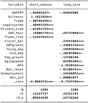
A step further can be done through a separation between short/medium-term and long-term variables, in order to analyse both current account cyclical and structural effects. The classification of those variables is provided by the EBA methodology17.
Figure 5. Current Account Structural VS Cyclical Effects: FE Estimation
Figure 5 above summarises the result obtained. For simplicity and in line with the previous part of the model, the results represented come from the FE specification.
Starting with the highly significant short/medium-term regressors, all of them maintain the same sign and also the coefficient is pretty close to the overall sample. Additionally, the freedom to trade internationally shows in this specification a higher level of significance, from 5% to 0.1%. Another improvement is reported by trade, which becomes significant (at 1%).
17
As already introduced in pag. 8.
Additionally, the nature of each variable is deeply analysed also in the following paper: “Structural and cyclical factors behind current-account balances”, Cheung, Furceri and Rusticelli (2010), OECDEconomics Department Working Paper. N. 775.
20
However, GDP per capita at PPP shows an opposite sign, if compared with the literature and with previous results.
With regard to the long-term variables, the first thing that should be highlighted is population growth: Even in this specification, the variable is not significant at all. Conversely, all other current account components preserve their sign and significance or even improve them (as happens for the old dependency ratio coefficient).
Finally, we should highlight the major contribution provided by the structural variables on the specification: Long-term determinants have a much higher impact in explaining the total variance, with an adjusted R-squared almost three times more than the one of cyclical variables.
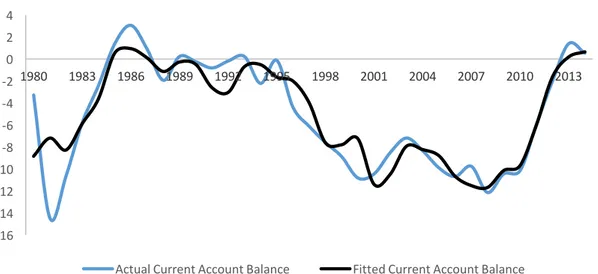
The last step further is done with a focus on the Portuguese case. In particular, the beta coefficients obtained from the extended model are used to compute the fitted current account values over the same horizon. The following Figure 6 represents the comparison between the actual current account values publicly recorded against the fitted values computed with this specification.
Figure 6. Portuguese Current Account Values: A Comparison Between Actual and Fitted Values -16
-14 -12 -10 -8 -6 -4 -2 0 2 4
1980 1983 1986 1989 1992 1995 1998 2001 2004 2007 2010 2013
Portuguese Current Account Balance: Actual VS Fitted Values
21
Focusing on the previous graph, we can assert that the fitted model predicts quite well the overall actual movements on the current account, especially in the last 30 years. However, the fitted model mitigates the impact of those CA variations, capturing them with a slightly lower severity. Beside this shortcoming, dependent variables have recently improved their predictive power in estimating the current account values: In effect, the obtained model can predict both upward and downward movements.
Conclusion
Between the end of the nineteenth century and the recent global crisis current account balances deteriorated several times, reaching the worst levels in 2008, after the negative values shown in both the oil crisis and the dot-com bubble. However, as highlighted by the European Commission, the actual scenario is widely heterogeneous: More developed and core countries show large and persistent surpluses whereas peripheral countries have large deficits.
In order to figure out various explanation for the changes in the current account levels and predict (im)balances future evolution, this paper used a panel econometric model to determine the components of current account balances and the existing link between them. That panel comprised a sample of 28 European countries from 1972 to 2014. Following previous literature, several variables were studied and those have confirmed that an increase in the current account balance is caused by higher fiscal balance, slower growth differential, higher GDP per capita, smaller old-age dependency ratio, faster aging speed, large oil rents, smaller NFA, lower trade openness and improved legal system.
22
current account balance. Further, a comparison between the two presented models suggests that the extended version provides a better explanation of the total variance (measured by the adjusted R-squared) than the basic model specification.
Moreover, the current account determinants were used to analyse both cyclical and structural effects through a separation between short/medium-term and long-term variables. As suggested in previous literature, this further analysis confirm that structural determinants provide the major contribution, explaining the total variance more than three times than the cyclical variables.
Lastly, the paper has investigated the Portuguese situation across the entire period (1972-2014), using the beta coefficients to obtain the fitted current account values and compare them with the actual current account values. Although the fitted model mitigates the impact of the current account determinants, capturing them with a slightly lower severity, the gap between those two values has a strong predictive power for future CA developments, mainly in recent times.
23
References
Brissimis, Sophocles. Hondroyiannis, George. Papazoglou, Christos. Tseveas, Nicholas
and Vasardani, Melina. 2010. “Current account determinants and external sustainability in periods of structural change”. European Central Bank. Working paper series N. 1243
Camacho, Máximo and Doménech, Rafael. 2010. “MICA-BBVA: A Factor Model of Economic and Financial Indicators for Short-term GDP Forecasting”. BBVA ResearchWorking Papers. N. 10/21
Cesaroni, Tatiana and De Santis, Roberta. 2015. “Current Account ‘Core-Periphery Dualism’ in the EMU”. CEPS Working Document. N. 406
Cheung, Calista. Furceri, Davide and Rusticelli Elena. 2010. “Structural and cyclical factors behind current-account balances”. OECD Economics Department Working Paper. N. 775
Darvas, Zsolt. 2015. “The grand divergence: Global and European current account surpluses”.
Bruegel Working Paper. 2015/08
European Commission. 2012. “Current account surpluses in the EU”. European Economy – Economic and Financial Affairs. European Commission. N. 9
European Commission. 2013. “The Macroeconomic Imbalance Procedure. Rationale, Process, Application: A Compendium”. DG ECFIN European Commission ***
European Commission. 2013. “Cyclical adjustment of current account balances”. DG ECFIN European Commission
European Commission. 2013. “Cyclical Vs. non-cyclical current account balances: a ‘joint estimation’ approach”. DG ECFIN European Commission ***
24
European Commission. 2013. “Updated Estimates of Cyclically-adjusted Current Account Balances November 2013 – Commission Autumn Forecast”. DG ECFIN European Commission ***
European Commission. 2014. “External rebalancing in the euro area: progress made and what remains to be done”. DG ECFIN European Commission ***
European Commission. 2015. “Report from the Commission to the European Parliament, the Council, the European Central Bank and the European Economic and Social Committee. Alert Mechanism Report 2016”. European Commission ***
European Commission. 2016. “Commission Staff Working Document. Country Report Portugal 2016. Including an in-Depth Review on the prevention and correction of macroeconomic imbalances”. European Commission ***
Fedora, Michael and Zorell, Nico. 2013. “Cyclically-adjusted current account balances for euro area countries”. DG EconomicsEuropean Central Bank. ***
Haltmaier, Jane. 2014. “Cyclically Adjusted Current Account Balances”. Board of Governors of the Federal Reserve System International Finance Discussion Papers. N. 1126
Herrmann, Sabine and Jochem, Axel. 2013. “Current account adjustment in EU countries: Does euro-area membership make a difference?”. Deutsche Bundesbank. Discussion paper 49/2013
IMF. 2013. “External Balance Assessment (EBA) Methodology: Technical Background”.
International Monetary Fund Research Department.
Kollmann, Robert. Ratto Marco. Roeger, Werner. Veld, Jan and Vogel, Lukas. 2014. “What drivers the German current account? And how does it affect other EU member states?”.
25
Salto, Matteo and Turrini, Alessandro. 2010. “Comparing alternative methodologies for real exchange rate assessment”. DG ECFIN, European Commission. Economic Papers 427/2010
Sastre, Teresa and Viani, Francesca. 2014. “Countries’ safety and competitiveness, and the estimation of current account misalignments”. Banco de España. Documentos de Trabajo N. 1041