This is an Open Access article distributed under the terms of the Creative Commons Attribution Non-Commercial License Received: 02 Mar., 2015
Accepted: 02 Mar., 2015
E-mail:
[email protected] (FS)
Abstract: In this paper the operator bias in the measurement process of arc efficiency in stationary direct current electrode negative gas tungsten arc welding is discussed. An experimental study involving 15 operators (enough to reach statistical significance) has been carried out with the purpose to estimate the arc efficiency from a specific procedure for calorimetric experiments. The measurement procedure consists of three manual operations which introduces operator bias in the measurement process. An additional relevant experiment highlights the consequences of estimating the arc voltage by measuring the potential between the terminals of the welding power source instead of measuring the potential between the electrode contact tube and the workpiece. The result of the study is a statistical evaluation of the operator bias influence on the estimate, showing that operator bias is negligible in the estimate considered here. On the contrary the consequences of neglecting welding leads voltage drop results in a significant under estimation of the arc efficiency.
Key-words: Arc efficiency; Gas tungsten arc welding; Direct current electrode negative; operator bias.
1. Introduction
The aim of this study is to evaluate the operator bias in the estimation of arc efficiency also known as process-, thermal- and heat transfer efficiency in stationary direct current electrode negative (DCEN) gas tungsten arc welding (GTAW). GTAW is one of the most widely used arc welding methods for welding stainless steels, thus representing an industrial process with significant economic importance. The arc efficiency in welding determines the weld bead formation, the formation of residual distortion and stress and also the metallurgical transformations. The metallurgy characteristics, consecutively, determine joint properties such as mechanical resistance, toughness and the degree of susceptibility to cold cracking etc. Hence, it is important to know how much of the
supplied energy that is transferred to the material being welded [1-3]. The arc efficiency
is also an important input to numerical heat-transfer models used for predictions and
understanding of the process [4].
A literature review by Stenbacka [5] covered the years between 1955 and 2011
shows that the arc efficiency values published for GTAW lie in a very wide range. The estimates were made from calorimetrical experiments and from calibrated simulation model results. Values between 0.36 and 0.90 are reported. A question arose about the
origins of this remarkable variance [5].
The evaluation method investigated is a common method based on calorimetric experiments. Estimations involving measurement procedures are always disposed to error in measurement and uncertainties. The measurement process errors include a number of factors such as tolerance limits of instruments, operator bias, errors arising from environmental conditions, or other sources. Furthermore, each measurement error
is considered to be a random variable characterized by a probability distribution [6]. As a
consequence the quantity in the context of the process together with the measurement process ought to be carefully explained in order to properly quantify a measurand by good statistical practice.
One important observation regarding arc efficiency in GTAW is that this parameter cannot be regarded as a universal constant. It is more or less dependent on the combination
Operator Bias in the Estimation of Arc Eiciency in Gas Tungsten Arc Welding
Fredrik Sikström1
although there are contradictions in statements between different references about the direction of this influence.
As an example [7] reported a decrease in arc efficiency with low weld travel speed and [8] reported an increase in
arc efficiency with low weld travel speed. Another parameter that significantly influences the arc efficiency is the welding power. Many authors have experimentally shown a decreased arc efficiency with increased weld current
and or increased arc length, see [9] for one example.
This study is limited to a stationary GTAW, DCEN process where most of the influencing parameters are kept constant in order to easier discriminate the operator bias in arc efficiency estimation.
2. Operator Bias and Environmental Factors Error
One of the major problems in conjunction with manual measurement is operator bias, which varies in degree according to the individual. Personal errors are due to, e.g. an inappropriate physical environment, procedural mistakes and lack of understanding of the process of measurement. Because of the possibility for human operators to acquire measurements from an individual perspective, it happens that two operators observing the same measurement will systematically produce different measured values. This operator bias has a random character due to inconsistencies in the human response. In addition to this error related to human behaviors significant measurement process errors might also result from variations in environmental conditions, such as temperature, humidity, vibration etc. In order to improve an estimate it is thus necessary to consider and evaluate these types of measurement process errors.
3. Arc Efficiency and Calorimetry
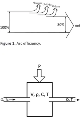
Arc efficiency defines the fraction of the arc energy transferred to the work piece. Commonly arc efficiency
is calculated as [10]:
(1)
where U and I are arc voltage and weld current respecively. qelectrode is the heat loss due to conducion in the weld electrode, q
arc is the heat radiated and convected from the arc column, qweld is the heat transferred to the base metal.
The fracion of heat transferred from the arc to the base metal is n, and m is the fracion of radiaion, convecion and possible evaporaion losses in the base metal. Figure 1 illustrates the assumed losses explained by Equaion 1.
The technique used in this study to estimate arc efficiency is water calorimetry, as principally is described
by e.g. [11, 12]. The method utilizes water cooling of the weld anode by a continuous water flow to remove heat
during welding. The water temperature difference between the inlet and outlet of the weld anode is recorded and the electrically induced heat input is related to the temperature rise of the cooling water. The arc efficiency is estimated by the following relation:
(2)
where t
weld is the total welding ime, Q is the volume rate of low of the cooling water, ñ and C are density 988 [kg/m
3]
and heat capacity of water 4180 [J/(kg·K)] respecively. Tin is the cooling water inlet temperature and Tout is the
outlet temperature. An approximaion is made in Equaion 2 by using the average esimate xi of each quanity
indicated by an over bar, and where ∆T = T
out – Tin. Figure 2 gives the principle of the calorimetry.
4. Experimental Procedure
A specially designed copper anode has been used as a calorimeter device together with a fixed weld torch, see Figure 3.
The power source used was a TIG Commander 400 AC/DC from Migatronic AB, and the weld torch was a
Wolfram Industrie GmbH and argon as a shielding gas was used. Table 1 provides the nominal welding parameters. The calorimeter inlet and outlet was instrumented with
thermocouples, type K, in order to acquire the history of this
temperature difference. The thermocouples were connected to an analogue input device from National Instrument, NI-9211 with a specified tolerance limit for temperature
measurements of ±1%. A flow meter, SF-800-3/8, from
SwissflowR with a specified tolerance limit of ±1%, was used to acquire the water flow rate. The weld current was measured with a Hall-effect transducer with a specified tolerance limit of ±1% and finally, the arc voltage was measured with an analogue voltage input device NI-9205. The voltage probe was connected to the electrode contact tube through a resistive voltage divider. The tolerance limit for the arc voltage measurement in this arrangement is estimated to be ±1%. All measured data were recorded with a sampling rate of 2 Hz and stored in a file for post analysis. The signal processing and recording was implemented in National Instrument’s LabVIEW software.
An additional relevant experiment consider the consequences of estimating the arc voltage by measuring the potential between the terminals of the weld power source instead of measuring the potential between the electrode contact tube and the workpiece. The result is a neglecting of the resistive power losses in the welding leads, including the electrode and ground cable and the resistive losses in the contact surfaces between connectors in the total electrical conductor. During welding with varying arc length and current an estimate of this loss was obtained. The estimate was based on 22 measurements where the voltage at the weld power terminals and the electrode contact tube was measured by a digital multimeter with an uncertainty of 1%. The corresponding weld current was measured by a digital clampmeter, also with an uncertainty of 1%.
4.1. Instructions for operators
The instructions for the operators were to use the nominal welding parameters provided in Table 1. In practice this involved manually adjustments of the arc length by using a set of gauge blocks, to manually adjust the shield gas flow rate reading a single flow tube rotameter, and finally to estimate the time when a steady state welding condition had been reached. When reaching the steady state welding condition the data acquisition system should then be turned on to acquire a sample of the signals consisted of at least 240 data during 120 seconds. Mean values of this sample was then used to estimate the arc efficiency according to the equation in the previous section. Fifteen individuals independently performed this estimate and reported their
Figure 1. Arc efficiency.
Figure 2. Principle of calorimetry.
Figure 3. Experimental setup with the calorimeter.
Table 1. Nominal welding parameters.
Parameter Value Unit
result. All persons are engineers or researchers and their report was given with the number of significant figures decided on their own.
5. Results
The resulting set of reported observations is a too small sample size (N=15) to conclude about normality
from a histogram, see Figure 4. Therefore a chi-square goodness-of-fit test [13] was performed. From this test it
was not possible to conclude about the set of observations if it was a normally distributed sample. However, it is reasonable to conclude from the central limit theorem that a sufficiently large number of observations, each with a well-defined mean and well-defined variance, will be approximately normally distributed. From these
considerations the median value of the reported data is used as an estimate of the arc efficiency, 0.80, and the
interquartile range, 0.01, is used to indicate variation.
This result could be compared with the estimate and the expanded uncertainty in the measurement in itself, assuming no operator bias. It is presumed that the measurement errors are statistically independent sources. The
combined uncertainty uc(η) is calculated as:
(3)
where X
i are the physical quaniies in the esimate of the arc eiciency η, xi are their esimate and are their
sensiivity coeicients. The expanded uncertainty is further calculated from uc(η) using a coverage factor k with
Equaion 3.
(4)
The resulting estimate of the arc efficiency calculated as in Equation 4 is, η(0.95) = 0.80 ± 0.03.
The reported uncertainty is an expanded uncertainty (Equation 4) calculated using a coverage factor of 2 which gives a level of confidence of approximately 95%. Table 2 gives an uncertainty budget including all sources of uncertainty in this combined measurement.
Figure 4. Reported observations of the arc efficiency. Mean value solid line and the interquartile range dotted lines.
Table 2. Uncertainty budget of the measurement.
Quantity, Xi Estimate, xi Standard uncertainty, u(xi) Sensitivity coefficient, Xi
∂η ∂
U 12.5 V 7.4·10–3 –6.2·10–2
I 75.0 A 0.86 –1.1·10–2
∆T 8.50 K 0.14 9.2·10–2
Q 21.0·10–6 m3/s 1.2·10–7 3.8·104
C 4180 J/(kg·K) 8.9·10–3 1.9·10–4
Since all the measurement uncertainties are specified as manufacturer tolerance limits they are treated as type B uncertainties with a rectangular probability distribution. This also applies to the parameter estimates of the thermophysical properties of water. Thus, the uncertainty
equation for each of them is where ±a are the
bounding limits.
A robust estimate of the welding leads resistivity was computed with a robust regression algorithm using iteratively reweighted least squares with a bisquare
weighting function [14-17]. Robust estimation was used
since the measurements were acquired during unknown experimental conditions where it is assumed that the variance in individual data was dependent on the data. Figure 5 shows the voltage drop over the welding leads
ΔU as a function of the weld current. The slope of thick
line is the estimate of the welding leads resistivity, R(0.95) = 0.01±0.001 Ω. The thin lines are the robust estimate of the standard deviation.
6. Discussion and Conclusion
For the cause of understanding the measurement process is relevant to evaluate the portion of the individual standard uncertainties in the combined uncertainty. Figure 6 shows a Pareto chart of the percent contribution to the
combined uncertainty uc(η). The influence of uncertainties
in the thermophysical properties of water is negligible justifying the use of constants in the calculation. The most prominent uncertainty is the temperature difference indicating that this measurement could benefit from using instruments with a narrower specification in the tolerance limit.
In the case when the estimate is based on measurements of the arc voltage on the weld power source terminals the resulting individual standard uncertainties in the combined uncertainty is shown in Figure 7.
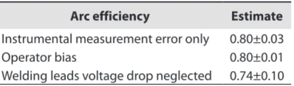
In this case the dominating source of uncertainty is obviously the arc voltage standard uncertainty. Table 3 gives the estimates of the arc efficiency considering the instrumental measurement error in one case, the operator bias in the other case and finally the case where the power loss in the welding leads is neglected.
It is clear that the operator bias is of minor importance. The underestimation of the arc efficiency due to power losses in the welding leads can be an explanation to some
of the published low values highlighted in [5]. Furthermore
it is reasonable to assume that other factors than the scalar electrical power influences the arc efficiency. For instance, the arc length and weld current have a significant influence. With increasing current and arc length, both
Figure 5. Voltage drop in welding leads.
Figure 6. Relative contribution to uc(η) during nominal measurement conditions.
Figure 7. Relative contribution to uc(η) reflecting a systematic error in the arc voltage measurement.
Table 3. Estimates of arc efficiency.
Arc efficiency Estimate
the mean temperature [18] and the radiation source strength in the arc column are rising which in turn causes
higher radiation losses. The arc shape and heat source distribution is affected by variations in all of the nominal parameters given in Table 1. And even by other parameters like features in the electrode tip geometry as well as shielding gas composition, the material being welded and the weld travel speed etc. The arc efficiency is clearly affected by the arc geometry and its heat source distribution. This means in practice that an accurate arc efficiency estimate only can be made with knowledge of all these various aspects.
Acknowledgements
This research work is supported in part by grants from the KK-foundation, which is gratefully acknowledged.
The author would like to thank Nils Stenbacka, University West, for his valuable comments on the content, and
also Kjell Hurtig, University West, for his practical contributions in the laboratory. Thanks is also given to Petter Hagqvist, Anders Appelgren, Patrik Broberg, Leif Karlsson, Hans Dahlin, Hans Åström, Mattias Ottosson, Morgan
Nilsson, Stefan Björklund, Mohit Gupta, Lyphout, Christophe, Jeroen De Backer, Ulf Hulling and Almir Heralic who acted as independent human operators during the measurement process. All are colleagues at University West.
References
[1] Lindgren L-E. Computational welding mechanics: thermomechanical and microstructural simulations. Cambridge: Woodhead Publising; 2007. 231 p. (Woodhead Publishing Series in Welding and Other Joining Technologies).
[2] Radaj D. Heat effects of welding: temperature field, residual stress, distortion. Berlin: Heidelberg; New York: Springer; 1992. 348 p. http://dx.doi.org/10.1007/978-3-642-48640-1. [3] Lancaster JF. The physics of welding. 2nd ed. Oxford: International
Institute of Welding; New York: Pergamon; 1986. 340.
[4] Mishra S, DebRoy T. A heat-transfer and fluid-flow-based model to obtain a specific weld geometry using various combinations of welding variables. Journal of Applied Physics. 2005;98(4):044902.
http://dx.doi.org/10.1063/1.2001153.
[5] Stenbacka N. On arc efficiency in gas tungsten arc welding. Soldagem & Inspeção. 2013;18(4):380-390. http://dx.doi.
org/10.1590/S0104-92242013000400010.
[6] Bureau International des Poids et Mesures – BIPM. GUM: Guide to the Expression of Uncertainty in Measurement. Geneva: International Organization for Standardization; 2008.
[7] Fuerschbach PW, Knorovsky G. A study of melting efficiency
in plasma arc and gas tungsten arc welding. Welding Journal. 1991;70(11):287s-297s.
[8] Dutta P, Joshi Y, Franche C. Determination of gas tungsten arc welding efficiencies. Experimental Thermal and Fluid Science. 1994;9(1):80-89. http://dx.doi.org/10.1016/0894-1777(94)90011-6. [9] Åström H. Arc efficiency for Gas Tungsten Arc Welding – GTAW.
In JOM-17 International Conference; 2013 May 5-8; Helsingör,
Denmark. Helsingör: Institute for the Joining of Materials; 2013.
[10] Nguyen NT. Thermal analysis of welds developments in heat transfer. Southampton: WIT; 2004. 334 p.
[11] Lu MJ, Kou S. Power inputs in gas metal arc welding of aluminum
- Part 1. Welding Journal. 1989;68(9):382s-388s.
[12] Lu MJ, Kou S. Power inputs in gas metal arc welding of aluminum
- Part 2. Welding Journal. 1989;68(11):452s-456s.
[13] Thode HC. Testing for normality. New York: Marcel Dekker; 2002. http://dx.doi.org/10.1201/9780203910894.
[14] DuMouchel W, O’Brien F. Integrating a robust option into a multiple regression computing environment. In: Malone L, Berk
K, editors. Computer Science and Statistics: Proceedings of the
21st Symposium on the Interface; 1989 April 9-12; Alexandria, USA. Alexandria: American Statistical Association; 1989. p. 297-301.
[15] Street JO, Carroll RJRJ, Ruppert D. A note on computing robust regression estimates via iteratively reweighted least squares. The American Statistician. 1988;42(2):152-154.
[16] Holland PW, Welsch RE. Robust regression using iteratively reweighted least-squares. Communications in Statistics. Theory and Methods. 1977;6(9):813-827. http://dx.doi.
org/10.1080/03610927708827533.
[17] Huber PJ. Robust statistics. New York: John Wiley and Sons; 1981. http://dx.doi.org/10.1002/0471725250.