Simulation of Geomagnetic Reversals Through
Magnetic Critical Models
V. H. A. Dias, J. O. O. Franco, and A. R. R. Papa Observat´orio Nacional, Rua General Jos´e Cristino 77, S˜ao Crist´ov˜ao, Rio de Janeiro, 20921-400 RJ, BRAZIL
and
Universidade do Estado do Rio de Janeiro, Rua S˜ao Francisco Xavier 524, Maracan˜a, Rio de Janeiro, 20550-900 RJ, BRAZIL
Received on 29 September, 2007
We use numerical simulations of a well-known phase-transition model to study reversals of the geomagnetic field. Each ring current in the geodynamo was supposed to behave as a magnetic spin while the magnetization of the model was supposed to be proportional to the Earth’s magnetic dipole. We have performed a size-dependence study of the calculated quantities. Power laws were obtained for the distribution of times between reversals. Some of our results are closer to actual ones than the corresponding to previous simulations. For the largest systems that we have simulated the exponent of the power law tends towards values very near -1.5, generally accepted as the right value for this phenomenon. Some possible trends for future works are advanced.
Keywords: Ising model; Reversals; Computer simulation
I. INTRODUCTION
During the last decades many research efforts of statistical physicists have been devoted to the study of the earthquake problem [1]. However, it is far from being the unique geo-physical subject where statistical physics could bring some light. Let us mention the problems of magnetic storms [2,3] and geomagnetic reversals [4]. We will focus our attention on geomagnetic reversals.
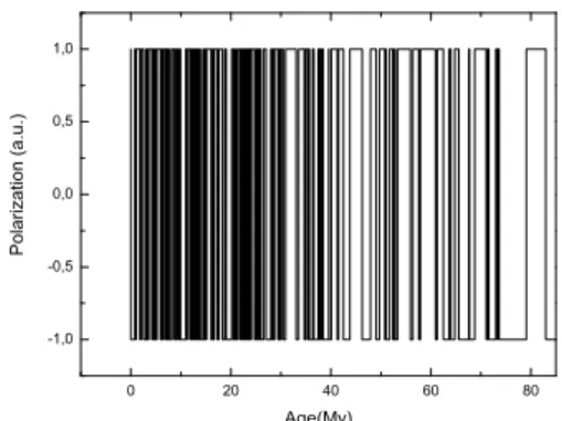
The field produced at the interior of the planet has its main source in a complex system of internal currents that eventu-ally produce geomagnetic reversals. They are periods during which the Earth’s magnetic field swaps hemispheres. Many of them have been documented. Periods between geomagnetic reversals present power law distribution functions, which can be the signature of some critical system as the mechanism of their source [5]. There are other mechanisms capable of pro-ducing power laws (for example, superposition of some dis-tributions [1], self-organized criticality [6] and non-extensive versions of statistical mechanics [7]) but we will not extend on them upon here. In Fig. 1 we present the sequence of geomag-netic reversals from 80 million years (My) to our days. The data was obtained from the most recent and complete record that we have found [8,9]. Fig. 2 presents the distribution of periods between reversals, it follows a power law,
f(t) =ctd (1)
where f(t)is the frequency distribution of periods between consecutive reversals,cis a proportionality constant andd is the exponent of the power-law and the slope of the graph in log-log plots. For the present case we have approximately -1.5 as slope value.
The magnetic field needs a finite time to change its direction (the time between the moment at which the dipolar component is no more the main one and the moment at
0 20 40 60 80
-1,0 -0,5 0,0 0,5 1,0
P
o
l
a
r
i
za
t
i
o
n
(
a
.
u
.
)
Age(My)
FIG. 1: Representation of geomagnetic reversals from around 80 My ago to our days. We arbitrarily have assumed -1 as the current polar-ization. We have not plotted the period from 80 My to 165 My (for which also a record exists) for the sake of clarity. There was a period with no reversals from 80 to 120 My (the beginning appears in the plot). The period from 120 My to 165 My was very similar to the period from 0 to 40 My (in number of reversals and in the average duration of reversals). The data was obtained from Cande and Kent [8,9].
which it is again the main one but building up in the opposite direction). This time is in the average around 5000 years. It is small if compared to the smallest interval between reversals already detected ( 10,000 years) and to the average interval between reversals. There are clustered periods of high activity from 40 My ago to our days and during the period 165-120 My (not shown), a period of low activity between 80 and 40 My ago and a period of almost null activity from 120 to 80 My.
0,1 1 1
10 100
F
r
e
q
u
e
n
cy
Time (My)
FIG. 2: Frequency distribution of periods between reversals from 80 My to our days. The slope of the solid line is around -1.5. The data was obtained from Cande and Kent [8,9].
seems to increase with geological time. Unfortunately, the reversal series is unique and relatively small, there is no other similar record (for earthquakes, for example, exists a record for each fault, and from the Moon obtained during the Apollo program).
-20 -10 0 10 20
0 5 10 15 20
N
u
m
b
e
r
o
f
sa
m
p
l
e
s
VDM (10 22
Am 2
)
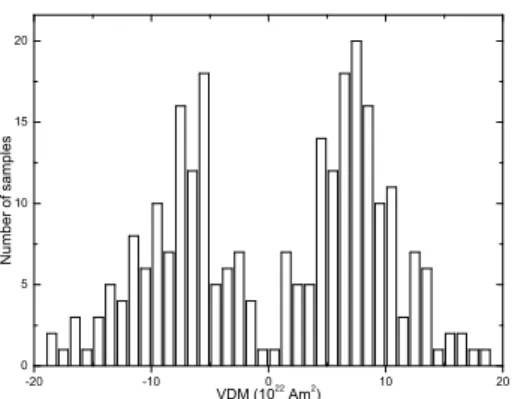
FIG. 3: Distribution of virtual dipole moment (VDM) values for sam-ples not older than 10 My. Negative values of VDM correspond to reverse polarization and are represented by 119 samples. Positive values of VDM represent normal polarization and are represented by 142 samples. The data was obtained from Kono and Tanaka [10].
Contrary to the record of reversals (known from 160 My up to nowadays) the record of magnetic field intensities exists just for around 10 My [10]. Fig. 3 shows the distribution of Earth’s dipole values for the last 10 My. The distribution of dipole values for actual reversals (Fig. 3) follows a func-tion between a bi-normal and a bi-log-normal distribufunc-tion. However, the number of experimental points is also small and there will certainly be changes in these facts when new measurements become available.
Geomagnetic reversals have called a great attention since
their discovery and this interest remains nowadays. Works devoted to the study of the time distribution of geomagnetic reversals include, among many others, statistical studies on reversals distributions and correlations [5,11-13], modelling of the problem [14-16] and experimental studies [8,9,17-19]. Gaffin [11] pointed out that long-term trends and non-stationary characteristics of the record could hamper a formal detection of chaos in geomagnetic reversal record. It is our opinion that actually it is very difficult to detect in a consistent manner that geomagnetic reversals present any systematic characteristic at all, without mattering which this characteristic could be (including chaos). Its nature remains an open question.
In this work we use the 2D Ising model nearTcto mimic the
Earth’s magnetic field and its reversals. Ising systems have already been used to simulate reversals of the Earth magnetic field [16]. Our work differs from it in that while they used the Q2R automata we have used a regular Metropolis updating algorithm around the critical temperature. Some of our results also differ essentially from them and are closer to actual ones. The study of geomagnetic reversals can contribute to the comprehension of important processes in Earth’s evolution. This includes from the internal dynamics of the planet to processes involving the evolution of living organisms. The Earth is continuously bombarded by charged particles mainly born at the Sun. Large fluxes of those particles are incompat-ible with life. Fortunately, only a tiny fraction of them hits the Earth’s surface. The most part is deviated by the geomag-netic field. However, during reversals the field intensity de-creases drastically which means a more intense bombarding. The ”magnetic shield” is reduced. Those increases in the flux of particles could have interfered in life cycles of the planet.
II. THE MODEL
Simulation of the core by three-dimensional magnetohy-drodynamic equations is an extremely difficult task [14,15]. To diminish the number of degrees of freedom an alternative way is to use N coupled disk dynamos models [20]. Follow-ing Seki and Ito [16] we further simplified the last one by associating spins to currents.
The Ising model is some kind of paradigm among magnetic models for condensed matter because it is the simplest one that presents a phase transition at temperatures different from zero (inD>1, where D is the dimension). But Ising models have found applications in areas away from solid-state physics, for example, in immunology [21], stock market theory [22] and earthquake dynamics [23], among many others. In this work we use the 2D Ising model to simulate the Earth’s dynamo, particularly the reversals of the Earth’s magnetic field.
fact that the dipole suffers reversals, in a similar way to the Ising model near the critical temperature. From the practical point of view the motivation comes from the possibility of generate good synthetic data with simple models to diminish the problem of limited availability of experimental data.
In absence of external field the HamiltonianHfor the Ising model is:
H=−J
∑
i,j
sisj (2)
where the sum runs over all neighbor pairs,siandsjare spins
andJis the interaction constant between spins. The critical temperature of the Ising system for 2D isTc= 2.269 in units of J/kB, wherekBis the Boltzmann constant. By definition, each
spinsican assume only two values or orientations: 1 and -1.
It is worth to mention that the Ising model was introduced by Wilhelm Lenz in 1920 and exactly solved for one dimension by his student Ernest Ising, in 1925, and in two dimensions by Lars Onsager, in 1944. It was shown that for 2D there is a phase transition.
In our model we assume, following Seki and Ito [16], that each spin represents a current ring in the Earth’s dynamo (i.e., that turbulent eddies behave as magnetic spins).
The magnetizationMfor the model is defined as:
M=∑
N i=1si
N (3)
where the sum runs over all the spins andNis the total number of spins. It can take values between -1 and 1. It is assumed in our model that the magnetization represents the geomagnetic dipole.
Now we call the attention to the fact that the magnetic mo-ment of eddies are of vectorial nature (they are not restricted to values+1 or−1) and, in principle, they exist in a broad range of sizes (limited uniquely by the core size). Later will be clear that in ferro-magnetic-like simulations domains of spins with the same orientation can be considered to represent larger ed-dies while, in anti-ferrimagnetic-like simulations this distinc-tion have to be imposed by us. On the other hand, the idea of neighbor eddies is customarily used in the study of such phe-nomena (we refer the interested reader to the book by Merril et al. [4]).
Many efforts have been made to enlarge the size of simu-lated Ising models when trying to represent systems of phys-ical or biologphys-ical nature [24]. The reason is simple: the numbers of elements in condensed matter physics and bio-logical systems are usually huge, around 1023 and 1014, re-spectively. Physical models for the Earth’s magnetic field are mostly based in a small number of adequately connected dy-namos. Using small 2D Ising systems to simulate their inter-action and behavior must sound a natural choice. We have performed simulations on 2D square Ising systems at temper-atures nearTcand studied some of the relevant characteristics
of the distribution in time of magnetization reversals (transi-tions between states of positive and negative magnetization). We have applied periodic boundary conditions [25]. At the
same time we have studied the size dependence of distribu-tions. We have usedLxLsystems whereL= 5, 10, 20, 30, 40 and 50.
We believe that the Ising model nearTc could be a good
model for reversals of the Earth’s magnetic field because of the critical character present in the Ising model and suggested by figures 2 and 3 (see below). The resulting magnetic field of the Earth is the superposition of several components (dipolar, quadripolar, and so on). When we simulate reversals through 2D Ising systems we are mainly focusing on the dipolar mo-ment (which is the main component the most part of the time). In this way, we are able to mimic the essentially 3D Earth by a 2D Ising system. The rotation of the Earth imposes a preferen-tial direction to the possible orientations of magnetic moments associate to eddies. From both dynamo-like and convection-like approaches, the structures in the core are of tubular type with symmetry axes parallel to the rotation axis of the Earth. At the same time, those structures traverse the core from the bottom to the top (top meaning the ”superior” hemisphere and bottom meaning ”inferior” hemisphere). This facts support the simulation of a 3D system by a 2D one. The magnetic field, however, never reaches the value ”zero”. It diminishes to values very near zero in other directions than the north south one.
III. RESULTS AND DISCUSSION A. Ito and Seki simulations
1 10 100 1000 10000
1 10 100 1000
F
r
e
q
u
e
n
cy
(
a
b
o
ve
a
g
ive
n
va
lu
e
)
Time (Q2R steps)
FIG. 4: Frequency distribution inter-reversal periods (Ito and Seki model). The solid line slope is -0.5 which means -1.5 for a normal (not above-a-given-value) histogram, as in Fig. 2.
How--1,0 -0,5 0,0 0,5 1,0 0,0
0,2 0,4 0,6 0,8 1,0
N
o
r
m
a
l
i
ze
d
f
r
e
q
u
e
n
cy
Magnetization
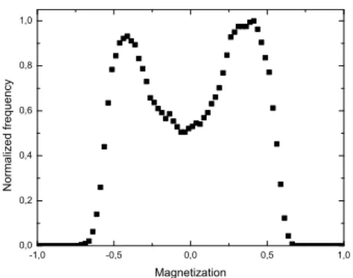
FIG. 5: Frequency distribution of magnetization values (Ito and Seki model). Note that the central valley is around 50 percent of the peaks highs while for actual measurements (Fig. 3) it is less than 10 percent.
0 200 400 600 800 1000
-1,0 -0,5 0,0 0,5 1,0
0 2000 4000 6000 8000 10000
-1,0 -0,5 0,0 0,5 1,0
M
a
g
n
e
ti
z
a
t
io
n
Tim e (MCS/s)
b
M
a
g
n
e
t
i
z
a
t
io
n
Time (MCS/s)
a
FIG. 6: Time dependence of the magnetization for temperatures slightly belowTc(T= 2.26). a) A sample of 1000 MCS/s pertaining
to a long run. b) A longer sample (up to 10000 MCS/s). Both cases correspond to a 5x5 system size.
ever, we note that the relative high of the valley is much more higher than for actual measurements (Fig. 3).
B. Ferromagnetic Metropolis simulations
Next, we have simulated the Ito and Seki model using in-stead of the Q2R a Metropolis updating algorithm. In Fig. 6 we show some typical time dependence of magnetization for temperatures slightly below Tc. They qualitatively resemble
the results presented in Figs. 3 and 5 of reference [16]. How-ever, they are quantitatively different from them (see below). Fig. 7 shows the result of eliminating all the fluctuations in Fig. 6b. We have only marked the jumps through the value zero and assigned a value 1 to all the positive values and -1 for the negative ones. Note the pictorial and qualitative similari-ties between Figs. 1 and 7. In particular, note that Fig. 7 also presents clustered periods of greater activity (between 7000 and 10000 MCS/s) and of lower activity (between 6000 and 7000 MCS/s and around 1000 MCS/s, for example).
0 2000 4000 6000 8000 10000
-1,0 -0,5 0,0 0,5 1,0
P
o
l
a
r
i
za
t
i
o
n
Time (MCS/s)
FIG. 7: A binary version of the dependence in Fig. 2b. It was as-signed a value 1 to all valuesM>0 and a value of -1 for all values M<0. Note the similarity with Fig. 1 where actual reversals are presented.
Figure 8 shows the distribution of intervals between consec-utive reversals (T=2.26) for different system sizes. The bold straight line is a guide for the eye in all cases. The distrib-ution follows a power law. However its apparition presents a size dependence. For larger periods the distribution fol-lows an exponential. The exponential dependence can eas-ily be confirmed by representing the data in a semi-log graph (not shown). For 5x5 systems the exponential occupies almost all the histogram interval (Fig. 8a) while for systems of size 50x50 it is almost inexistent (Fig. 8c). We have not found the initial power law dependence in the literature but in our sim-ulations and in the work by Seki and Ito [16]. This is a quite remarkable fact given that the Ising model has been analyti-cally and computationally (very extensively) explored during many years. In Fig. 9 it is shown the size dependence of the power-law exponent for a fixed temperatureT = 2.26 (very nearTc). Data is satisfactorily fitted by an exponential
func-tion. The results for the slope value range from -2.0 (for 5x5 systems) to -1.55 (for 50x50 systems). As can be seen, the larger the system the closer to the most accepted value (-1.5) for the slope on actual reversals distribution [4].
1 10 100 1
10 100 1000
1 10 100
1 10 100
F
r
e
q
u
e
n
c
y
Tim e (MCS/s)
c
1 10 100 1000
1 10 100 1000
F
r
e
q
u
e
n
c
y
Tim e (MCS/s)
b
F
r
e
q
u
e
n
c
y
T im e (MCS/s)
a
FIG. 8: Distribution of periods between consecutive reversals for our model. The system sizes are 5x5, 10x10 and 50x50 for a), b) and c), respectively. In all cases the bold straight line is a guide for the eye. Slopes values are a) -2.0, b) -1.87 and c) -1.55. Runs were done at a fixedT=2.26.
0 500 1000 1500 2000 2500
-2,0 -1,9 -1,8 -1,7 -1,6 -1,5
d
System size
FIG. 9: Size dependence for the slope of the distribution of periods between consecutive reversals in our model. The bold curve is an exponential fit to data. It has the formy=y0+A.exp(−x/t), where
y0=−1.559±0.014,A=−0.457±0.023 andt=326±49.
-1,0 -0,5 0,0 0,5 1,0
0,0 0,2 0,4 0,6 0,8 1,0
R
e
l
a
t
ive
f
r
e
q
u
e
n
cy
Magnetization
FIG. 10: Distributions of magnetization values. For 5x5 systems (squares) the maxima appear at the extremes. For larger systems, and in particular for 50x50 systems (circles), maxima appear at values of magnetization|M| 6=1. The valley value is around 10 percent of the peaks values, closer to actual measurements than Ito and Seki simulations.
2,18 2,20 2,22 2,24 2,26 2,28 2,30 2,32 2,34 2,36 2,38
0,00 0,01 0,02 0,03 0,04 0,05
(
N
u
m
b
e
r
o
f
r
e
ve
r
sa
l
s
i
n
1
0
7
M
C
s/
s)
-1
Temperature
FIG. 11: Temperature dependence of the mean time interval between consecutive reversals. For temperatures below 2.18 there were no reversals (for simulations up to 106MCS/s).
2,25 2,30 2,35 2,40 2,45 2,50 2,55 2,60
-2,6 -2,4 -2,2 -2,0 -1,8 -1,6 -1,4
d
Temperature
T C
0 10 20 30 40 50 100
1000
M
e
a
n
i
n
t
e
r
va
l
b
e
t
w
e
e
n
r
e
ve
r
sa
l
s
(
M
C
s/
s)
L
FIG. 13: Size dependence of the mean time interval between con-secutive reversals. The same temperatureT = 2.26 was used in all cases. The straight bold line is an exponential fit∼exp(const.L)(for systemsLxL).
FIG. 14: Schematic representation of the a) mechanical; and b) mag-netic; interaction between idealized neighbor eddies. In a) we present a view from above (perpendicular to the plane containing eddies). In b) we present a side view; the central dipole interacs favorably with the left one.
there are not counterparts, for larger systems, a fluctuation to an absolute value near 1 in a part of the system will be accompanied almost always by a value far from those values in other pieces of the system. Like in [16] the distributions follow very roughly a bi-normal function. However, in a previous work [26] on block distribution functions for the Ising model in 2D, 3D and 4D the test was done formally and it was clear that they do not obey gaussians distributions. In this particular our simulations are superior to those by Seki and Ito [16]. We have reproduced their simulations and obtained that, while in our simulations (and in actual reversals) the distribution highs for zero magnetization is around 0.1 of the maximum, for Q2R simulations it is around 50 percent. This difference is probably associated to the
-0,02 -0,01 0,00 0,01 0,02 0,03 0,04
0 5000 10000 15000 20000 25000 30000
0 2 4 6810121416
1 10 100 1000 10000 100000
Fr
e
q
u
e
n
c
y
Time between reversal (MCS/s)
F
r
e
q
u
e
n
cy
Magnetization
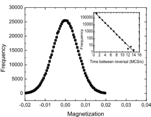
FIG. 15: Frequency distribution of magnetization values (Ising, an-tiferromagnetic, Metropolis). The magnetization is not a good order parameter, its distribution around zero is a gaussian. The inset shows the distribution of periods between reversals. Note that it is presented in a semi-log plot, so the line is not a power-law but an exponential.
10 100 1000
1 10 100 1000
F
r
e
q
u
e
n
cy
(
a
b
o
ve
a
g
i
ve
n
va
l
u
e
)
Time between reversals (MCs/s)
FIG. 16: Frequency distribution of inter-reversal periods (Ising, an-tiferrimagnetic, Metropolis). The solid line has a slope value around -0.5.
-2000 -1000 0 1000 2000
0,0 0,2 0,4 0,6 0,8 1,0
F
r
e
q
u
e
n
cy
(
n
o
r
m
a
l
i
ze
d
)
Magnetization
non-ergodic character of Q2R simulations.
Figure 11 shows the dependence of the average duration of time intervals between consecutive reversals on temperature (always for temperatures near the critical point). These results can help us to understand the way in which external factors affect the reversal regime. For more intense perturbations (high temperatures) the reversals are more frequent. For less intense perturbations (low temperatures) there is a lower number of reversals for time unit.
In our simulations the temperature plays the role of a tuning parameter. For temperatures well aboveTcwe observe
only small fluctuations aroundM = 0, for temperatures well belowTcwe observe a state of constant magnetization values
1 or -1 with seldom flips to -1 or 1 values, respectively. We have studied the dependence of the power-law slope on temperature for temperatures T around Tc (Fig. 12). Note
that for temperatures near Tc or above the slope remains
almost constant and in a narrow interval (from -1.75 to -1.55). Another point to be highlighted in Figure 12 is that for temperatures above and belowTc the physics under
magnetization reversals are very different. For temperatures below Tc it is essentially a tunnelling through an energy
barrier while for temperatures aboveTcit is well represented
by random walks returns to the origin. However, the slope of the inter-reversal interval distribution change in a very gradually manner (at least up to the temperatures that we have simulated).
Figure 13 presents the mean interval between consecutive reversals as a function of the system size. This dependence gives some qualitative insight on which is the volume of Earth’s interior that effectively carries the currents that produce the magnetic field (but equally, it could be associated to the number of eddie currents effectively producing the magnetic field). For larger systems reversals are less fre-quent than for small systems. As expected [27] the data in Fig. 13 can be satisfactorily fitted by an exponential function
exp(const.L)forLxLsystem sizes.
Despite of the dynamical character of reversals mentioned at the introductory section, there are some pieces of our simulations very similar to the actual sequence of reversals. That is the case in Fig. 7, for example, between Montecarlo steps of numbers around 1000. Probably, some historical ingredient, (i.e., a non-equilibrium approach) could be taken in future attempts to describe the phenomenon. Such an ingredient lacks in our work. Simulations with varying temperature or system size are two of the possibilities opened by the present approach.
C. Anti-ferromagnetic Metropolis simulations
Following Ito and Seki we have initially used a ferromag-netic version of the Ising model to simulate the geodynamo.
However, an anti-ferromagnetic type of interaction seems to better represent actual eddies interactions. The mag-netic moment of neighbor eddies is more favorable to an anti-ferromagnetic-like arrange both mechanically and mag-netically as illustrated in Fig. 14. We have simulated 50x50 2D Ising anti-ferromagnetic systems. (the same Hamiltonian than in Equation (2) except for the minus sign). Unfortu-nately, the magnetization is not a good order parameter for antiferromagnetic systems and the result for the distribution of magnetization values around zero give a Gaussian as can be seen in Fig. 15. The distribution for periods between reversals is of exponential type (see the inset of Fig. 15).
D. Metropolis Anti-ferrimagnetic simulations
An improvement in the model is the introduction of different sizes for spins. We have done this by simulating an anti-ferrimagnetic system (the same Hamiltonian than in Equation (2) except for the minus sign and for the fact that neighbor spins have no more the same value) where it was supposed that the spin size in a sublattice is twice the size of the spin in the other sublattice (raising the critical temperature to the double of lattices where all the spins have the same absolute value).
We present in Fig. 16 the distribution of periods between reversals for 50x50 anti-ferrimagnetic systems. The value near -0.5 for the slope remains (as in Ito and Seki and ferro-magnetic models). Our field reversal exponent is closely related to the global persistent exponent [28]. The last one is calculated from simultaneously evolving many systems until the magnetization first change sign and keeping track of the fraction p(t)of surviving systems (systems that have not suffered a reversal up to timet). Our exponent is calculated from following a single system and recording time intervals between consecutive reversals. It is our believe that they describe essentially the same phenomena.
In Figure 17 the distribution of magnetization values for the same system is shown. Once more two peaks are present as well as a valley with less than 10 percent of peaks’ highs. Comparison of results in figures like Fig. 17 and results in Fig. 3 must be done carefully. Note that the results in Fig. 3 are unbounded (the only possible bound could be the dipole value for the case in which the whole core rotates as a single unit). The usual values seem to be far from this bound. Our results, on the other hand, have a bound±1 imposed by the model. This factor give one possible direction for future works.
IV. CONCLUSIONS
tem-perature, the slope of the distribution of times between rever-sals has a smooth dependence on temperature. This fact will eventually need a deeper study. There is a dependence of the mean interval between reversals in both temperature and sys-tem size. However, as shown, all the studied properties reach stationary values for relatively small systems, which permits to use the temperature as the unique free parameter. There are two points to be highlighted: first, that as in our simulations the actual distribution of intensities has a deep valley (ampli-tude approximately 0.1 of the maximum) for magnetization values near zero; and second, that our simulations reproduce the power law dependence of actual reversals (with a slope value very near the actual one). In this sense our simulations (Metropolis) are superior when compared to Q2R simulations.
The necessity of more detailed models including, for example, the fact that there is a continuous scale of eddies is apparent. Some works are currently running along these lines and will be published elsewhere.
Acknowledgments
The authors sincerely acknowledge partial financial sup-ports from FAPERJ (Rio de Janeiro Founding Agency) and CNPq (Brazilian Founding Agency). We are indebted to an anonymous reviewer whose criticisms and comments have greatly helped in the final presentation of the work.
[1] D. Sornette, Critical Phenomena in Natural Sciences, (Springer, Berlin, 2004).
[2] A. R. R. Papa, L. M. Barreto, and N. A. B. Seixas, J. Atm. Sol. Terr. Phys.,68, 930 (2006).
[3] Magnetic storms are periods that last from one to three days during which the field suffers rapid variations. (2004), however, they seriously affect many human activities. They are mainly caused by phenomena in the Sun that affect the Earth’s at-mosphere.
[4] R. T. Merrill, M. W. McElhinny, and P. L. McFadden,The mag-netic field of the Earth; Paleomagnetism, the Core, and the Deep Mantle, (Academic Press, 3rd Ed., San Diego, 1998). [5] A. R. T. Jonkers, Phys. Earth Planet. Int.,135, 253 (2003). [6] P. Bak, C. Tang, and K. Wiesenfeld, Phys. Rev. Lett.59, 381
(1987).
[7] M. Gell-mann and C. Tsallis,Nonextensive entropy: interdisci-plinary applications, (Oxford University Press, Oxford, 2004). [8] S. C. Cande and D. V. Kent, J. Geophys. Res.97, 13917 (1992). [9] S. C. Cande and D. V. Kent, J. Geophys. Res.100, 6093 (1995). [10] M. Kono and H. Tanaka,In: The Earth’s Central Part: Its struc-ture and Dynamics, (T. Yukutabe, Ed. Terrapub, Tokyo, 1995). [11] S. Gaffin, Phys. Earth Planet. Int.57, 284 (1989).
[12] C. Constable and C. Johnson, Phys. Earth Planet. Int.153, 61 (2005).
[13] M. Cortini and C. Barton, J. Geophys. Res.99, 18021 (1994).
[14] P. D. Mininni, A. G. Pouquet, and D. C. Montgomery, Phys. Rev. Lett.97, 244503 (2006).
[15] P. D. Mininni and D. C. Montgomery, Phys. Fluids18, 116602 (2006).
[16] M. Seki and K. Ito, J. Geomag. Geoelectr.45, 79 (1993). [17] R. Zhu, K. A. Hoffman, Y. Pan, R. Shi, and D. Li, Phys. Earth
Planet. Int.136, 187 (2003).
[18] B. M. Clement, Nature428, 637 (2004).
[19] J.-P. Valet, L. Meynadier, and Y. Guyodo, Nature, 435, 802 (2005).
[20] M. Shimizu and Y. Honkura, J. Geomag. Geoelectr. 37, 455 (1985).
[21] D. Stauffer, Int. J. Mod. Phys. C5, 513 (1993).
[22] L. R. da Silva and D. Stauffer, Physica A,294, 235 (2001). [23] A. Jimenez, K. F. Tiampo, and A. M. Posadas, Nonlin.
Processes Geophys.14, 5 (2007). [24] D. Stauffer, Physica A244, 344 (1997).
[25] A. R. R. Papa, Int. J. Mod. Phys. C9, 881 (1998). [26] K. Binder , Z. Phys. B - Cond. Mat.43, 119 (1981).
[27] H. Meyer-Ortmanns and T. Trappenberg, J. Stat. Phys.58, 185 (1990).