Scalar Meson
σ
Phase Motion at
D
+
→
π
−
π
+
π
+
Decay
Ignacio Bediaga
Centro Brasileiro de Pesquisas F´ısicas-CBPF Rua Xavier Sigaud 150, 22290-180 Rio de Janeiro, Brazil
(Representing the Fermilab E791 collaboration.)
Received on 14 January, 2004
We make a direct and model-independent measurement of the lowπ+π−mass phase motion in theD+ →
π−π+π+decay. Our preliminary results show a strong phase variation, compatible with the isoscalarσ(500)
meson. This result confirms our previous result [1] where we found evidence for the existence of this scalar particle using full Dalitz-plot analysis. We apply the Amplitude Difference (AD) method [2] to the same Fermilab E791 data sample used in the preceding analysis. We also give an example of how we extract the phase motion of the scalar amplitude, looking at thef0(980)inD+s →π−π+π+ decay.
1
Introduction
Fermilab experiment E791, with a full Dalitz plot analy-sis, showed strong evidence for the existence of light and broad scalar resonances in charmD+ meson decay [1, 3].
Theπ+π− resonance is compatible with the isoscalar me-sonσ(500), and was observed in the Cabbibo-suppressed decayD+ → π−π+π+ . To get a good fit quality in this
analysis, it was necessary to include an extra scalar particle, other than the well established dipion resonances [4]. For the new state, modeled by a Breit-Wigner amplitude, it was measured a mass and width of 478+24−23±17 MeV/c2 and
324+42−40±21MeV/c2respectively . TheD+ →σ(500)π+
decay contribution is dominant, accounting for approxima-tely half of this particular D+ → π−π+π+ decay. We
found also evidence for a scalarK−π+resonance, orκ, in
the Cabibbo-allowed decayD+ → K−π+π+ [3]. Further
studies aboutκare discussed in this proceeding [5]. In full Dalitz plot analyses, each possible resonance am-plitude is represented by a Breit-Wigner function multiplied by angular distributions associated with the spin of the re-sonance. The various contributions are combined in a cohe-rent sum with complex coefficients that are extracted from maximum likelihood fits to the data. The absolute value of the coefficients are related to the relative fraction of each contribution and the phases take into account the final state interaction (FSI) between the resonance and the third pion.
Due to the importance of this scalar meson in many areas of particle and nuclear physics, it is desirable to be able to confirm the amplitude’s phase motion in a direct observa-tion, without having to assume, a priori, the Breit-Wigner phase approximation for low-mass and broad resonances [6, 7, 8]. Recently, a method was proposed to extract the phase motion of a complex amplitude in three body heavy
meson decays [2]. The phase variation of a complex ampli-tude can be directly revealed through the interference in the Dalitz-plot region where it crosses with a well established resonant state, represented by a Breit-Wigner.
Here we begin with a simple example, showing that the AD method can be applied to extract the resonant phase mo-tion of the scalar amplitude due to the resonancef0(980),
using the samef0(980)resonance in the crossing channel in
the Dalitz plot of the decayD+
s → π−π+π+ using E791
data [9]. This example shows the ability of this method to extract the phase motion of an amplitude. Then we apply the AD method using the well knownf2(1270)tensor
me-son in the crossing channel, as the base reme-sonance, to extract the phase motion of the scalar low mass ππamplitude in
D+ →π−π+π+, confirming theσ(500)suggested by the
E791 full Dalitz plot analysis [1].
2
Extracting
f
0(980)
phase motion
with the AD method.
From the original2×1010event data collected in 1991/92 by
Fermilab experiment E791 from500GeV /c π−−nucleon interactions [10], and after reconstruction and selection cri-teria, we obtained the π−π+π+ sample shown in Fig. 1.
To study the resonant structure of these three-body decays we consider the 1686 events with invariant mass between 1.85 and 1.89 GeV/c2, for the D+ analysis and the 937 events with invariant mass between 1.95 and 1.99 GeV/c2 for theD+
s. Fig. 2(a) shows the Dalitz-plot for theDs+ →
π−π+π+ selected events and Fig. 2(b) the Dalitz-plot for
D+ → π−π+π+ events. The two axes are the squared
invariant-mass combinations forπ−π+, and the plot is
Figure 1. Theπ−π+π+invariant mass spectrum. The dashed line represents the total background. Events used for the Dalitz analyses are
in the hatched areas.
Figure 2. (a) TheDs+→π−π+π+Dalitz plot and (b) theD+→π−π+π+ Dalitz plot. Since there are two identical pions, the plots are
symmetrical.
We can see in Fig. 2(a) the scalarf0(980) ins12, the
square invariant mass, crossing thef0(980)ins13, forming
an interference region arounds13 =s12 =0.95GeV2. The
AD method uses the interference region, between two cros-sing resonances, to extract the phase motion of one of them, and Final State Interaction (FSI) phase, provided that the se-cond is represented by a Breit-Wigner [2]. In fact we are using a Bootstrap approach; that is, using a well established resonancef0(980)ins12to extract its phase motion ins13.
It is a nice and didactic example to show the ability of this method to extract the phase motion of an amplitude and the FSI phase within the E791 data sample.
The coherent amplitude to describe the crossing between a well known scalar resonance, represented by a Breit-Wigner ins12, and a complex amplitude under study ins13
in a limited region of the phase space, where we can neglect any other contributions, is given by:
⌋
interaction (FSI) phase difference between the two amplitu-des,aRandasare respectively the real magnitudes of the
resonance and the under-study complex amplitude. Finally
sinδ(s13)eiδ(s13)represents the most general amplitude for
BW= m0Γ0
m2
0−s−im0Γ(m)
Taking the amplitude square of Equation 1 we get:
⌋
| A(s12, s13)|2=a2R| BWf0(980)(s12)|
2+a2
s/p∗2/s13 sin2δ(s13)
+2aRasm0Γ0sinδ(s13)/(p∗/
√
s13) (m2
0−s12)2+m20Γ2(s12)
×[(m2
0−s12)cos(δ(s13) +γ) +m0Γ0sin(δ(s13) +γ)] (2)
⌈
Since the Breit-Wigner is approximately symmetrical aroundm0for the narrowf0(980)resonance as we can see
in Fig. 3, we can divide our f0(980) mass distribution in
two pieces, one form0+ǫand the other withm0−ǫ. From
Equation 2 and noticing that the non-crossing Breit-Wigner module square term will cancel we can write:
Figure 3.f0(980)s12distribution, divided inm0+ǫ(black) and
m0−ǫ(hatch)
∆
A2=| A(m2
0+ǫ, s13)|2− | A(m20−ǫ, s13)|2=
−4aRasm0Γ0/(p∗/√s13)ǫ
ǫ2+m2 0Γ20
(sin(2δ(s13) +γ)−sinγ) (3)
Only the real part of the interference term in Equation 2 re-mains.
To extract the phase motion of the scalar amplitude in
s13 through the f0(980) in s12, represented by a
Breit-Wigner, we took the events ins12between 0.7 and 1.2 GeV2
and divided them into two bins, as presented in Fig. 3. The
s13 distribution for the events of the s12region integrated
between 0.95 and 1.2 GeV2, is shown in Fig. 4a and the same in Fig.4b for events integrated between 0.7 and 0.95 GeV2.
Figure 4. s13distribution. a) For events m2
0+ǫ m2
0
| A(s12, s13)|2
ds12. b) For events
m2 0 m2
0−ǫ
| A(s12, s13)|2ds12.
We can see that the peaks in these two plots are in dif-ferents13positions. The subtraction of these distributions,
corresponds to the integration of Equation 3, that we can write as:
∆
A2∼ −C(sin(2δ(s
13) +γ)−sinγ) (4)
WhereCis a constant factor coming from the constant and integrated factors of Equation 3, to be determined from data. The variation of the phase space in the integral was consi-dered negligible for thef0(980)resonance.∆ A2directly
reflects the behavior ofδ(s13). A constant∆| A |2would
imply constantδ(s13). This would be the case for a
non-resonant contribution. The same way a slow phase motion will produce a slowly varying∆| A |2and a full resonance
phase motion produces a clear signature in∆ | A |2 with
the presence of zero, maximum and minimum values. The subtracted distribution, corresponding to Equa-tion 4, is shown in Fig.5. There is a significant diffe-rence between the minimum (bin3) and maximum (bin4) of
Figure 5.s13distribution of∆ A2ds12.
We can see in Equation 4 that the zeros occur when
δ(s13)=00,1800orπ/2−γ. In Fig. 5 we can see a zero
ats13near 0.5GeV2, another one ats13= 0.95GeV2and a
third zero near 1.4GeV2. Assumingδ(s13)is an analytical
function ofs13, Equation 4 allow us to set the two following
conditions at the maximum and minimum values of∆A2
respectively:
∆
A2max→sin(2δ(s13) +γ) =−1 (5)
∆
A2min →sin(2δ(s13) +γ) = 1 (6)
With these two conditions we getC andγ, calculated from the maximum and minimum values of the∆ A2
dis-tribution in Fig. 5:
C= (∆
A2max−∆
A2min)/2 (7)
γ=sin−1(∆
A2max+ ∆
A2min
∆ A2 min−∆
A2 max
) (8)
From Fig. 5 and using the equations above, we measure
γ=−0.15±0.31, that is compatible with zero, as should be since we are crossing the same resonances with, of course, the same final state interaction phase.
With the above conditions we solve Equation 4 for
δ(s13):
δ(s13) =
1 2(sin
−1(1
C∆| A(s13)|
2+sin(γ))
−γ) (9) Assuming thatδ(s13)is an increasing function ofs13,
we can extract directly the δ(s13)value from each bin of
Fig. 5. creating thef0(980)phase motion shown in Fig. 6.
The errors in the plot were produced by generating statisti-cally compatible experiments, allowing each bin ofm
2 0+ǫ
m2 0 | A(s12, s13)|2(Fig.4a) andm
2 0
m2
0−ǫ | A(s12, s13)|
2(Fig.4b)
to fluctuate randomly following a Poisson law. We then solve the problem for each “experiment”. The error in each bin ofδ(s13)will be the RMS of the distributions generated
by the ”experiments”.
Figure 6.δ(s13)plot with the errors.
From Fig. 6 we can see what one could expect, that is the scalar amplitude near 970GeV with a phase motion of about1800degrees. This example demonstrates the ability of AD method to extract the phase motion of an amplitude with E791 statistics.
3
Extracting the scalar low mass
ππ
amplitude phase motion with the
AD method.
In the preceding section, we showed how to apply the AD method to extract the phase motion of an amplitude, from nonleptonic charm-meson three-body decay. Here we apply the same method to extract the phase motion of the scalar low-massππamplitude inD+ →π−π+π+ decay, where
we previously found strong experimental evidence for the existence of a light and broad isoscalar resonance [1]. To start this analysis, we have to decide what is the best well-known resonance to be used for crossing the low mass am-plitude under study. Taking a look at Fig. 2b we can see the signature of three resonances that in principle could be used, theρ(770),f0(980)andf2(1270). In fact, the E791
analy-sis of this Dalitz plot found a significant contribution from these three resonances inD+→π−π+π+ decay [1]. Since
thisD+decay is symmetric for the exchange of theπ+
me-son, each resonance ins12 is present also in s13. Then if
we useρ(770)as the base resonance ins12, we have also
the presence of theρ(770)in same mass square distribution of theσ(500)ins13. The proximity of theρ(770)with the
There remains only the tensor mesonf2(1270)
candi-date atm2
0= 1.61GeV2, which is placed where theρ(770)
contribution reaches a minimum due the angular distribu-tion in the middle of the Dalitz plot, as we can see from the
The amplitude for the crossing of thef2(1270)ins12
and the complex amplitude under study ins13 is given in
the same way as in Equation 1:
⌋
A(s12, s13) =aR BWf2(1270)(s12)
j=2M
f2(1270)(s12, s13) + (10)
+ as/(p∗/
√
s13) sinδ(s13) ei(δ(s13)+γ)
⌈
Figure 7. MCρ(770)distribution in D+ → π−π+π+ decay.
There is little contribution between 1.2 to 1.8GeV2.
Where j=2Mf2(1270)(s12, s13) is the angular function for
thef2(1270)tensor resonance. The amplitude under study
represents the scalar low mass ππ amplitude in a limited region of the phase space, where we can neglect the other amplitude contributions.
Both the width Γ(s12) and the angular function j=2M
f2(1270)from this resonance produce asymmetries in
s12and consequently we can not use the nominalf2(1270)
mass to divide our sample into two slices, as we did for the
f0(980)example. So we performed a Monte Carlo study to
determine the effective mass we must use. Thes12Monte
Carlo projection of thef2(1270)inD+ → π−π+π+
de-cay is shown in Fig. 8. We can see the asymmetry created around the nominalf2(1270)mass value due toΓ(s12)and j=2M
f2(1270)contributions to the amplitude.
Figure 8. Monte Carlof2(1270)s12distribution, divided inm0+ǫ
(black) andm0−ǫ(hatch)
Here we require an effective mass squared (mef f), such
that the number of events integrated between m2 ef f and
m2
ef f +ǫis equal, by construction, to the number of events
integrated betweenm2
ef f andm2ef f −ǫ. We choose, using
thef2(1270)Monte Carlo distribution, a mass of m2ef f =
1.535GeV2, within ±0.26GeV2 1, in such way that we can
write:
m2
ef f+ǫ
m2
ef f
| BWf2(1270)(s12)
j=2
Mf2(1270)|
2ds
12=
m2
ef f
m2
ef f−ǫ
| BWf2(1270)(s12)
j=2
Mf2(1270)|
2ds 12 (11)
The effective mass squared mef f and the separation
betweenm2
ef f +ǫ(black) andm2ef f −ǫ(hatch) are shown
in Fig. 8. The j=2M
f2(1270) function in s13 is presented in
Fig. 92. The distribution betweenm2
ef f andm2ef f +ǫis
shown in Fig. 9a, for events betweenm2
ef f andm2ef f−ǫ 1Within this mass region, the amount ofρ(770)events was estimate to be around 5%
Figure 9. Fast MCj=2Mf2(1270)distribution ins13. a) For events
betweenm2
ef f and m2ef f +ǫ. b) For events betweenm2ef f and
m2ef f−ǫ.
in Fig. 9b. We can see that these two plots are sligh-tly different. However we considered the approximation
j=2M+
f2(1270)(s13)∼
j=2M−
f2(1270)(s13)and take an
ave-rage functionj=2M¯
f2(1270)(s13). Another important effect,
that we had to take into account, is the zero of this function ats13= 0.48GeV2. Below we discuss the consequences of
that in the AD method.
With the above considerations about thef2(1270)ins12
ands13we can write the integrated amplitude-square
diffe-rence as:
⌋
∆
A2=
m2
ef f+ǫ
m2
ef f
| A(s12, s13)|2ds12−
m2
ef f
m2
ef f−ǫ
| A(s12, s13)|2ds12
∼ −C(sin(2δ(s13) +γ)−sinγ) j=2M¯f2(1270)(s13)/(p ∗/√s
13) (12)
⌈
Figure 10. Events distributions in s13, a) for events
m2 0+ǫ m2
0
|
A(s12, s13)|2ds12, b) For eventsm
2 0 m2
0−ǫ
| A(s12, s13)|2ds12.
This Equation is similar to Equation 4, with an extra an-gular function termj=2M¯f2(1270)(s13)
3.
The background and the acceptance are similar between
m2
ef f andm2ef f +ǫ andm2ef f andm2ef f −ǫ. Since we
are subtracting these two distributions, we do not take into account these effects in our analysis.
The A2 ins13, for events integrated in s12 between
m2
ef f = 1.535GeV2andm2ef f+ǫandm2ef f andm2ef f−ǫ,
withǫ= 0.26GeV2are presented in Fig. 10a and b
respec-tively.
Subtracting these two histograms, in the same way we did for thef0(980)example, gives the∆
A2of the
Equa-tion 12. The result is shown in Fig. 11.
Here we can not extract directly the phase motion from Fig. 11, as we did for thef0(980)example using the
condi-tions 5 and 6. We have to divide the∆A2byM¯ (average
of the distributions in Figs. 9a and b) and multiply byp′,
since phase space here is an important effect. By doing this the onlys13dependence of the right hand side of Equation
12 is inδ(s13). However, as we could see in Fig.9, there is a
zero about 0.48GeV2in the angular function, which means a singularity around this value in∆ A2/M¯. To avoid this
singularity, we first produced a binning in such a way that the singularity is placed in the middle of one bin. In Fig. 12 we show the∆A2byM¯ distribution. We can see that the
6th bin (around 0.48GeV2), has a huge error, that corres-ponds to the bin of the singularity. Due to the singularity we decided not to use this region (bin 6) further in this analysis. The consequences of this choice are going to be taken care of in systematic error studies. In any case, the singularity
Figure 11.s13distribution for∆A2. 3For short we shall use, from here onj=2M¯f
2(1270)(s13) = ¯Mandp∗/
Figure 12.s13distribution for∆A2 p′/M¯.
could only affect the position of the minimum of Fig. 12. It does not interfere with the general feature of starting at zero, having statistically significant maximum and minimum lues, and coming back to zero, indicating a strong phase va-riation. Bins 2 and 5 are respectively the maximum and mi-nimum value of∆A2p′/M¯ of Fig. 12 where we use the Equation 5 and 6 conditions.
With the same assumptions used for thef0(980), that is
δ(s13)is an analytical and increasing function ofs13, and
using Equation 7, 8 and 9 (multiplied byp′and divided by
¯
M), we can extract γ and δ(s13) from Fig. 12. For the
FSI phase we found γ = 3.26±0.33, that is somewhat bigger than found by the E791 full Dalitz-plot analysis [1] (γDalitz = 2.59±0.19). The fact that we used the
effec-tive mass for thef2(1270)= 1.535 GeV2instead of the
no-minal mass is responsable for the shift observed in the re-lative phase. To verify this statement we generated 1000 samples of fast-MC, with only two amplitudes, f2(1270)
andσ(500). For both we used Briet-Wigner functions and the E791 parameters. We generated the phase difference of 2.59 rad, measured by the E791. For these 1000 samples, we measureγusing the method presented here. The result has a mean value of 3.07. We can say that the difference between the generated and measuredγvalue is a correction factor due to the use of an effective mass. Using this off-set factor ( 2.59 - 3.07 = -0.48) we correct the measurement
γ= 3.26±0.33toγcorr= 2.78±0.33. So the observedγ
difference between Dalitz analysis and theγcorrare in good
agreement, with a difference below one standard deviation. The δ(s13) was extracted bin by bin, with the same
approach for the errors used in thef0(980)example, and
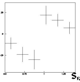
we got the distribution shown in Fig. 134. We can see a strong phase variation of about 1800 around the mass for theσ(500), showing a phase motion compatible with a re-sonance.
Figure 13. Phase motionδ(s13)distribution for the scalar low mass
ππamplitude, with the errors.
4
Conclusions
We showed that the AD method can be applied to E791 data to extract the phase motion of the resonancef0(980)in the
Dalitz plot of the decayD+
s → π−π+π+ . This example
demonstrates the ability of this method to extract the phase motion of a resonance amplitude.
Preliminary E791 results present a direct and model-independent approach, obtained with the AD method, and confirms our previous result of the evidence of an impor-tant contribution of the isoscalarσ(500)meson inD+ →
π−π+π+ decay [1]. We use the well knownf
2(1270)
ten-sor meson in the crossing channel, as the base resonance, to extract the phase motion of the low massππscalar ampli-tude. We obtain aδ(s13)variation of about 1800consistent
with a resonantσ(500)contribution. We also obtain good agreement between the FSIγcorrobserved with AD method
and theγobserved in the full Dalitz plot analysis.
References
[1] E791 Collaboration, E.M. Aitala et al., Phys. Rev. Lett. 86, 770 (2001).
[2] I. Bediaga and J. Miranda, Phys. Lett. B550, 135 (2002). [3] E791 Collaboration, E.M. Aitala et al., Phys. Rev. Lett. 89,
121801 (2002).
[4] Particle Data Group, Hagiwara et al., Phys. Rev. D 66, 010001-1 (2002).
[5] Carla G¨obel for E791 collaboration, this proceeding and hep-ex/0307003.
[6] Peter Minkowski and Wolfgang Ochs, hep-ph/0209225. To ap-pear in the proceeding of QCD 2002 Euroconference, Mont-pellier 2-9 July 2002.
[7] J. A. Oller, hep-ph/0306294. To appear in the proceeding of Workshop on the CKM Unitarity Triangle, IPPP Durham, April 2003.
[8] A. D. Polosa, hep-ph/0306298. To appear in the proceeding of Workshop on the CKM Unitarity Triangle, IPPP Durham, April 2003.
[9] E791 Collaboration, E.M. Aitala et al., Phys. Rev. Lett. 86, 765 (2001).
[10] J.A. Appel, Ann. Rev. Nucl. Part. Sci. 42, 367 (1992); D.