Rev. Bras. Econ. vol.57 número2

(1)

Maria Cristina T. Terra**

Summary: 1. Introduction; 2. The data and pattern of finance; 3. Econometric analysis; 4. Conclusion.

Keywords: credit constraints; brazilian firms; panel data.

JEL codes: D21; G31; C23.

This paper investigates whether Brazilian firms’ investment deci-sions are affected by credit constraints, using balance sheet data from 1986 to 1997. Estimated results indicate that Brazilian firms are credit-constrained, and the only instance in which credit con-straints seemed softer was among large and among multinational firms, during the period 1994-97.

Este artigo investiga se as decisões de investimento das firmas brasileiras são afetadas por restri¸cões ao crédito, usando dados de balan¸co de firmas entre 1986 e 1997. Os resultados emp´ıricos in-dicam que as firmas brasileiras sofrem de restri¸cão a crédito, e que os únicos casos em que a restri¸cão teve efeito mais suave ocorreram entre grandes firmas e multinacionais, no per´ıodo entre 1994 e 1997.

1. Introduction

In a world with no missing markets, no informational asymmetries and no transaction costs, credit supply and demand should be equalized by an appropri-ate interest rappropri-ate level, with no need for a financial sector. A vast literature, both theoretical and empirical, studies the effects on the economy when these condi-tions do not hold. In the real world, information asymmetries and transaction costs for acquiring information create the need for a financial system. The role

*_{This paper was received in may 2000 and approved in june 2002. I am grateful for helpful}

comments and suggestions from Jose Fanelli, Saul Keifman, Na´ercio Menezes and seminar partic-ipants at the IDRC workshop on Finance and Changing Patterns in Developing Countries, FEA

– Universidade de S˜ao Paulo, and the PRONEX seminar held at Getulio Vargas Foundation. I

thank Patr´ıcia Gon¸calves, from IBRE, Getulio Vargas Foundation, for kindly furnishing data on Brazilian firms’ balance sheets, Carla Bernardes, Pedro Aledi Portugal and, particularly, Cristiana Vidigal for superb research assistance. Financial support from IDRC is gratefully acknowledged. I also thank CNPq for a research fellowship.

**_{Graduate School of Economics, Funda¸c˜}_{ao Getulio Vargas.}

(2)

444 _{Maria Cristina T. Terra}

of the financial sector is then, in summary, to allocate savings to the best invest-ment projects, to monitor managers, and to diversify risk (see Levine (1997) for a discussion on the roles of the financial system). In such an environment, financial system imperfections create credit restrictions, which in turn may affect firms’ investment decisions.

There is an ample literature that seeks empirical evidence of credit constraints by looking at the firm’s investment decision. (For surveys on the subject, see, for example, Hubbard (1998) and Schiantarelli (1996). Bond and Van Reenen (1999) survey more broadly microeconometric research on investment and employment, including their theoretical underpinnings.) This paper uses one of the methodolo-gies advanced by this literature to investigate whether Brazilian firms’ investment decisions are affected by credit constraints. More specifically, this paper examines the cash flow sensitivity in a sales accelerator investment demand model. The intuition for this test is the following. If the estimated investment demand model captures all relevant variables that guide investment decisions, cash flow should not affect investment. However, if the firm is credit constrained, then investment decision is affect by the firm’s cash flow.

One of the advantages of using firm data, instead of aggregated data, is that it allows investigating distinct behavior among different types of firms. This paper explores this feature by studying the behavior of alternative groupings of firms, so that we can compare firms considereda priori to be subject to stronger financial constraints, with those considered to have more access to financial markets. This is a common practice in this literature. (See, for example, Fazzari, S. M. et al. (1988) and Whited (1992)). The groupings of firms used in this paper are large and small firms, multinational and domestic firms, and firms more and less dependent of external finance. The first two divisions are common in the literature, but the last one has never been used before. The division into subgroups should be based on criteria that are correlated neither to investment nor to cash flow. The external finance dependence used in this paper is the criterion that better fits this requirement.

This paper also explores an alternative approach to the cash flow sensitivity test. In a credit-constrained environment, more access to credit should boost investment in more external finance dependent firms. Hence, instead of including cash flow in the investment equation, we include a term that tries to capture whether firms that are more dependent on external funds and that have more access to credit do invest more. The description of this novel approach is presented in section 3.

(3)

the pattern of finance of Brazilian firms. Section 3 estimates investment equations to capture the effects of credit constraints. Section 4 concludes.

2. The Data and Pattern of Finance

The data set comprise balance sheet data for firms that are required by law to publish them. The data were collected by IBRE (Instituto Brasileiro de Economia, Getulio Vargas Foundation) from Gazeta Mercantil and Di´ario Oficial, from 1986 to 1997, with the number of firms in each year ranging from 2,091 to 4,198. From the original sample, those firms which had data published for all years considered were selected1 _{– from 1986 to 1997}2 _{– a total of 550 firms. Non-industrial firms}

were excluded, as well as those with missing data. The sample used is composed of 468 firms, broken down by sector as indicated in table 1.

Table 1 Data Description

Average value of assets* Sector Number of firms (1994 to 1997) Apparel and Footwear 16 151,226,212

Beverages 15 599,900,102

Chemicals Products 71 814,435,409

Drugs 11 137,409,771

Eletric Equipment 28 338,754,575

Food Products 70 170,390,346

Furniture 4 35,992,189

Leather 3 19,429,112

Machinery 38 176,597,031

Metal Products 60 606,166,766

Non-metal Products 30 371,050,142

Other Industries 9 92,482,669

Paper and Products 19 857,736,540

Perfumery and Soap 3 24,547,019

Plastic Products 8 74,543,359

Printing and Publishing 11 97,283,390

Rubber Products 1 17,969,577

Textiles 40 121,148,883

Tobacco 1 409,941,742

Transport Equipment 23 256,891,434

Wood Products 7 252,427,396

* In 1996 constant Reais.

1_{This procedure may bias the sample of firms used, but I argue that the possible bias should}

not favor the result investigated here. I am trying to identify whether firms are credit-constrained. It is plausible to believe that firms which survived throughout the period studied should not be more credit-constrained ones. Hence, if this (possibly) biased sample presents credit constraints, the unbiased sample should also be credit-constrained

2_{The data have two breaks over time, one in 1990 and the other in 1994, due to changes}

(4)

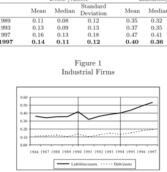
The analysis starts with a description of the firms’ patterns of finance. Two leverage measures are calculated: the ratio between liabilities and assets, and the ratio between debts and assets.3 Figure 1 presents evolution of debts and assets for the whole sample of firms’ averages, and table 2 presents the averages across subperiods: from 1986 to 1989, from 1990 to 1993, and from 1994 to 1997. Over the first period, liabilities and debts were stable in relation to total asset ratios, averaging 35% and 11%, respectively. There was a slight increase in both measures during the second period. Firms were clearly becoming more leveraged over the last period, 1994–1997, when liabilities averaged 47% and debts 16% of total assets.

Table 2 Pattern of finance

Debts /Assets Liabilities/Assets Mean Median _DeviationStandard Mean Median _DeviationStandard

1986 – 1989 0.11 0.08 0.12 0.35 0.32 0.17

1990 – 1993 0.13 0.09 0.13 0.37 0.35 0.18

1994 – 1997 0.16 0.13 0.18 0.47 0.41 0.41

1986 – 1997 0.14 0.11 0.12 0.40 0.36 0.21

Figure 1 Industrial Firms

0,00 0,10 0,20 0,30 0,40 0,50 0,60

86 87 88 89 90 91 92 93 94 95 96 97

Liabilities/Assets Debt/Assets 0.00

1 9 8 6

Liabilities/assets Debt/assets 1 9 9 7 1 9 9 6 1 9 9 5 1 9 9 4 1 9 9 3 1 9 9 2 1 9 9 1 1 9 9 0 1 9 8 9 1 9 8 8 1 9 8 7 0.60

0.50

0.40

0.30

0.20

0.10

The set of firms is divided into subgroups, trying to identify possible differences in finance patterns across different groupings or across different time periods. The subgroup division is based on a priori hypothesis with respect to firms’ credit access. It is reasonable to assume that larger firms would have more access to credit markets than smaller ones. As Gertler and Gilchrist (1994, p. 313) argue, “ while

3_{The measure for debt is the long- and short-term loans on the firm’s balance sheet. Liabilities}

(5)

size per se may not be a direct determinant [of capital market access], it is strongly correlated with the primitive factors that do matter. The informational frictions that add to the costs of external finance apply mainly to younger firms, firms with a high degree of idiosyncratic risk, and firms that are not well collateralized. ... These are, on average, smaller firms.” The finance pattern evolution for those two groups of firms is indeed interesting, as shown in figures 2a and 2b. Although leverage measured as liabilities as a share of total assets does not differ between the two groups of firms, the debts to assets ratio is quite different between them. Large firms have higher debts to assets ratio throughout the whole time frame, compared to small firms.

Figure 2

Debts/Assets

0,05 0,10 0,15 0,20 0,25

86 87 88 89 90 91 92 93 94 95 96 97

Large Firms Small Firms

a b

Liabilities/ Assets

0,30 0,40 0,50 0,60

86 87 88 89 90 91 92 93 94 95 96 97

Large Firms Small Firms

0.60

0.50

0.40

0.30

Large firms Small firms Liabilities/assets

0.25 0.20 0.15 0.10 0.05

Large firms Small firms Debts/assets

19868788899091929394959697 19868788899091929394959697

There are two alternative explanations for the higher indebtedness of large firms compared to that of small firms. Low indebtedness for small firms may be either the result of pure financial decisions or an indication of the credit restrictions they face. If the first alternative is true, some firms simply chose to use fewer external loans, and those are coincidentally the small ones. If the latter is true, a group of firms was credit-restricted, and therefore it was not possible for them to be more leveraged. The empirical exercise performed in section 3 tries to identify which explanation is more consistent with the data.

(6)

external finance for U.S. industries.

Table 3 External dependence

Apparel and Footwear 0.03

Beverages 0.08

Chemicals Products 0.25

Drugs 1.49

Eletric Equipment 0.77

Food Products 0.14

Furniture 0.24

Leather −0.14

Machinery 0.45

Metal Products 0.24

Non-metal Products 0.06

Other Industries 0.47

Paper and Products 0.18

Perfumery and Soap 0.47

Plastic Products 1.14

Printing and Publishing 0.2

Rubber Products 0.23

Textile 0.4

Tobacco −0.45

Transport Equipment 0.31

Wood Products 0.28

Source: Rajan and Zingales (1998)

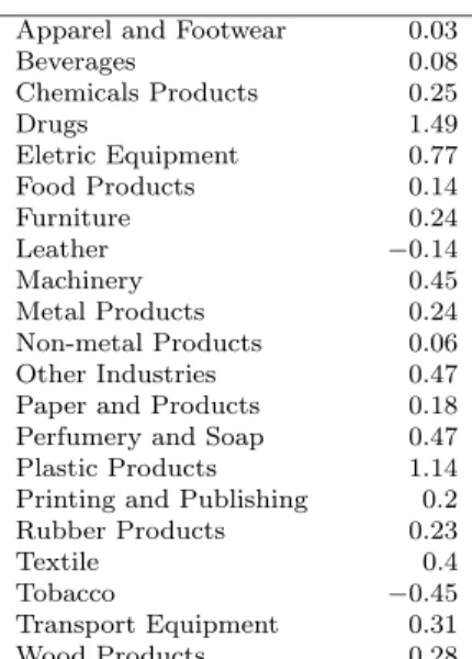
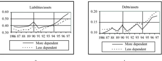
By using the measure constructed in that paper, which is reproduced in table 3, firms have also been divided according to their external dependence: firms in the sectors exhibiting more external dependence have been separated from those firms in sectors presenting less finance dependence.4 It is interesting to note that in Brazil, as figure 3a shows, more financially dependent firms are on average more leveraged than less financially dependent firms, looking at the ratio of liabilities to assets5. That is, firms more in need of external finance according to the external dependence measure exhibit greater use of external finance. With respect to the debts to assets ratio, there is no systematic difference between these two groups: in some periods firms in less dependent sectors have a higher debts to assets ratio, compared to more dependent ones; in other periods they have a lower measure (figure 3b).

4_{Firms which are less dependent on external finance are those in the following sectors:}

Furni-ture, Chemical Products, Wood Products, Transport Equipment, Textiles, Machinery, Perfumery and Soap, Electric Equipment, Plastic Products, Drugs; and Other Industries.

5_{Note that Rajan and Zingales external dependence measure refers to all sorts of external}

(7)

Figure 3

Debts/Assets

0,10 0,15 0,20

86 87 88 89 90 91 92 93 94 95 96 97

More Dependent Less Dependent a b Liabilities/Assets 0,30 0,40 0,50 0,60

86 87 88 89 90 91 92 93 94 95 96 97

More Dependent Less Dependent 0.60 0.50 0.40 0.30 Less dependent Liabilities/assets More dependent 0.20 0.15 0.10 Less dependent Debts/assets More dependent 19868788899091929394959697 19868788899091929394959697

Finally, the sample of firms is divided between multinational and domestic firms. The motivation for this division is that multinational firms may have more access to international credit markets, and therefore they may be less credit-constrained. In both leverage measures, figures 4a and 4b show higher leverage for multinational firms until 1993, and higher leverage for domestic firms from then on. Figure 4 Debts/Assets 0,05 0,10 0,15 0,20

86 87 88 89 90 91 92 93 94 95 96 97 Domestic Firms Multinational Firms Liabilities/Assets 0,30 0,40 0,50 0,60

86 87 88 89 90 91 92 93 94 95 96 97 Domestic Firms Multinational Firms a b 0.60 0.50 0.40 0.30 Multinational firms Liabilities/assets Domestic firms 0.20 0.15 0.10 0.05 Multinational firms Debts/assets Domestic firms 19868788899091929394959697 19868788899091929394959697

3. Econometric Analysis

Fazzari, S. M. et al. (1988) was the first of several papers to estimate invest-ment demand models including cash flow as an independent variable to determine the extent to which firms are credit constrained. The reasoning is that if firms are not credit-constrained, their cash flow variations should not affect investment decisions, after investment opportunities are controlled for. The general form for the investment equations they estimate is:

(8)

where:

Iit andKit represent investment and capital stock of firmiat timet;Xrepresents

a vector of variables affecting firms’ investment decisions, according to theoretical considerations; and uit is an error term. In some specifications, theQ investment

model is estimated by using Tobin’s q as the vector X, and including the cash

flow variable in the equation. In other specifications, the accelerator model of

investment is used, and theX vector is replaced by contemporaneous and lagged

sales to capital ratios.

Using a different method, Whited (1992) estimates Euler equations for an optimizing investment model under two different assumptions: when firms are credit-constrained, and when they are not. Gertler and Gilchrist (1994), on a different approach, study whether small and large firms respond differently to monetary policy. They find that smaller firms have a much stronger response to monetary tightening than larger firms, indicating they are more credit-constrained. All these studies use data for U.S. firms.

The accelerator model specification from Fazzari, S. M. et al. (1988) will be re-produced for Brazilian data to identify the existence (or not) of credit constraints.6 The empirical exercises performed here are based on the sales accelerator invest-ment demand model, where investinvest-ment is explained by current and past sales. Cash flow is included as an explanatory variable for investment, as shown in the equation:

(I/K)it=βi+β0(S/K)it+β1(S/K)i,t−1+α(CF/K)it+uit

where:

Sit represents the sales of firm iat time t. Cash flow should not be a significant

explanatory variable for investment, except when firms are credit-constrained.

That is, the parameter α should not be significant for firms that are not

credit-constrained, and it should be positive and significant for credit-constrained firms.

Table 4 presents the initial results. The first estimation method used was OLS, and the results are in columns (1)–(3). These regressions include firm-specific effects and time dummies for each year, but the coefficients are not reported. First, the investment accelerator model is estimated without including cash flow as an explanatory variable. The best specification for our data is the one including

6_{It is very difficult to use the Euler equation approach, as in Whited (1992), or the}_Q_model

(9)

one lag of the sales variable. As column (1) of table 4 shows, variations in the sales variables explain 53% of investment changes. When cash flow is included in the regression (column (2)), independent variables explain 82% of investment variations, and cash flow has a positive and significant coefficient (witht-statistics of 10.35). According to our conjecture, this is an indication that firms were credit-constrained over the time period studied. All regressions were also estimated in first differences7, and the results were qualitatively similar to the ones reported here.

One should note, however, that the period under study encompasses two dis-tinct situations with respect to capital inflows. From 1986 to 1994 there was very little external capital inflow into Brazil, and from 1994 to 1997 current account deficits increased substantially, reaching 4% in 1997. It is possible that the higher capital inflow increased the credit supply, therefore lessening firms’ credit con-straints. A slope dummy for cash flow for the period 1994–97 has been included in the regression. This variable equals cash flow and capital ratio for the years 1994 to 1997, and is zero for the rest of the period. If firms were less credit-constrained over 1994–1997, this slope dummy should not be positive. That is not the case though, as shown in table 4 column (3). The slope dummy coefficient is posi-tive, with a t-statistic of 2.29. Thus, there is no evidence that firms became less credit-constrained over the period with high external capital inflow.

A major problem with the OLS estimation is that it does not provide a consis-tent estimator when the independent variable is endogenous. Hence, if there are other variables that affect simultaneously investment and cash flow, or investments and sales, then the OLS estimator will not be consistent. The solution is then to use instrumental variables for the independent variables, and to estimate by the method of moments. The equation was estimated in levels and in first differences, using lagged values for cash flow and for sales as instruments for these variables, and the results are presented in columns (7)–(12) of table 4. We have also com-puted a dynamic OLS (columns (4)–(6) of table 3), to make the results comparable with the GMM. It is very interesting to note that both the sign and magnitude of the coefficients are very similar in all regressions presented in table 4. In sum: the coefficient for cash flow is positive and significant, indicating that firms are credit constrained, and the cash flow slope dummy for the period 1994–1997 is also positive and significant, presenting no indication that credit constraints were lessened over the period.

(10)

4

5

2

M

ar

ia

C

ris

tin

a

T

.

T

er

ra

Table 4

Regression results for the whole sample Dependent variable: investment

OLS Dynamic GMM GMM in first

Independent variable OLS differences

and summary statistics

(1) (2) (3) (4) (5) (6) (7) (8) (9) (10) (11) (12) (I/K)_i,t

−1 −0.215 −0.101 −0.101 −0.138 −0.056 −0.051 −0.518 −0.221 −0.321

(−7.517) (−6.699) (−6.397) (−6.740) (−2.600) (−2.740) (−40.79) (−3.41) (−4.19)

(CF /K)_it 1.355 0.871 1.344 0.851 1.454 0.653 1.357 0.845

(10.347) (3.665) (10.267) (3.669) (5.850) (2.320) (4.57) (2.400)

CF /Kslope dummy 0.576 0.575 1.073 1.055

1994–1997 (2.036) (2.086) (4.280) (2.890) (S/K)i,t −0.263 −0.111 −0.100 −0.264 −0.113 −0.103 −0.267 −0.111 −0.082 −0.269 −0.122 −0.067

(−3.567) (−5.163) (−4.617) (−3.613) (−5.408) (−4.869) (−2.820) (−2.960) (−2.270) (−2.54) (−2.91) (−1.73)

(S/K)_i,t

−1 0.284 0.103 0.087 0.258 0.093 0.078 0.239 0.128 0.098 0.122 0.140 0.136

(3.526) (3.514) (3.385) (3.391) (3.450) (3.309) (3.130) (3.180) (3.950) (1.910) (3.420) (3.010)

R2 0.527 0.818 0.827 0.545 0.822 0.831

F-statistic 7.100 66.050 41.830 27.380 118.670 89.190 84.630 676.560 597.190 4344.680 7524.950 9790.410 Number of 468 468 468 468 468 468 468 468 468 468 468 468 firms

Number of 4212 4212 4212 4212 4212 4212 4212 4212 4212 3744 3744 3744 observations

(11)

The next step is to investigate possible differences in credit constraint across groups of firms, based on a priori hypothesis with respect to firms’ credit accessi-bility. The subgroup divisions used here are the ones described in section 2. We start by splitting the sample according to firm size, and the regression results are presented in table 5. The regression was estimated using OLS, dynamic OLS, GMM, and GMM in first differences. Like the results from the whole sample re-gressions, the different methods of estimation yielded similar results. Cash flow coefficients are positive and significant for both groups of firms, in all estimation methods. The coefficient is somewhat larger for the group of large firms in all regressions. As for the cash flow slope dummy for the period 1994–97, it was positive in the case of smaller firms, and not significantly different from zero for larger firms. Therefore, there is no indication of less credit constraints over the period, for both groups.

Instead of splitting the sample into subgroups, another specification was used, which will be denoted here as “slope dummy specification”. In this specification, slope dummies for a subgroup of firms are included in the regression, which are equal to cash flow for the alternative grouping of firms, and zero otherwise. These slope dummies should capture differences in the cash flow coefficient for the differ-ent subgroups of firms. One advantage of this specification compared to estimating separate regressions for each subgroup is that it provides a statistical test for the difference of the cash flow coefficient for the different subgroups. Hence, we will be able to check whether the bigger cash flow coefficient for large firms found in table 5 is significantly different from the coefficient for small firms.

(12)

4

5

4

M

ar

ia

C

ris

tin

a

T

.

T

er

ra

Table 5

Regression results for large and small firms Dependent variable: investment

and summary statistics Large firms Small firms Large firms Small firms Large firms Small firms Large firms Small firms (1) (2) (3) (4) (5) (6) (7) (8) (9) (10) (11) (12) (13) (14) (15) (16) (I/K)_i,t

−1 −0.057 −0.06 −0.106 −0.103 0.027 0.024 −0.064 −0.058 −0.053 −0.089 −0.23 −0.342

(−1.458) (−1.603) (−6.511) (−5.931) (0.510) (0.470) (−2.77) (−2.78) (−1.05) (−1.65) (−3.22) (−4.80)

(CF /K)_it 2.07 1.847 1.326 0.845 2.064 1.821 1.298 0.824 2.122 1.724 1.44 0.614 2.036 1.835 1.318 0.757

(4.893) (7.671) (8.427) (3.624) (4.837) (7.501) (8.293) (3.624) (6.020) (6.490) (4.740) (2.230) (10.860) (7.030) (3.960) (2.360)

CF /Kslope dummy 0.242 0.616 0.264 0.608 0.454 1.194 0.337 1.26

1994 – 1997 (0.615) (2.065) (0.684) (2.093) (1.180) (5.960) (0.530) (4.900) (S/K)it 0.293 0.302 −0.122 −0.117 0.291 0.301 −0.123 −0.119 0.319 0.346 −0.131 −0.121 0.27 0.331 −0.129 −0.102

(1.540) (1.502) (−6.698) (−6.653) (1.523) (1.491) (−6.875) (−6.822) (2.000) (2.000) (−4.63) (−5.34) (2.410) (1.780) (−3.32) (−3.45)

(S/K)_i,t

−1 −0.273 −0.283 0.11 0.097 −0.288 −0.299 0.1 0.087 0.133 0.129 0.126 0.089 0.351 0.386 0.138 0.102

(−1.496) (−1.457) (3.827) (3.751) (−1.623) (−1.580) (3.892) (3.769) (1.730) (1.650) (2.890) (3.300) (3.790) (3.320) (2.870) (3.130)

R2 0.873 0.873 0.805 0.818 0.873 0.874 0.810 0.823

F-statistic 33.60 38.63 56.93 51.03 37.86 39.18 91.21 84.85 185.64 194.21 579.35 745.58 475.87 711.89 6810.81 9241.13 Number of 75 75 393 393 75 75 393 393 75 75 393 393 75 75 393 393 firms

Number of 675 675 3537 3537 675 675 3537 3537 675 675 3537 3537 600 600 3144 3144 observations

(13)

Table 6

and summary statistics (1) (2) (3) (4) (5) (6) (7) (8) (I/K)i,t−1 −0.103 −0.100 −0.055 −0.050 −0.225 −0.328

(−6.89) (−6.35) (−2.63) (−2.63) (−3.23) (−4.52)

(CF/K)it 1.327 0.857 1.301 0.836 1.444 0.635 1.334 0.814 (8.640) (3.660) (8.520) (3.670) (4.910) (2.280) (4.080) (2.45)

CF/Kslope dummy 0.601 0.595 1.167 1.178

1994–1997 (2.030) (2.060) (5.730) (4.280)

CF/Kslope dummy 0.087 0.475 0.103 0.462 0.045 0.578 0.195 0.643 for large firms (0.347) (2.710) (0.414) (2.680) (0.140) (3.050) (0.500) (2.600)

CF/Kslope dummy −0.507 −0.477 −0.840 −0.959

for large (−1.63) (−1.56) (−2.41) (−2.35)

firms 1994–1997

(S/K)it −0.107 −0.102 −0.109 −0.104 −0.108 −0.097 −0.110 −0.081

(−6.29) (−6.18) (−6.49) (−6.38) (−4.25) (−4.91) (−3.24) (−3.08)

(S/K)i,t−1 0.100 0.088 0.090 0.078 0.129 0.093 0.149 0.119

(3.770) (3.670) (3.750) (3.660) (3.070) (3.740) (3.200) (3.480)

R2 _0.819 _0.828 _0.823 _0.832

F-statistic 53.54 50.11 89.66 79.73 670.69 733.86 7685.44 10452.16

Number of 468 468 468 468 468 468 468 468

firms

Number of 4212 4212 4212 4212 4212 4212 4212 4212 observations

Note: The dependent variable is investment-capital ratio. TheCF/Kslope dummy is a vari-able that has value equal toCF/K for the years 1994 to 1997, and zero in all. Regressions (1)–(6) were estimated using firms’ fixed effects, but the coefficients are not other years repor-ted. For regressions (7)–(8), all variables are in first differences, and there are no dummies for firms. All regressions were estimated using year dummies for every year, but the coefficients are not reported. Thet-statistics in parentheses are based on White heteroskedasticity-consis-tent standard errors.

When a cash flow slope dummy for the period 1994–97 is included (columns (2), (4), (6), and (8)), we find that the cash flow coefficient for that period is lower in large firms, although also positive and significant.8 _{The cash flow coefficient}

for large firms in the period 1994–97 is negative and significant in the GMM and GMM in first differences specifications. This can be an indication that large firms are less credit constrained than smaller one over the period from 1994 to 1997. Figures 2a and 2b from section 2 showed that large firms have higher debt to assets ratio compared to small firms. The result from the regressions in table 6 indicate that the difference in indebtedness between the two groups of firms may be due to discriminated access to credit only over the period 1994–97.

8_{The cash for coefficient for large firms during the period 1994–1997 is the sum of the}

(14)

4

5

6

M

ar

ia

C

ris

tin

a

T

.

T

er

ra

Table 7

Regression results for multinational and domestic firms Dependent variable: investment

OLS differences

Independent variable Multinational firms Domestic firms Multinational firms Domestic firms Multinational firms Domestic firms Multinational firms Domestic firms and summary statistics (1) (2) (3) (4) (5) (6) (7) (8) (9) (10) (11) (12) (13) (14) (15) (16) (I/K)_i,t

−1 −0.13 −0.128 −0.092 −0.088 −0.066 −0.067 −0.056 −0.049 −0.062 −0.036−0.227 −0.349

(−3.731) (−3.712) (−5.075) (−4.488) (−1.17) (−1.20) (−2.39) (−2.40) (−1.55) (−0.81) (−3.19) (−5.03)

(CF /K)it 1.158 1.322 1.461 0.887 1.139 1.250 1.436 0.869 1.587 1.561 1.499 0.622 1.890 2.016 1.338 0.732

(5.827) (5.896) (8.167) (3.699) (5.849) (5.409) (7.987) (3.701) (7.560) (5.560) (4.770) (2.220) (12.550) (10.730) (3.970) (2.340)

CF /Kslope −0.174 0.738 −0.118 0.731 0.036 1.264 −0.189 1.354

dummy 1994 – 1997 (−0.666) (2.294) (−0.451) (2.314) (0.130) (6.090) (−0.93) (5.210)

(S/K)_it −0.112 −0.117 −0.127 −0.121 −0.119 −0.122 −0.129 −0.122 0.087 0.091 −0.14 −0.129 −0.239 0.211−0.139 −0.109

(−1.187) (−1.193) (−6.289) (−6.241) (−1.288) (−1.277) (−6.426) (−6.368) (0.770) (0.780) (−4.42) (−5.06) (2.750) (2.310) (−3.33) (−3.53)

(S/K)i.t−1 0.087 0.087 0.112 0.097 0.064 0.065 0.103 0.088 0.059 0.058 0.128 0.088 0.277 0.272 0.131 0.092

(1.481) (1.472) (3.705) (3.593) (1.102) (1.098) (3.686) (3.601) (0.770) (0.760) (2.790) (3.160) (2.860) (2.840) (2.700) (2.820)

R2 0.923 0.923 0.798 0.815 0.926 0.926 0.802 0.818

F-statistic 922.44 741.55 44.66 39.88 839.36 704.87 97 89.04 773.15 788.9 585.42 632.11 1398.21 1465.8 6238.53 8509.88 Number of 46 46 422 422 46 46 422 422 46 46 422 422 46 46 422 422 firms

Number of 414 414 3798 3798 414 414 3798 3798 414 414 3798 3798 368 368 3376 3376 observations

(15)

International credit markets may also be more accessible for multinational firms, compared to domestic ones. Table 7 present the results for the regressions estimated for multinational and domestic firms separately. Here again, all cash flow coefficients are positive and significant, indicating credit constraints for both groups. The cash flow slope dummy for the period 1994–97 is positive and signifi-cant for domestic firms, and not statistically different from zero for multinationals.

Table 8

and summary statistics (1) (2) (3) (4) (5) (6) (7) (8) (I/K)i,t−1 −0.096 −0.093 −0.055−0.049 −0.221 −0.332

(−5.76) (−5.15) (−2.54) (−2.54) (−3.11) (−4.60)

(CF/K)it 1.449 0.890 1.423 0.871 1.497 0.632 1.359 0.798 (8.300) (3.720) (8.127) (3.720) (4.880) (2.260) (4.070) (2.42)

CF/Kslope dummy 0.718 0.711 1.246 1.269

1994–1997 (2.260) (2.280) (5.970) (4.570)

CF/Kslope dummy for −0.280 0.253 −0.265 0.234 −0.182 0.535 −0.007 0.495

multinational firms (−1.59) (1.090) (−1.510) (1.020) (−0.63) (2.330) (−0.02) (1.570) CF/Kslope dummy for −0.681 −0.644 −1.050 −1.051

multinational firms (−2.21) (−2.10) (−3.79) (−2.91)

1994–1997

(S/K)it −0.124−0.118 −0.126 −0.119 −0.121−0.109 −0.122 −0.090

(−6.43) (−6.35) (−6.58) (−6.49) (−4.50) (−5.27) (−3.39) (−3.36)

(S/K)i,t−1 0.110 0.094 0.100 0.085 0.127 0.088 0.140 0.109

(3.770) (3.650) (3.740) (3.650) (2.950) (3.520) (3.000) (3.220)

R2 _0.822 _0.835 _0.825 _0.827

F-statistic 147.37 103.49 182.77 136.97 739.74 752.42 7520.89 9991.24 Number of firms 468 468 468 468 468 468 468 468 Number of 4212 4212 4212 4212 4212 4212 4212 4212 observations

Note: The dependent variable is investment-capital ratio. TheCF/Kslope dummy is a variable that has value equal toCF/Kfor the years 1994 to 1997, and zero in all other years. Regressions (1)–(6) were estimated using firms’ fixed effects, but the coefficients are not reported. For regressions (7)–(8), all variables are in first differences, and there are no dummies for firms. All regressions were estimated using year dummies for every year, but the coefficients are not reported. Thet-statistics in parentheses are based on White heteroskedasticity-consistent standard errors.

(16)

4

5

8

M

ar

ia

C

ris

tin

a

T

.

T

er

ra

Table 9

Regression results for more dependent and less dependent firms Dependent variable: investment

OLS differences

Independent variable More dependent Less dependent More dependent Less dependent More dependent Less dependent More dependent Less dependent and summary statistics firms firms firms firms firms firms firms firms

(1) (2) (3) (4) (5) (6) (7) (8) (9) (10) (11) (12) (13) (14) (15) (16) (I/K)_i,t

−1 −0.142 −0.139 −0.076 −0.076 −0.092−0.091 −0.031−0.028 −0.291−0.394 −0.131 −0.179

(−5.632) (−5.202) (−4.505) (−4.412) (−2.94) (−2.82) (−1.88) (−1.73) (−3.70) (−5.46) (−3.43) (−3.07)

(CF /K)it 1.022 0.642 1.601 1.268 0.995 0.619 1.584 1.25 1.092 0.428 1.801 1.186 0.978 0.534 1.797 1.522

(6.078) (2.940) (9.457) (6.377) (6.036) (2.961) (9.360) (6.317) (3.100) (1.900) (10.710) (4.290) (2.720) (1.910) (11.540) (5.620)

CF /Kslope dummy 0.515 0.37 0.51 0.371 1.061 0.731 1.154 0.473

1994 – 1997 (1.703) (1.410) (1.765) (1.432) (7.650) (2.260) (6.500) (1.160) (S/K)_it −0.113 −0.106 −0.063 −0.056 −0.117 −0.11 −0.065 −0.058 −0.122 −0.109 −0.021 0.005 −0.108−0.082 −0.061 −0.025

(−5.136) (−5.191) (−1.276) (−1.131) (−5.619) (−5.627) (−1.364) (−1.214) (−3.28) (−4.14) (−0.26) (0.060) (−2.09) (−2.20) (−0.72) (−0.35)

(S/K)i,t−1 0.124 0.105 0.048 0.046 0.114 0.095 0.039 0.037 0.156 0.102 0.099 0.106 0.188 0.127 0.118 0.145

(2.643) (2.515) (1.665) (1.589) (2.712) (2.603) (1.341) (1.263) (2.580) (2.710) (2.800) (2.860) (4.300) (4.830) (1.460) (1.840)

R2 0.781 0.796 0.853 0.855 0.79 0.804 0.855 0.857

F-statistic 29.73 28.8 44.25 36.99 58.15 59.37 103.39 86.22 470.98 394.93 537.65 559.54 5225.51 5769.61 4052.28 4808.05 Number of firms 179 179 289 289 179 179 289 289 179 179 289 289 179 179 289 289 Number of 1611 1611 2601 2601 1611 1611 2601 2601 1611 1611 2601 2601 1432 1432 2312 2312 observations

(17)

inflow seems to have lessened only multinational firms’ credit constraint.

The sample is also split according to external dependence, using Rajan’s and Zingales’ (1998) measure, and the estimated regressions are presented in table 9. The cash flow coefficients are positive and significant in all regressions, but they are higher for less-dependent firms. The results from the slope dummy specification, in columns (1), (3), (5), and (7) of table 10, show that the cash flow coefficient for more dependent firms is significantly smaller than that of less dependent firms. One interpretation is that less-dependent firms would use less external finance, therefore their investment would be more cash flow sensitive. The cash flow slope dummy for more dependent firms 1994–97 is not significantly different from zero in all regressions presented in table 10.

Table 10

and summary statistics (1) (2) (3) (4) (5) (6) (7) (8) (I/K)i,t−1 −0.098−0.098 −0.048 −0.048 −0.179 −0.266

(−6.67) (−6.37) (−2.95) (−2.89) (−4.06) (−4.53)

(CF/K)it 1.527 1.158 1.505 1.135 1.677 1.053 1.547 1.112 (9.030) (6.720) (9.040) (6.630) (9.340) (4.700) (7.580) (4.06)

CF/Kslope dummy 0.415 0.417 0.763 0.871

1994–1997 (1.660) (1.700) (2.470) (2.100)

CF/Kslope dummy −0.436 −0.472 −0.431−0.465 −0.488 −0.534 −0.614−0.944

for more (−2.07) (−1.87) (−2.09) (−1.88) (−1.46) (−2.05) (−1.71) (−4.26)

dependent firms

CF/Kslope dummy 0.116 0.114 0.345 0.570

for more dep. (0.330) (0.330) (1.120) (1.460) firms 1994–1997

(S/K)it −0.097 −0.090 −0.100−0.093 −0.089 −0.074 −0.109−0.062

(−4.72) (−4.46) (−5.01) (−4.74) (−2.66) (−2.24) (−2.64) (−1.73)

(S/K)i,t−1 0.095 0.082 0.085 0.073 0.129 0.097 0.154 0.139

(3.730) (3.480) (3.640) (3.360) (3.690) (4.350) (3.400) (3.270)

R2 _0.827 _0.834 _0.831 _0.838

F-statistics 35.64 30.03 98.72 82.45 837.44 858.00 6912.93 9333.45 Number of 468 468 468 468 468 468 468 468 firms

Number of 4212 4212 4212 4212 4212 4212 4212 4212

Note: The dependent variable is investment-capital ratio. TheCF/Kslope dummy is a variable that has value equal toCF/Kfor the years 1994 to 1997, and zero in all other years. Regressions (1)–(6) were estimated using firms’ fixed effects, but the coe-fficients are not reported. For regressions (7)–(8), all variables are in first differences, and there are no dummies for firms. All regressions were estimated using year dumm-ies for every year, but the coefficients are not reported. Thet-statistics in parentheses are based on White heteroskedasticity-consistent standard errors.

(18)

do-460 _{Maria Cristina T. Terra}

mestic firms, more and less externally dependent. The only instances of credit-constraint reduction was among large and among multinational firms, from 1994 to 1997.

3.1 Further Results

Kaplan and Zingales (1997) argue that investment-cash-flow sensitivities do not provide a useful measure of finance constraints, introducing controversy re-garding the validity of this methodology. An alternative empirical exercise is then performed, without the use of cash flows, motivated by Rajan and Zingales (1998). Rajan and Zingales (1998) investigate the effect of financial sector development on industrial growth. Their main hypothesis is that “ industries that are more de-pendent on external financing will have relatively higher growth rates in countries that have more developed financial markets” (p. 562). They use industry-level data for several countries to estimate an equation where industry growth is ex-plained by the interaction between an industry’s external dependence and the country’s financial development, controlling for country indicators, industry indi-cators, and that industry’s share in the country’s economy. That is, they have an equation that tries to capture possible variables that explain differences in in-dustry growth rates in different countries, and they include a new variable in the equation, namely external dependence multiplied by financial development. Their conjecture is that if financial development is indeed important for growth, the co-efficient of this interaction variable should be positive: more dependent industries would tend to grow faster in a more financially developed environment.

We borrow this idea from Rajan and Zingales (1998) in the following way. In a financially constrained environment, more dependent firms that have access to credit should be relatively better off. Less dependent firms, on the other hand, should not be much affected by credit access. Hence, when explaining cross-firm investment levels, more dependent firms would tend to invest more when they have more access to credit, in a credit-constrained environment.

(19)

the dynamic OLS (column (2)), using GMM with lagged variables as instruments (column (3)), and estimating GMM in first differences (column (4)).9

Table 11

Dynamic GMM in first

Independent variable OLS OLS GMM differences

and summary statistics (1) (2) (3) (4)

(I/K)i,t−1 −0.218 −0.139 −0.518

(−7.544) (−6.82) (−40.86)

Interaction (external 341.118 396.247 1008.555 1032.721 dependenceXfirm size) (2.673) (3.055) (2.630) (2.450)

(S/K)it −0.264 −0.265 −0.269 −0.270

(−3.587) (−3.367) (−2.86) (−2.57)

(S/K)i,t−1 0.282 0.255 0.238 0.120

(3.536) (3.402) (3.130) (1.880)

R2 _0.528 _0.546

F-estatistic 5.690 20.550 92.400 4351.290

Number of firms 468 468 468 468

Number of 4212 4212 4212 3744

observations

Note: The dependent variable is investment-capital ratio. Regressions (1)–(3) were estimated using firms’ fixed effects, but the coefficients are not reported. For regression (4), all variables are in first differences, and there are no dum-mies for firms. All regressions were estimated using year dumdum-mies for every year, but the coefficients are not reported. Thet-statistics in parentheses are based on White heteroskedasticity-consistent standard errors.

In this empirical specification, it makes no sense to divide the sample of firms into large and small firms, because the criteria used for such divisions is already contained in the new independent variable used. An alternative grouping of firms is used, based on asset growth. One group, denoted “winners” , is composed of those firms that presented an above average asset growth rate over the period, and the other group, “losers”, is composed of firms with asset growth rate below average. The interaction term (external dependence times firm size) is positive and significant in both subgroups, in all estimation methods used, as shown in table 12. It is interesting to note, though, that the coefficient is more than four times larger for the group of loser firms.

9_{All regressions were also estimated including firm size as explanatory variable. The coefficient}

(20)

Table 12

Regression results for winner and loser firms Dependent variable: investment

OLS Dynamic OLS GMM GMM in first

Independent variable Winners Losers Winners Losers Winners Loosers differences and summary statistics (1) (2) (3) (4) (5) (6) (7) (8) (I/K)i,t₋1 −0.184 −0.248 −0.103 −0.185 −0.509 −0.528

(−4.108) (−7.070) (−4.90) (−6.58) (−34.32) (−23.97) Interaction (external 228.119 899.059 266.012 979.178 850.925 1415.94 870.038 1348.42 dependenceXfirm size) (2.385) (2.907) (2.693) (2.890) (2.100) (2.650) (1.920) (2.730) (S/K)it −0.288 −0.257 −0.284 −0.26 −0.314 −0.256 −0.308 −0.257 (−4.223) (−2.845) (−4.270) (−2.912) (−3.35) (−2.23) (−3.20) (−1.92) (S/K)i,t₋1 0.28 0.28 0.252 0.252 0.218 0.225 0.123 0.112

(4.416) −2.665 −4.084 (2.569) (4.230) (2.340) (2.280) (1.120)

R2 _0.51 _0.546 _0.522 _0.570

F-statistic 11.26 3.63 12.20 17.76 91.40 69.86 3269.11 1886.59

Number of firms 235 233 235 233 235 233 235 233

Number of 2115 2097 2115 2097 2115 2097 1880 1864

observations

Note: The dependent variable is investment-capital ratio. TheCF/Kslope dummy is a varia-ble that has value equal toCF/Kfor the years 1994 to 1997, and zero in all other years. Re-gressions (1)–(6) were estimated using firms’ fixed effects, but the coefficients are not reported. For regressions (7)–(8), all variables are in first differences, and there are no dummies for firms. All regressions were estimated using year dummies for every year, but the coefficients are not reported. Thet-statistics in parentheses are based on White heteroskedasticity-consistent sta-ndard errors.

Table 13

Dynamic GMM in first Independent variable OLS OLS GMM differences and summary statistics (1) (2) (3) (4) (I/K)i,t−1 −0.218 −0.139 −0.517

(−7.557) (−6.85) (−41.08)

Interaction (external 900.35 978.96 1485.82 1274.83 dependenceXfirm size) (2.690) (2.840) (2.670) (2.360) Interaction slope −701.63 −730.97 −638.9 −489.52

dummy for winners (−2.18) (−2.20) (−0.93) (−0.72)

(S/K)it −0.263 −0.263 −0.268 −0.269

(−3.61) (−3.66) (−2.86) (−2.55)

(S/K)i,t−1 0.281 0.254 0.238 0.123

(3.550) (3.420) (3.120) (1.950)

R2 _0.529 _0.547

F-statistc 4.310 16.500 95.250 4440.080

Number of firms 468 468 468 468

Number of 4212 4212 4212 3744

observations

Note: The dependent variable is investment-capital ratio. TheCF/K slo-pe dummy is a variable that has value equal toCF/Kfor the years 1994 to 1997, and zero in all other years. Regressions (1)–(6) were estimated using firms’ fixed effects, but the coefficients are not reported. For regres-sions (7)–(8), all variables are in first differences, and there are no dumm-ies for firms. All regressions were estimated using year dummdumm-ies for every year, but the coefficients are not reported. Thet-statistics in parentheses are based on White heteroskedasticity-consistent standard errors.

(21)

an interaction term slope dummy for winner firms. The results, presented in table 13, show that the coefficient for the interaction term slope dummy is negative and significant in the OLS regression. This means that the interaction coefficient for

winner firms is lower than for loser firms, although both are positive.10 In the

GMM regressions, however, the interaction term slope dummy coefficient is not significantly different from zero, indicating no difference in the behavior of those two groups of firms.

4. Conclusion

This paper investigated credit constraints in Brazil using firm’s balance sheet data. The empirical analysis tried to answer two key questions: whether firms’ investment decisions are affected by credit constraints, and whether credit con-straints differ among different groups of firms. Following a well-established trend in the empirical literature, an investment accelerator model was estimated, in-cluding cash flow as an explanatory variable. The model posits that if firms are not credit-constrained, the cash flow coefficient should not be a significant, once investment determinants are controlled for. According to the estimated results, Brazilian firms are indeed credit-constrained. The only instance in which credit constraints seemed softer was among multinational and among large firms, during the 1994-97 period.

Additionally, an alternative approach to the cash flow-sensitivity model was applied. The investment accelerator model was re-estimated, this time including an interactive term between external dependence and credit access. The results show that firms more in need of external financing and with more access to credit tend to invest more.

All told, both methodologies clearly indicate that Brazilian firms operate under credit constraints in their investment decisions.

References

Bond, S. & Van Reenen, J. (1999). Microeconometric models of investment and employment. mimeog.

Fazzari, S. M., Glenn, R. H., & Petersen, B. C. (1988). Financing constraints and

corporate investment. Brookings Papers on Economic Activity, 1:141–206.

10_{Remember that the effect of the interaction term on winner firms should equal the sum of}

(22)

Gertler, M. & Gilchrist, S. (1994). Monetary policy, business cycle, and the

behav-ior of small manufacturing firms. Quarterly Journal of Economics, 109(2):309–

40.

Hubbard, R. G. (1998). Capital-market imperfections and investment. Journal of

Economic Literature, XXXVI:193–225.

Kaplan, S. & Zingales, L. (1997). Do investment cash flow sensitivities provide

useful mearsures of financing constraints? Quarterly Journal of Economics.

Levine, R. (1997). Financial development and economic gowth: Views and agenda.

Journal of Economic Literature, XXXV:688–726.

Rajan, R. G. & Zingales, L. (1998). Financial dependence and growth. The

American Economic Review, 88(3):559–86.

Schiantarelli, F. (1996). Financial constraints and investment: Methodological issues and international evidence. Oxford Review of Economic Policy, 12(2):70– 89.

Whited, T. M. (1992). Debt, liquidity constraints, and corporate investment: