Choice: Application to Brazilian States
Wilfredo L. Maldonado
∗
, Isabel M. Marques
†
, Osvaldo C. da
Silva Filho
‡
Contents: 1. Introduction; 2. Costs and Returns of Education; 3. A Dynamic Model of School Choice; 4. The Stationary States and Their Stability; 5. Conclusion; A. Appendix I; B. Appendix II;
Keywords: Education Level Choice, Non-Concave Dynamic Programming, Multiplicity of Equilibria.
JEL Code: C62, D91, J31.
Using the education level/wage distribution curve of the Brazilian States we define a dynamic programming problem to determine the optimal choice of education level of the parents in their descendants favor. As aproxyfor the opportunity cost of education we use the public expenditure in education. The results show that low level educated workers will use public schools to provide education to their offspring. For high educated workers (which receive higher wages) we find the existence of several steady states, some of them stable and others unstable. The findings point out the concentration of education in some specific levels and the existence of a poverty trap, where low educated workers chose low level of education for their descendants perpetuating low wages for the familiar unit. The performed exercise may be used as subside to the definition of public educational policies.
Utilizando a curva de distribuição de salários por nível de educação dos Estados Brasileiros, definimos um problema de programação dinâmica para determinar o nível de educação ótimo que os pais escolhem para os seus descendentes. Comoproxypara o custo de oportunidade da educação utilizamos os gastos públicos em educação. Os resultados mostram que trabalhadores com nível de escolaridade baixo devem recorrer a escolas públicas para proporcionar educação aos seus filhos. Por outro lado, para
∗Graduate School of Economics, Catholic University of Brasilia, Brazil. Corresponding author. Address: SGAN 916, Módulo B. Brasília DF. CEP 70790-160. Brazil. Phone/Fax: (55)(61)3448-7127. This author would like to thank the financial support provided by CNPq (Brazil) through grants 300954/2006-9 and 401461/2009-2. This research was concluding during a visiting academic period of the author to the Research School of Economics in the Australian National University. E-mail:[email protected] †National Confederation of Industry, Brazil.
trabalhadores com alto nível de escolaridade (os quais recebem maiores salários) encontramos a existência de vários estados estacionários, alguns deles estáveis e outros inestáveis. Os resultados apontam a concentração de educação em alguns níveis específicos e a existência da armadilha da pobreza, onde trabalhadores com baixa escolaridade somente conseguem oferecer baixa escolaridade aos seus filhos e portanto perpetuando um nível baixo de salários para a unidade familiar. O exercício realizado pode ser útil para subsidiar a definição de políticas públicas de educação.
1. INTRODUCTION
A study performed by Barros et alii (2000) emphasizes that education and its returns are responsible for nearly half of the wage inequality in Brazil. An explanation for this may be found in the increasing demand of more skilled workers experienced in the country especially in the 90’s when the Brazilian economy was growing, spurred on by companies using sophisticated but stable technology. In this way, the scarcity of high skilled workers and that the demand for them result in a greater disparity in income between those with education and those without it. This disparity in incomes is the exact outcome observed in Brazil, especially after the 90’s, due to trade openness.
From a theoretical point of view, Becker e Tomes (1979) formulated a model of intergenerational transmission of inequality of income, including investment of parents in the education of their children. They showed that while the transmission of the family “gifts” like financial or human capital are not very large, the families will go up and down, and back to average income within a few generations.
Regarding the level school choice Becker (1962) shows that it is an economic decision that weighs the costs and the benefits of the attained level of education. Therefore it has to take into account the remuneration evolution of an employee during the production cycle, the turnover between jobs, the large investment in education and the wage increases during the life cycle among the most educated workers. Later on Becker (1994) argues that in addition to improvements in wages and occupations, the benefits include greater stability and other non-monetary gains (status).
A final observation comes from the modern theory of human capital. It asserts that there are characteristics or “attributes” that determine personal productivity and as a result, the wage. The theory assumes that each individual receives exactly the value of its marginal productivity and this is related to a set of personal characteristics. Such characteristics may be education, experience and income and education of parents (Malan e Wells, 1973).
In this vein, this work analyzes the dynamics of school level choice in a dynamic programming problem where the individual chooses the current consumption and the school level that he/she will give to his/her offspring. The returns of the education level (education level/wage curve) are exogenously taken and from empirical observation. The shape of that curve does not correspond to a concave function, thus a non-concave dynamic programming problem arises because of it. As a consequence we obtain an optimal policy function which may have more than one stationary state. Some of them may be repellent and others may be attractors. This result explains the prevalence of polarization in the levels of education (and in wages as a consequence) and therefore the existence of the poverty traps. The study is applied to the Brazilian States of the Federation. At the end of this paper we display these stationary states and analyze their stability properties.
To construct the education level/wage curve we use the average wage data from the National Household Sample Survey (PNAD)1for the year 2009. To model the expenditure function of schooling we
used as aproxythe government spending (Federal, State and Municipal) given by the National Institute
for Educational Studies and Research (INEP/MEC).2It seems to be a reliableproxysince we will not model
explicitly the government and we will use a representative agent.
Our model and methodology may be used as a subsidy to the definition of public policies in the Education Sector. For instance, increasing public expenditures in high levels of education would imply a reduction in the cost of education of households and would modify the stationary levels of education of future generations. Analogously, given the low wages that low level educated workers exhibit it might be worth implement or reinforce the “Bolsa Escola” program (subsidy received by low-income families conditioned to the permanence of the children at the school).
Our theoretical model was inspired by that of Nishimura e Raut (2007). They consider a dynamic programming problem where the altruistic head of the family chooses the quality of the school of his offspring and consequently the possibility of intergenerational social mobility. They conclude that the existence of many qualities of school implies a non-concave earning function for the children; in this way, many steady-state equilibria emerge. With that result they are able to explain the existence of “poverty trap” which are attractor states with low income levels. The difference between their work and ours is that we do not deal with quality matters but with the possibility of children concluding, or not, a given level of education. Furthermore, our earning function depends on the level of education (which is an empirical fact observed in Brazil) and not on the quality of it.
This paper is organized as follows: after this introduction we make a brief discussion on the costs and returns of education (Section 2). In Section 3 we describe the dynamic model of school choice. In Section 4 we report the computed steady states of education and present an analysis of their stability in the long-run using the iterations of the optimal policy function. Finally, Section 5 contains the main conclusions. The calibration of the marginal costs of education is reported in the Appendix 1 and the optimal policy functions defining the school level choices in each Brazilian State are shown in the Appendix 2.
2. COSTS AND RETURNS OF EDUCATION
Langoni (1974) showed that in the decades of 1960 and 1970 Brazil exhibit high rates of returns on education. Recently, Barbosa Filho e Pessoa (2008) updated the Langoni findings and showed that initial education has an internal rate of return larger than 15%. But the highly educated worker not only has a higher wage but a lower chance of being unemployed. In Brazil, an individual with less than eight years of schooling had a probability of 17.6% of being unemployed in 2002. After finishing high school (eleven years of schooling) his chances of unemployment fell to 10.9%. If he had begun but never finished university, the chances of unemployment were only 5.4%. Thus, investment in education not only has higher returns in terms of wages, but also has non-monetary returns. Guarantee of employment is one of these.
The fundamental idea is that labor is more than just a production factor. It should be considered as a type of capital: human capital. This capital may increase and become more productive if the owner invests through education. That investment makes the human capital more functional and capable to follow the technological innovations.
The theory of human capital was incorporated in modern economic theory by Jacob Mincer, and “popularized” by Schultz (1960), Schultz (1961) and Becker (1962). According to Mincer (1958) investment in education should be seen as an economic decision. The well known Mincerian equations relate the wage of a worker with the years of schooling he has, his experience and other explanatory variables.
Despite all the benefits and high returns of education it is observed that developing economies exhibit non-negligible portions of population with low levels of education. The explanation is not
difficult: parents with low levels of schooling have low wages, so the opportunity cost of their children’s education is high. For individuals with more education the opposite is true. Thus, it is not surprising to obtain two (or more) stationary levels of schooling, as found in this article.
Therefore, a correct model to analyze the optimal dynamic decision of schooling must include the structure of the returns of education (the education level/wage function) and the cost specification of education. It will be done in the next section.
3. A DYNAMIC MODEL OF SCHOOL CHOICE
In this section we present the main ingredients of the dynamic model of schooling choice. After that, we describe the model itself and solve it in order to find the equilibrium.
3.1. Returns of schooling
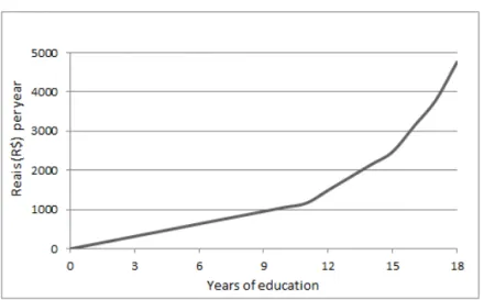
Using the PNAD 2009 database we analyze the wage structure depending on the level of schooling in Brazil. We perceived that the education level/wage curve presents a non-concave function shape in all the Brazilian States. Figure 1 depicts the shape of the (mean) wage curve for the Brazilian States.3 The
horizontal axis represents the school level4and the vertical one is the relative wage with respect to the
highest wage in the State. It is worth noting that the return of schooling, measuring in terms of wages, has low increasing returns (and in some cases even decreasing returns) for the first years of education (elementary and incomplete secondary school). After concluding the secondary school education the curves experience a rapid increase until reaching the complete higher education (undergraduate and graduate studies). In some States the wage received by incomplete Master degree studies is lower than the previous level of education, but after completing those high levels of education it is pushed to highest values. We should notice that in some cases (Maranhão – MA, Paraíba – PB and Alagoas – AL in the Northeast and Espírito Santo – ES in the Southeast), education levels higher than the Master degree reduces the mean wage in the State, displaying an S-shaped curve (corresponding to a convex-concave function) of education/wage distribution. Later on we will show that such behavior in the curve will induce individuals with high education to offer lower levels of education to their descendants.
We may provide two explanations for the shape of the above curves. In Brazil (like in other countries) the so called “diploma effect” triggers a sensible increase in salaries. An individual with an incomplete secondary school level receives a much lower and flatter wages than one with a complete secondary school. Workers with incomplete elementary school receive (almost) the same wage, because the labor market does not distinguish among them. On the other hand individuals with the highest levels of education (graduate level or more) are almost equally remunerated for an analogous reason. The second explanation comes from a theoretical point of view. If education is a mechanism of signaling in a labor market with adverse selection, a separating equilibrium will produce a convex-concave education level/wage curve (Spence, 1973, 1974).
From now on, we will represent byw(e)the annual wage of an individual witheyears of education.
3.2. Education expenditure function
Using the database reported by the National Institute for Educational Studies and Research (INEP / MEC) we consider as aproxyfor educational expenditure the Government expenditure in education5for
3The State name corresponding to each acronym is given in the Appendix 1.
4The number “0” represents illiterate; “1” is one year of schooling and so on until “12”. The number “16” represents complete
graduate studies; “17” is the complete Master degree studies, and “18” is more than master degree studies.
5The expanded data for the States available from INEP is for 2008, thus we apply as a correction the inflation rate given by the
Figure 1: Education/wage curve – Brazilian States
each of the 18 levels of schooling we are considering. Depending on the State, it might be a lower bound for the education expenditure, since private schools charged annuities greater than those reported in the database above. In any case, what we are trying to represent is the opportunity costs of having a child in the school, and that costs increases piecewise linearly, depending on the age of the child.
A particular characteristic of the data is that for each of the first 11 years of education (elementary and secondary school) the expenditure in each year does not vary significantly. Expenditures rise for each year of university education and more (from the 12th to the 22nd). Therefore we will assume a piecewise linear function to represent the educational expenditure function. Namely, ifk1 >0is the
average cost of each year of education for the first 11 years andk2>0is the average cost of each year
of education from the 12th on, then the educational expenditure function is:
g22(e) = (
k1e if e611
k2e+ 11(k1−k2) if 11< e622
. (1)
We are using the subscript “22” to indicate the expenditure when considering 22 years of education. The constantsk1andk2are calibrated in order to obtain an annual expenditure in education for a family
which invest in schooling of a number of sons equal to the fertility rate during a period of 20 years. Due to the aggregation of the data available from the PNAD, we identify levels 16, 17 and 18 as being 17, 19 and 22 year of education respectively. Making this aggregation we will obtain the functiong(e)which defines the expenditure for those new 18 levels of education.6 The calibrated parameters are reported
in Appendix 1. Figure 2 shows the shape of education expenditureg(e)of the considered levels for the Federal District (DF).
Figure 2: Annual education expenditure – DF
Source: Elaborated by the authors.
3.3. The education level choice model
Using the education level/wage curve and the education expenditure function described above, we will define the dynamic programming problem whose solution will provide the optimal schooling level
6Namely,g(e) =g
choice function. Let us consider an individual who is choosing his current consumption and what he will spend on the education level of his descendant. The individual has an education levele0 >0and
thus a wage given byw(e0). The utility function for current consumption is given byU :R+→Rand
it is the same for all his descendants. The degree of altruism shown towards his son is given by the discount factorβ ∈ (0,1). Therefore, the problem which defines the optimal individual consumption and the education level choice for the descendants is:
v(e0) = max
{ct,et+1} +∞ t=0
+∞
X
t=0
βtU(ct)
s. t. ct+g(et+1) =w(et) (2) e0∈E= [0,18]
The dynamic programming problem (2) expresses the assumption of an individual level of education affects or determines the offspring level of education. That assumption was widely tested in Brazil (Barros (1997), Barros et alii (2001)) and abroad (Daouli et alii (2010), Bauer e Riphahn (2007), Behrman e Rosenzweig (2002), Black et alii (2005)).
The objective function in (2) is the classical separable one. It is important to notice that although the choice of consumption is for all the period of life (that we will consider as being 20 years), we can consider the budget constrain in a yearly basis (using the yearly average consumption, wages and educational expenditures). However, the discount factor should be measured for the total period of life.
To solve the problem (2) we will use the associate Bellman equation: v(e0) = max
e∈[0, g−1(w(e 0))]
U(w(e0)−g(e)) +βv(e) (3)
Despite the functions we are going to use are not differentiable, it might be useful consider the differentiable case in order to get some intuition of the marginal conditions defining the optimal consumption and education level choice. Thus, if the functions included in (2) are differentiable, a very intuitive relationship may be obtained from the Euler equations. Namely, if the optimal path e0,e∗1,e∗2,· · · is an interior solution, then:
−U′(w(et−1)−g(et))g′(et) +βU′(w(et)−g(et+1))w′(et) = 0. (4) From (4), a very natural condition may be obtained:
βU′(c
t) U′(c
t−1) = g
′(e
t) w′(e
t) ,
which is the equality between the intertemporal marginal rate of substitution and the marginal real cost of education. It means that the willingness to substitute current consumption for future consumption must be equal to the net gain of increasing the level of the off-springs’ education.
To solve numerically equation (3) we will use the contraction mapping theorem applied to the operator T f(e0) = maxe∈[0,g−1(w(e
0))]U(w(e0)−g(e)) +βf(e)which generates a sequence of
value function approximations vn+1 = T vn. Once a tolerance level is attained an approximationvˆ is selected. Finally, with thatvˆwe can obtain an optimal policy function approximation by:
φ(e0) = max
e∈[0,g−1(w(e 0))]
U(w(e0)−g(e)) +βvˆ(e)
Before making the estimation of the value function and the correspondent policy function, it will be useful to analyze the existence of stationary steady states for the problem.
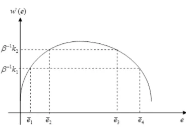
holde∗t = ¯efor allt, and therefore w
′(¯e) = β−1g′(¯e). If wis a convex-concave function, its first
derivative has an increasing-decreasing shape. On the other hand, due to the piecewise linearity ofg, its first derivative must assume more than one value (for simplicity, suppose two: β−1k
1andβ−1k2),
depending on the education level. Figure 3 shows the possible steady states.
Figure 3: Multiple steady states
Notice that this approach only detects interior steady states where the return functionU(w(e0)−
g(e1))is differentiable. The optimal policy function will report the remaining steady states.
To estimate the value function we proceed by using the iterative method described above. The numerical inputs are as follows. The education level/wage curve and the education expenditure function are defined as described in subsections 3.1 and 3.2. We use a CRRA utility functionU(c) =
c1−γ/(1−γ), whereγ = 4.89and annual discount factor 0.9,7 values reported by Issler e Piqueira
(2000). For this value ofγ, the return functionU(w(e0)−g(e1))is not bounded. However, we can
use the Theorem 4.14 of Stokey e Lucas (1989, p. 92); in this way, we guarantee that the solution of the Bellman equation is, in fact, the value function. The accuracy of the optimal policy function is guaranteed by the strong concavity of the return function, as stated by Maldonado e Svaiter (2007).
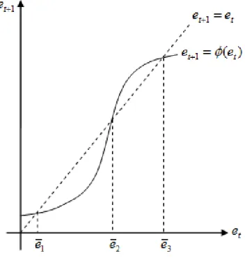
In the next section we will report the steady states for each Brazilian State and in the Appendix 2 we present the optimal policy function. As we will see, there exists multiplicity of steady states. It might be useful to illustrate de dynamics evolution around those steady states and how it results in the existence of polarization in education and in the poverty trap. To this end, Figure 4 shows an example of the shape of an optimal policy function with three stationary states.
The modulus of the derivative of the optimal policy function evaluated in each steady state provides information about its stability. For instance, as the modulus of the derivative is lower than one ine¯1
and ¯e3 it results the local stability of such states. On the other hand, the derivative of the optimal
policy function evaluated in¯e2has modulus greater than 1 and so is locally unstable. Thus, in the long
run, initial states in the interval(0,e¯2)will converge toe¯1and initial states in the interval(¯e2,18)will
converge toe¯3.
This result reveals a perverse polarization in the education level: poor people will select a low level of education for their offspring and rich individuals (or at least those with high levels of education)
7Therefore we will useβ= 0.920
Figure 4: Optimal policy function in education level choice: Multiplicity of steady states
will select a high level of education for their descendants. Such polarization of education implies a polarization of wages which is an observed phenomenon in the USA (Rosenthal, 1985) and in Brazil (Scorzafave e Castro, 2007). The “poverty trap” which results from that polarization is not a surprising outcome. Individuals endowed with a low education level have low wages and the opportunity cost of providing more education to their children is relatively too high when compared with the marginal increase in the future wages. For this reason they prefer to maintain the descendants out of school. On the other side of the coin, a person with a high level of education, in addition to having a relatively high salary, has a small opportunity cost of providing more education to his descendants (because of the decreasing marginal utility). This result is a strong argument for the implementation of public policies of conditional income transfers, which enforce the maintenance of children in the school.
4. THE STATIONARY STATES AND THEIR STABILITY
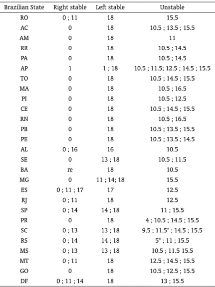
In Appendix 2 we provide the optimal policy function of education level choice for each Brazilian State. Table 1 summarizes all the stationary states and their stability properties. In that Table we say that a stationary state is “Right stable” if initial higher levels of education in a near interval will regress to that stationary state; a stationary state is “Left stable” if it attracts lower levels of education in a near interval of it and a stationary state is said “Unstable” if levels of education in a near interval around it are moved away from it. The “∗” mark represents a stationary state which attracts an isolated level of education which is not close to it.
As we may observe, the illiteracy is a strong attractor for the first levels of education in all States. This may be comprehended since a worker with low school levels of education receive very low wages, then the opportunity cost of education is high, thus naturally they would prefer to keep the descendants out of the school. Therefore, those workers rely on public education or even in conditional income transfers to maintain the children at the school. A tenuous exemption is observed in Amapá (AP), where the attractor is one year of school education.
Table 1: Stationary states and their stabilities
Brazilian State Right stable Left stable Unstable RO 0 ; 11 18 15.5 AC 0 18 10.5 ; 13.5 ; 15.5
AM 0 18 11
RR 0 18 10.5 ; 14.5 PA 0 18 10.5 ; 14.5 AP 1 1 ; 18 10.5 ; 11.5; 12.5 ; 14.5 ; 15.5 TO 0 18 10.5 ; 14.5 ; 15.5 MA 0 18 10.5 ; 16.5
PI 0 18 10.5 ; 12.5 CE 0 18 10.5 ; 14.5 ; 15.5 RN 0 18 10.5 ; 16.5 PB 0 18 10.5 ; 13.5 ; 15.5 PE 0 18 10.5 ; 13.5 ; 14.5 AL 0 ; 16 16 10.5 SE 0 13 ; 18 10.5 ; 11.5 BA re 18 10.5 MG 0 11 ; 14; 18 15.5 ES 0 ; 11 ; 17 17 12.5 RJ 0 ; 11 18 12.5 SP 0 ; 14 14 ; 18 11 ; 15.5 PR 0 18 4 ; 10.5 ; 14.5 ; 15.5 SC 0 ; 13 13 ; 18 9.5 ; 11.5* ; 14.5 ; 15.5 RS 0 ; 14 14 ; 18 5* ; 11 ; 15.5 MS 0 ; 13 13 ; 18 10.5 ; 11.5 15.5 MT 0 ; 11 18 12.5 ; 14.5 ; 15.5 GO 0 18 10.5 ; 12.5 ; 15.5 DF 0 ; 11 ; 14 18 13 ; 15.5
the cost of providing a high level of education to the descendant is also high, the low marginal utility of consumption makes the worker to be willing to pay for it due to altruistic motivations (represented by the discount factor). In addition, the parsimonious increase of education expenditures for advanced levels of education compared with the high wage that educated worker may attain makes him to invest in the education of his offspring.
Finally, we can observe one or more interior stationary states that are unstable. They determine the intervals where the low and high attracting levels of education act (the basins of attraction).
From the Table 1 we can conclude that low level educated workers (with low income) provide low level of education for their descendants and high level educated workers (therefore with high income) offer high level of education for their offspring. Thus this model explains two phenomena, the so called
poverty trap and thepolarization of education levelsin the society. These two problems were largely documented in the literature, as discussed in former sections.
One interesting exercise may be performed once we have the optimal policy function of education level choice.8Since this is a dynamic model, we may follow the consecutive decisions of education level
choices of future generations, simply iterating the optimal policy function in each State. It is important to notice that:
i) each iteration will correspond to the decision for one generation ahead (20 years, in our case); ii) This is a ceteris paribus simulation, namely, keeping the wage distribution structure and the
education expenditure curve unchanged.
Thus, it is a qualitative simulation just showing the tendencies of the evolution in the school levels distribution.
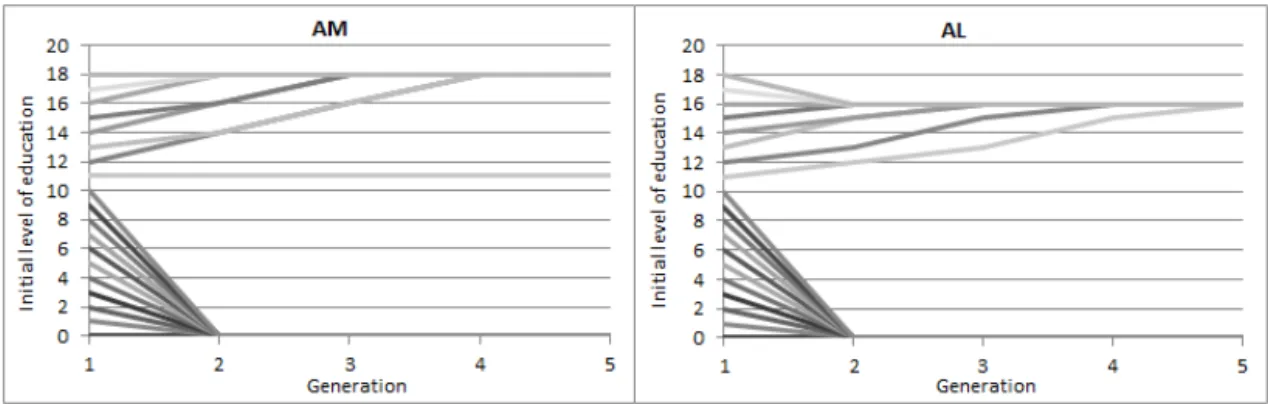
Figures 5 to 8 show the projections of the education levels obtained from the iterations of the optimal policy function for some representative States in each region. We selected those States by either their significance in terms of population or the richness of the dynamics that is being generated.
Figure 5: Evolution of education – North and Northeast
Figure 5 shows that in Amazonas (AM) the transition to the highest level is from education levels greater than the secondary school and we can note that the higher is the level, the faster is the transition. In Alagoas (AL) the evolution is not to the highest level, but to what represents the complete graduate studies. The reason for this is the S-shaped wage curve for that State (see Figure 1), thus the head of the family does not find the highest level as a worth level for his son in terms of schooling returns. Analogous dynamics can be found for the States of Maranhão (MA) and Paraíba (PB). We can also notice that the transition to the highest level is slower than in Amazonas (AM).
Figure 6: Evolution of education – Southeast
Regarding the Southeast region, Figure 6 illustrates that the States of Minas Gerais (MG) and São Paulo (SP) present several stationary states which are right or left stables. Complete secondary school, incomplete graduate studies, complete graduate studies and the highest level of education are attractors. This is explained by the high diversification of economic activities that are available in those States. In Rio de Janeiro (RJ), complete high school and complete post-graduate studies are the major tendencies.
Figure 7: Evolution of education – South
States exhibit for the incomplete high education level (see Figure 1). In SC we can observe the transition to the incomplete undergraduate studies coming from below and above of that level. Nevertheless workers with complete graduate studies may launch also to the highest level of education. In RS we observe the largest amount of attracting levels of education in both directions, increasing the level or decreasing it.
Figure 8: Evolution of education – Central West
Finally, Figure 8 shows the evolutions in Mato Grosso (MT) and Distrito Federal (DF). In the first one the slow transition to the top level of education is observed, however the complete secondary school is also an attractor. Again, due to the decrease of the education returns in the incomplete undergraduate studies, we have that the worker offers a lower level of education to his son, however in the next generations higher levels of education are provided. In the DF, due to the high demand of diverse levels of education to act in the public administration, we can observe the existence of several stationary state attractors.
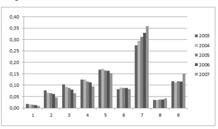
To finalize we provide an empirical observation that supports the existence of attractors in education levels of workers. Using the Annual Report of Social Information (RAIS) database9 we
construct the distribution of education levels in Brazil from 2003 to 2007. For that period, the levels of education are grouped into nine categories that are explained in Table 2.
Table 2: RAIS categories of education levels
Categories Years of Education
1 0
2 1 to 5 Incomplete
3 5
4 6 to 9 Incomplete
5 9
6 10 to 12 Incomplete
7 12
8 13 to 16 Incomplete 9 16 and more
Figure 9 depicts the distributions of education levels for the asserted period. Similar shapes may be obtained for all the Brazilian States. It is possible to observe the slow evolution of that distribution. As time passes, the level of complete secondary school is becoming more populated. A similar behavior is observed for the highest level of education (in a lower intensity). The concentration of workers in those two levels of education is just the dynamics obtained in some of our cases, thus this empirical observation is coherent with our findings.
Figure 9: Education level distribution in Brazil from 2003 to 2007
Source: RAIS (2007).
5. CONCLUSION
The influence of the education level of an individual on that of his descendants is a phenomenon frequently verified through econometric tests in diverse economies. The altruism of the agents with respect to their offspring in addition to the perception of future returns of education is confronted with current consumption decisions. The optimal choice between these two variables is found when each income unit displaced from consumption to the education level of the offspring compensates the returns they will receive in the future.
To apply the model to the Brazilian States of the Federation we calibrated the education returns function using the National Household Sample Survey – PNAD database of 2009 and we used as a
proxyfor the education cost function the public expenditure in education provided in a database from INEP/MEC. With these functions we found the optimal policy functions for the school level choice and compute the stationary states of the education levels for each Brazilian State. Afterwards, we calculate the attractor basins of each stationary state and perform a qualitative analysis of the sequence of the education level optimal choices. The general findings are: workers with incomplete secondary school have no conditions to provide education for their offspring, thus they should appeal to the public education and in addition, it is necessary some sort of conditional income transfer that avoids the school drop out of the children due the high opportunity cost of keeping them into the educational system. It is also shown that in all States there exist (at least) two attractor levels of education, the low level and the high level. Finally, The North States exhibit more concentration in education and as a consequence more inequality coming from the poverty trap. In the Southeast and South States it is observed more than two attractors, which means a higher distribution of school levels, this is due the diversity of economic activities demanding workers with different levels of education. In the Distrito Federal (DF) it is also observed the same characteristic since the public administration also demands individuals with different levels of schooling. For all the States, the optimal policy function provided in the Appendix 2 reveals the attractors basins for each stationary state.
It is worth noting that the results strongly depend on the invariance of the education level/wage curve.10 It is a strong hypothesis to assume that this curve will remain with the same shape for all
generations. The interactions between the skilled and non-skilled labor supply and the demand for those kinds of workers may modify the shape of the wage distribution. A general equilibrium model which captures the feedback between the supply and the demand of these inputs for production would be more realistic to identify a stable shape for the education level/wage relationship.
BIBLIOGRAPHY
Barbosa Filho, F. & Pessoa, S. (2008). Retorno da educação no Brasil. Pesquisa e Planejamento Econômico, 38(1):97–126.
Barros, R. P. d. (1997). A educação e o processo de determinação dos salários no nordeste brasileiro.
IPEA, Working paper.
Barros, R. P. d., Henriques, R., & Mendonça, R. (2000). Education and equitable economic development.
Economia, 1(1):111–144.
Barros, R. P. d., Mendonça, R. Santos, D., & Quintães, G. (2001). Determinantes do desempenho educacional no Brasil. Pesquisa e Planejamento Econômico, 31(1):1–42.
Bauer, P. & Riphahn, R. (2007). Heterogeneity in the intergenerational transmission of educational attainment: Evidence from Switzerland on natives and second-generation immigrants. Journal of Population Economics, 20(1):121–148.
Becker, G. S. (1962). Investment in human capital: A theoretical analysis. Journal of Political Economy, 70.
Becker, G. S. (1994).Human Capital: A Theoretical and Empirical Analysis with Special Reference to Education. University Of Chicago Press, 3rd edition.
10The hypothesis of piecewise linearity of the educational cost is not essential for the result. It is sufficient to have an increasing
Becker, G. S. & Tomes, N. (1979). An equilibrium theory of the distribution of income and intergenerational mobility.Journal of Political Economy, 87(6):1153–89.
Behrman, J. R. & Rosenzweig, M. R. (2002). Does increasing women’s schooling raise the schooling of the next generation? American Economic Review, 92(1):323–334.
Black, S. E., Devereux, P. J., & Salvanes, K. G. (2005). Why the apple doesn’t fall far: Understanding intergenerational transmission of human capital. The American Economic Review, 95(1):pp. 437–449. Daouli, J., Demoussis, M., & Giannakopoulos, N. (2010). Mothers, fathers and daughters:
Intergenerational transmission of education in greece. Economics of Education Review, 29(1):83–93. Issler, J. & Piqueira, N. (2000). Estimating relative risk aversion, the discount rate and the intertemporal
elasticity of substitution in consumption for Brazil using three types of utility function. Brazilian Review of Econometrics, 20(2):201–239.
Langoni, C. (1974). As causas do crescimento econômico do Brasil. J. Olympio.
Malan, P. & Wells, J. (1973). Distribuição da renda e desenvolvimento econômico do Brasil. Pesquisa e Planejamento Econômico, 3(4):1103–1124.
Maldonado, W. L. & Svaiter, B. (2007). Hölder continuity of the policy function approximation in the value function approximation. Journal of Mathematical Economics, 43(5):629–639.
Mincer, J. (1958). Investment in human capital and personal income distribution. Journal of Political Economy, 66(4):281–302.
Nishimura, K. & Raut, L. K. (2007). School choice and the intergenerational poverty trap. Review of Development Economics, 11(2):412–420.
Rosenthal, N. H. (1985). The shrinking middle class: Myth or reality?Monthly Labour Review, 108(3):3–10. Schultz, T. W. (1960). Capital formation by education.Journal of Political Economy, 68:571.
Schultz, T. W. (1961). Investment in human capital.The American Economic Review, 51(1):1–17.
Scorzafave, L. G. & Castro, S. (2007). Ricos? Pobres? Uma análise da polarização da renda para o Brasil 1981-2003. Pesquisa e Planejamento Econômico, 37(2):283–298.
Spence, A. M. (1973). Job market signaling.The Quarterly Journal of Economics, 87(3):355–74.
Spence, M. (1974). Market Signaling: Informational Transfer in Hiring and Related Screening Processes. Cambridge: Harvard UP.
A. APPENDIX I
MARGINAL COSTS OF EDUCATION
IfEi is the total expenditure to reach a school level of educationi, lis the life expectation and n is the fertility rate, thenki = n(Ei/l). Using the database regarding the public expenditure in education reported by the National Institute for Educational Studies and Research (INEP/MEC) for 2008, applying the correction by the Wholesale Consumer Price Index (IPCA) of 2009, the life expectation and the fertility rate from the IBGE database, we obtain the following values forki, i= 1,2:
Table A1: Marginal cost of education (R$ per year)
State Acronym k1 k2
Acre AC 71.79 109.87
Alagoas AL 51.67 119.25
Amapá AM 54.52 93.27
Amazonas AP 81.62 65.98
Bahia BA 49.72 92.52
Ceará CE 50.31 96.42
Distrito Federal DF 106.12 327.07 Espírito Santo ES 80.17 164.15
Goiás GO 65.91 86.09
Maranhão MA 47.54 65.98
Mato Grosso MG 65.02 176.57 Mato Grosso do Sul MS 67.97 150.15 Minas Gerais MT 60.82 127.70
Pará PA 41.36 114.51
Paraíba PB 47.98 112.69
Paraná PE 46.74 103.24
Pernambuco PI 46.21 79.28
Piauí PR 61.71 110.72
Rio de Janeiro RJ 79.61 193.32 Rio Grande do Norte RN 59.31 122.99 Rio Grande do Sul RO 54.24 124.01
Rondônia RR 96.22 103.77
Roraima RS 64.57 214.05
Santa Catarina SC 68.08 125.60 São Paulo SE 62.77 117.72
Sergipe SP 90.86 214.95
B. APPENDIX II
In this Appendix we report the optimal policy functions which define the education level choice of parents to their offspring. We group them by States of the Federation.
Figure A2-4 – Optimal policy functions for the South States – cont.