Time and outcome framing in intertemporal tradeoffs

(1)

Time and Outcome Framing in Intertemporal Tradeoffs

Marc Scholten

ISPA University Institute

Daniel Read

University of Warwick

A robust anomaly in intertemporal choice is the delay–speedup asymmetry: Receipts are discounted more, and payments are discounted less, when delayed than when expedited over the same interval. We developed 2 versions of the tradeoff model (Scholten & Read, 2010) to address such situations, in which an outcome is expected at a given time but then its timing is changed. The outcome framing model generalizes the approach taken by the hyperbolic discounting model (Loewenstein & Prelec, 1992): Not obtaining a positive outcome when expected is a worse than expected state, to which people are over-responsive, or hypersensitive, and not incurring a negative outcome when expected is a better than expected state, to which people are under-responsive, or hyposensitive. The time framing model takes a new approach: Delaying a positive outcome or speeding up a negative one involves a loss of time to which people are hypersensitive, and speeding up a positive outcome or delaying a negative one involves a gain of time to which people are hyposensitive. We compare the models on their quantitative predictions of indifference data from matching and preference data from choice. The time framing model systematically outperforms the outcome framing model.

Keywords: intertemporal choice, discounting, delay–speedup asymmetry, outcome framing, time framing

Intertemporal choices are choices between streams of outcomes differing in value and timing. Psychologists have largely investigated monetary intertemporal choices, such as one between $100 now and $150 in 1 year. This is a decision of whether to accept or decline a 50% interest rate applied to $100 now, or, conversely, of whether to accept or decline a 33% discount rate applied to $150 in 1 year. Psychologists have discovered numerous anomalies to a rational-choice analysis, in which the interest or discount rate implied by choice is constant and equal to the decision maker’s opportunity cost of money. For many people, this is the bank rate of interest or the mortgage rate. However, people are influenced by many characteris-tics of the choice task that are normatively irrelevant.

Every monetary transaction will involve receipts or payments. To determine the interest rate, rational-choice analysis does not care which. Yet, experimental investigations have revealed two robust patterns in which receipts and payments are not treated in the same

way. One result, the gain–loss asymmetry (Loewenstein & Prelec,

1992) or the sign effect (Thaler, 1981), is a main effect of outcome

sign: People offer lower interest rates for payments than they demand

for receipts (Baker, Johnson, & Bickel, 2003; McAlvanah, 2010;

Murphy, Vuchinich, & Simpson, 2001;Xu, Liang, Wang, Li, & Jiang, 2009; Yates & Watts, 1975). Consider the following two choices between a smaller-sooner outcome (SS) and a larger-later one (LL): Receipts: SS Receive $100 today. LL Receive $150 in 1 year. Payments: SS Pay $100 today. LL Pay $150 in 1 year.

Someone who is indifferent between SS and LL for receipts (demanding a 50% interest rate) will typically prefer SS for pay-ments (offering less than 50%). The other result, the delay– speedup asymmetry (Loewenstein & Prelec, 1992), is an interac-tion effect between outcome sign and changes in outcome timing: People demand higher interest rates for delayed receipts than they

offer for expedited ones (Appelt, Hardisty, & Weber, 2011;

Ben-zion, Rapoport, & Yagil, 1989; Loewenstein, 1988; Malkoc & Zauberman, 2006;McAlvanah, 2010;Shelley, 1993;Weber et al.,

2007) and offer lower interest rates for delayed payments than they

demand for expedited ones (Appelt et al., 2011;Benzion et al.,

1989;McAlvanah, 2010;Shelley, 1993). Consider the following pairs of choices for receipts and payments:

Receipts: Delay:

You are entitled to receive $100 today. Choose between:

SS Receive $100 today, as planned.

LL Delay the receipt and receive $200 in 1 year instead.

This article was published Online First January 28, 2013.

Marc Scholten, Department of Social and Organizational Psychology, ISPA University Institute, Lisbon, Portugal; Daniel Read, Warwick Busi-ness School, University of Warwick, Coventry, England.

We acknowledge the financial support from the Fundação para a Ciência e Tecnologia (FCT), Program POCI 2010, and Projects POCI/ PSI/56030/2004, PPCDT/PSI/56030/2004, and PTDC/PSI-PCO/101447/ 2008.

Correspondence concerning this article should be addressed to Marc Scholten, ISPA University Institute, Rua Jardim do Tabaco 34, 1149-041 Lisboa, Portugal. E-mail:[email protected]

This document is copyrighted by the American Psychological Association or one of its allied publishers. This article is intended solely for the personal use of the individual user and is not to be disseminated broadly. 1192

(2)

Speedup:

You are entitled to receive $200 in 1 year. Choose between:

SS Receive $200 in 1 year, as planned.

LL Speed up the receipt and receive $100 today instead.

Payments: Delay:

You are obliged to pay $100 today. Choose between:

SS Pay $100 today, as planned.

LL Delay the payment and pay $120 in 1 year instead.

Speedup:

You are obliged to pay $120 in 1 year. Choose between:

SS Pay $120 in 1 year, as planned.

LL Speed up the payment and pay $100 today instead.

Someone who, for receipts, is indifferent between SS and LL in the delay frame (demanding a 100% interest rate) will typically prefer LL in the speedup frame (offering less than 100%). In a similar vein, someone who, for payments, is indifferent between SS and LL in the delay frame (offering a 20% interest rate) will typically prefer LL in the speedup frame (demanding more than 20%).

“Because,” according toLoewenstein and Prelec (1992, p. 578),

“the two pairs of choices are actually different representations of the same underlying options, the [preference patterns] constitute a classic framing effect, which is inconsistent with any normative theory.” In this article, we examine two alternative interpretations of the delay–speedup asymmetry, one ascribing it to the framing of

outcomes, as is done in previous models (Loewenstein, 1988;

Loewenstein & Prelec, 1992;Shelley, 1993), and the other ascrib-ing it to the framascrib-ing of time.

The gain–loss and delay–speedup asymmetries, however, are not the only anomalies to the normative interest-rate model. To accommodate a broad range of anomalies, many of which are also anomalous to “conventional” models like the discounted

utility model (P. A. Samuelson, 1937), the hyperbolic

discount-ing model (Loewenstein & Prelec, 1992), and the

quasi-hyperbolic discounting model (Laibson, 1997), we developed

the tradeoff model (Scholten & Read, 2010). In this article, we

further develop the tradeoff model to arrive at quantitative predictions of data that contain the gain–loss and delay– speedup asymmetries along with three other anomalies. In par-ticular, we develop two versions of the tradeoff model, one that ascribes the delay–speedup asymmetry to outcome framing, and the other that ascribes it to time framing. The time framing model systematically outperforms the outcome framing model in the prediction of indifference data from matching and pref-erence data from choice.

We begin with the compound-interest model and the expo-nential discounting model deriving from it, which will provide the dependent variables in our analyses of indifference data from matching. The exponential discounting model, along with other discounting models to be specified later in this introduc-tion, will serve as benchmarks to evaluate the predictive accu-racy of the tradeoff models.

Compound Interest Rates

and Exponential Discount Rates

Let xSbe the immediate outcome, and xLbe the outcome that

is delayed by tLunits of time, so that the smaller-sooner (SS)

outcome is (xS, 0) and the larger-later (LL) outcome is (xL, tL).

The interest-rate model posits that the person will be indifferent

between SS and LL when xLis the amount that xSwould become

if increased by the interest over the period tL. Thus, when the

personal interest rate is r, we have:

xS(1⫹ r)tL⫽ xL. (1)

In this model, the person demands compound interest, which is that

interest earned over xSalso bears interest. To illustrate, someone

indifferent between $100 today and $150 in 1 year will also be indifferent between $100 and $225 in 2 years. Solving Equation 1 for the per-period interest rate,

r⫽

冉

xL xS

冊

1⁄tL

⫺ 1. (2)

The compound-interest model describes present-to-future con-version, but it may be changed so as to describe future-to-present conversion instead, which is what the exponential dis-counting model does:

xS⫽ 1

(1⫹ r)tLxL⫽ ␦

t_L

xL, (3)

where 0⬍ ␦ ⬍ 1 is a per-period discount factor, which indicates the

proportion of the (discounted) value of xL that remains over one

period of time. To illustrate, if the person is indifferent between $100 today and $150 in 1 year, the proportion of the $150 receipt that remains over a period of 1 year is 67%. Solving Equation 3 for the per-period discount factor,

␦ ⫽

冉

xS

xL

冊

1⁄tL

. (4)

The per-period discount factor is inversely related to discounting: Lower values indicate more discounting. Instead of looking at how much remains over one period of time, one can look at how much is lost over one period of time. This is what the per-period discount

rate does: It indicates the proportion of the value of xLthat is lost

over one period of time:

␳ ⫽ r

1⫹ r⫽ 1 ⫺ ␦,

where 0⬍ ␳ ⬍ 1 is the per-period discount rate. To illustrate,

if the person is indifferent between $100 today and $150 in 1

year, the rate at which the $150 receipt is discounted is ␳ ⫽

.50/(1⫹ .50) ⫽ 1 – .67 ⫽ .33, that is, the proportion of its value

that is lost over one period of time is 33%. The per-period discount rate is directly related to discounting, in that higher values indicate more discounting.

The exponential discounting model posits that the personal

interest rate r, or the discount fraction␦ and discount rate ␳ into

which the personal interest rate can be transformed, is constant. However, the gain–loss and delay–speedup asymmetries show that r varies. In the next section, we describe three other anomalies to the exponential discounting model that will fea-ture in our data.

This document is copyrighted by the American Psychological Association or one of its allied publishers. This article is intended solely for the personal use of the individual user and is not to be disseminated broadly.

(3)

Anomalies to the Exponential Discounting Model

Two anomalies were described in the introduction: 1. The gain–loss asymmetry or the sign effect, and 2. the delay–speedup asymmetry.

In addition to these sign-related anomalies, we examine anomalies related to the magnitude of the outcomes and the delay to the outcomes, which are described below.

3. The absolute magnitude effect (Loewenstein & Prelec,

1992) or the size effect (see Thaler, 1981): People demand or

offer lower interest rates with large outcomes than with small ones. For instance, someone indifferent between $100 today and $150 in 1 year (50%) might also be indifferent between $1,000 today and $1,250 in 1 year (25%). The absolute mag-nitude effect is probably the most robust anomaly in

intertem-poral choice (Scholten & Read, 2010), and the most difficult

one to address with parametric specifications of discounting

models (Scholten & Read, 2012).

4. The delay effect (Thaler, 1981): People demand or offer

lower interest rates with long delays than with short ones. For instance, someone indifferent between $100 today and $150 in 1 year (50% per annum) might also be indifferent between $100 today and $200 in 2 years (41% per annum). The delay effect is conventionally addressed by hyperbolic discounting models.

Finally, while the delay–speedup asymmetry is an interaction between outcome sign and changes in outcome timing, we also examine its interaction with delay length. This anomaly has not been identified earlier, but we infer it from one piece of avail-able evidence.

5. An attenuation of the delay–speedup asymmetry for longer delays. The evidence comes from Malkoc and Zauberman (2006), who reported an interaction effect between the delay to the larger outcome and changes in outcome timing: The delay effect was stronger when delaying a receipt than when speeding it up. A hypothetical reconstruction of their result is provided in

the top left panel of Figure 1. The dependent variable is the

interest rate r, which, for comparability with subsequent pre-sentations of results, is reversely scaled. We see that r is higher in the delay frame than in the speedup frame, which is the delay–speedup asymmetry for receipts, and that r decreases more sharply with delay length in the delay frame than in the speedup frame, which is the novel result: The strength of the delay effect depends on the frame.

Malkoc and Zauberman (2006)did not examine how their result would generalize to payments, but our prediction is that it will actually reverse for payments: We expect that r will be higher in the speedup frame than in the delay frame, which is the delay–speedup asymmetry for payments, and that r will decrease more sharply with delay length in the speedup frame than in the delay frame, a hypothetical representation of which

is given in the top right panel ofFigure 1.

To see the rationale for our prediction, the bottom panels of

Figure 1represent the same results in a different format, with the respective panels representing short and long delays rather than receipts and payments. What we see is an attenuation of the

delay–speedup asymmetry for longer delays. That is, r generally decreases for longer delays, which is the delay effect, but also becomes less affected by changes in outcome timing, which, according to the tradeoff model, is a corollary of the delay effect.

The Basic Tradeoff Model

Consider a sooner outcome xSdelayed by tSunits of time, and

a larger outcome xLdelayed by tLunits of time. In the present

investigation, we consider only cases where the sooner outcome

is immediate, so that tS⫽ 0. When the outcomes are positive

(e.g., receiving $100 today or $150 in 1 year), SS has an advantage along the time attribute (one will receive 1 year sooner), while LL has an advantage along the outcome attribute (one will receive $50 more). When the outcomes are negative (e.g., paying $100 today or $150 in 1 year), SS has an advantage along the outcome attribute (one will pay $50 less), while LL has an advantage along the time attribute (one will pay 1 year later).

Advantages do not enter the model as differences between raw attribute amounts, but rather as differences between amounts that are transformed to take the psychological impact of time and outcome into account. Specifically, advantages are

differences between weighted delays, w(tL) ⫺ w(0) ⫽ w(tL),

and between valued outcomes, v(xL) ⫺ v(xS) for receipts and

v(xS)⫺ v(xL) for payments. The decision maker will prefer SS

when its advantage is greater than that of LL, prefer LL when its advantage is greater than that of SS, and be indifferent other-wise. The indifference point is given as follows:

␬w(tL)⫽

再

v(xL)⫺ v(xS) if xL⬎ xS⬎ 0

v(xS)⫺ v(xL) if xL⬍ xS⬍ 0,

(5)

where␬ ⬎ 0 is a tradeoff parameter, which scales the difference

between weighted delays and the difference between valued outcomes in a common currency.

The value function v and the time-weighing function w are reference-dependent functions ranging from identity functions,

that is, v(x) ⫽ x and w(t) ⫽ t (constant sensitivity), to zero

functions, that is, v(x) ⫽ 0 for all x, and w(t) ⫽ 0 for all t

(insensitivity). Between these two limits, v and w are concave functions, thus exhibiting diminishing absolute sensitivity (Tversky & Kahneman, 1991): For constant absolute increases of x and t, v(x) and w(t) increase by decreasing absolute amounts. For instance, adding 1 day to a delay of 1 week yields a greater increase in the weight of time than adding 1 day to a delay of 52 weeks. Furthermore, v and w exhibit augmenting proportional sensitivity (Scholten & Read, 2010): For constant proportional increases of x and t, w(t) and v(x) increase by increasing absolute amounts. For instance, doubling $100 yields a greater increase in value than doubling $1. Finally, v exhibits constant loss aversion (Tversky & Kahneman, 1991): Revers-ing the sign of an outcome from positive to negative increases the magnitude of its value by a multiplicative constant, that is,

v(⫺x) ⫽ ⫺␭v(x), where ␭ ⬎ 1 and x ⬎ 0.

The tradeoff model in Equation 5 accommodates all of the anomalies described above, except for the delay–speedup asym-metry, which is why we refer to it as the basic tradeoff model. In

(4)

this model, loss aversion accounts for the gain–loss asymmetry, because the value difference between paying $100 and paying $150 is greater than the value difference between receiving $150 and receiving $100. Augmenting proportional sensitivity to out-comes accounts for the absolute magnitude effect, because the value difference between $1,500 and $1,000 is greater than the value difference between $150 and $100. Diminishing absolute sensitivity to delays, which is equivalent to hyperbolic discount-ing, accounts for the delay effect, because the weight of a delay is less than twice the weight of half the delay, or, more generally,

w(tL)⬍ nw(tL/n), so that a long delay (tL) has proportionately less

weight than a short one (tL/n).1Because the marginal impact of a

1_{Given a discount function d, hyperbolic discounting is that there is}

more discounting over an interval 0 ¡ t/2 than over an interval t/2 ¡ t, that is, d(t/2)/d(0)⬍ d(t)/d(t/2). GivenLoewenstein and Prelec’s (1992) gen-eralized hyperbolic discount function d(t)⫽ (1 ⫹ kt)⫺b/k, where b⬎ 0 is discounting and k ⬎ 0 is the departure from exponential discounting, log[d(t/2)/d(0)]⬍ log[d(t)/d(t/2)] yields log(1 ⫹ kt) ⬍ 2 ⫻ log(1 ⫹ kt/2), which is diminishing absolute sensitivity to delays.

Speedup Delay Receipts Sh o rt d e la y Lo ng d e la y 0.00 0.25 0.50 0.75 1.00 1.25 1.50 1.75 2.00 Payments Sh o rt d e la y Lo ng d e la y

r

Receipts Payments Short delay Sp e e d u p De la y 0.00 0.25 0.50 0.75 1.00 1.25 1.50 1.75 2.00 Long delay S p ee du p De la y

r

Figure 1. Hypothetical values of r (reversely scaled), showing the interaction between the delay–speedup asymmetry and delay length, more specifically, an attenuation of the delay–speedup asymmetry for longer delays. These hypothetical values also show the gain–loss asymmetry. In the bottom panels, the horizontal axis represents a discrete variable and, therefore, does not imply interpolation.

(5)

delay decreases with its length, so does the marginal impact of any change in outcome timing, which accounts for the attenuation of the delay–speedup asymmetry for longer delays. But what drives the delay–speedup asymmetry itself? This question is the focus of the next two sections, in which we develop two alternative explanations of this anomaly.

Outcome Framing

In this section, we first present the current explanation of the delay–speedup asymmetry, which ascribes the anomaly to out-come framing. We then identify two problems with it: One related to its implications, and the other related to its substance. Finally, we develop a version of the tradeoff model that continues to ascribe the delay–speedup asymmetry to outcome framing, but resolves the problems with the current explanation.

The Hyperbolic Discounting Model:

Reference Dependence and Loss Aversion

Loewenstein and Prelec (1992)proposed outcome framing as an explanation for the delay–speedup asymmetry. In their hyperbolic discounting model, outcomes are evaluated as gains and losses relative to a neutral reference point. In standard choices between SS and LL, which we call the neutral frame, the reference point is located at the status quo, so that gains and losses coincide with the actual amounts to be received or paid. In a delay or speedup frame, however, one outcome is the expected outcome whereas the other outcome compensates for foregoing the expected outcome. Ob-taining a receipt or incurring a payment when expected does not carry any value, because it was expected. Foregoing the receipt or payment carries value of opposite hedonic sign: Not obtaining a receipt when expected is a loss, whereas not incurring a payment when expected is a gain. The compensating outcome, which is received or paid at a different time, is a gain or loss at that time. Suppose one is indifferent between SS and LL in the neutral

frame. InLoewenstein and Prelec’s (1992)hyperbolic discounting

model, this means that the value of SS is equal to the discounted value of LL:

v(xS)⫽ d(tL)v(xL)

or

⫺v(xS)⫹ d(tL)v(xL)⫽ 0, (6)

where v is a value function and d is a generalized hyperbolic discount function. In the delay frame, not obtaining an immediate receipt is a loss that is to be compensated by a future receipt, evaluated as a gain, and not incurring an immediate payment is a gain that is to be compensated by a future payment, evaluated as a loss. One will then be indifferent between delaying and not delaying when there is full compensation:

v(⫺xS)⫹ d(tL)v(xˆL)⫽ 0, (7)

where xˆLfully compensates for delaying xS. In the absence of loss

aversion, that is, v(⫺x) ⫽ ⫺v(x), the compensating delayed

out-come xˆL in Equation 7 is equal to the delayed outcome xL in

Equation 6. However, in the presence of loss aversion, that is,

v(⫺x) ⬎ ⫺v(x) for x ⬎ 0 and v(⫺x) ⬍ ⫺v(x) for x ⬍ 0, this will

not be the case. For receipts, loss aversion magnifies the negative value of not obtaining the immediate receipt, so that the

compen-sating delayed receipt must become larger. Thus, xˆL ⬎ xL ⬎ 0,

which, in the exponential discounting model, shows up as a higher discount rate in the delay frame than in the neutral frame. For payments, loss aversion magnifies the negative value of incurring the compensating delayed payment, so that this payment must

become smaller. Thus, xL ⬍ xˆL ⬍ 0, which, in the exponential

discounting model, shows up as a lower discount rate in the delay frame than in the neutral frame. By a similar derivation for the speedup frame, we arrive at the delay–speedup asymmetry.

Loewenstein and Prelec’s (1992) explanation of the delay– speedup asymmetry relies on the assumption that not obtaining an expected receipt is a loss and not incurring an expected payment is a gain, which we refer to as the symmetry assumption. As we discuss next, this assumption is not innocuous.

The Symmetry Assumption

We discuss two problems with the symmetry assumption. One is that it implies instances of negative time preference. The other is that it equates opportunity costs and out-of-pocket costs.

Negative time preference. A premise in most analyses of intertemporal choice is positive time preference: People discount delayed outcomes, so that indifference between SS and LL can only occur when a later outcome is larger than a sooner outcome. In the delay–speedup domain, evidence is generally consistent with this

premise (e.g.,Benzion et al., 1989;Malkoc & Zauberman, 2006;

McAlvanah, 2010;Shelley, 1993), even though, outside this re-stricted domain, positive time preference is not as common in

losses as in gains (e.g.,Yates & Watts, 1975, for monetary

deci-sions, andGaniats et al., 2000, for health decisions). By invoking

the symmetry assumption, however, Loewenstein and Prelec’s

(1992)hyperbolic discounting model easily arrives at predictions of negative time preference for gains as well as losses.

Predictions of negative time preference might result for the speedup of gains and the delay of losses, where loss aversion attenuates positive time preference, and potentially reverses it into negative time preference. To illustrate this for the speedup of

gains, let us heuristically set the loss-aversion parameter at␭ ⫽

2.5, and let us further assume constant sensitivity to outcomes, that

is, v(x)⫽ x (see alsoThaler, Tversky, Kahneman, & Schwartz,

1997). If, in the neutral frame, the decision maker is indifferent

between receiving $100 today and receiving $150 in 1 year, we

have, by Equation 6, –100⫹ d(1) ⫻ 150 ⫽ 0, so that d(1) ⫽ .67.

In the speedup frame, the decision maker would demand a

mini-mum of xˆSto speed up $150 by 1 year. By Equation 7, we have

xˆS⫹ .67 ⫻ 2.5 ⫻ (⫺150) ⫽ 0, so that xˆS⫽ $251.25, an instance

of negative time preference, because xˆS⬎ xL. The problem,

there-fore, lies in the assumption that foregoing $150 is a full-blown loss of $150.

No asymmetry between opportunity costs and out-of-pocket costs. An early lesson from behavioral economics is that

out-of-pocket costs loom larger than opportunity costs. Thaler (1980)

described the case of a man who would refuse to mow his neigh-bor’s lawn for $20 and yet mows his own same-sized lawn, even though his neighbor’s son would be willing to mow it for only $8. In this example, paying $8 feels worse than not obtaining $20, but, more generally, the asymmetry between out-of-pocket costs and

(6)

opportunity costs is that paying x feels worse than not receiving x. The symmetry assumption, however, asserts that not obtaining an expected receipt is a loss, meaning that not receiving x as expected feels as bad as paying x. The anomalous prediction of negative time preference suggests that this assertion is too strong: Even foregoing an expected receipt does not have the same impact as a loss, where unfulfilled expectation would presumably intensify the sense of loss. We next develop a version of the tradeoff model that, like Loewenstein and Prelec’s (1992) hyperbolic discounting model, ascribes the delay–speedup asymmetry to outcome fram-ing, but relaxes the symmetry assumption.

The Tradeoff Model:

Hypersensitivity and Hyposensitivity to

Worse and Better Than Expected States

The basic tradeoff model (Equation 5) does not distinguish between outcomes on the basis of prior expectations. The value of

an outcome is v(x) and the value of an outcome foregone is⫺v(x),

meaning that an outcome has the same impact as an outcome

foregone, that is, v(x) ⫺ v(x) ⫽ 0, and so there will be no

delay–speedup asymmetry.

To accommodate the delay–speedup asymmetry, the tradeoff model may incorporate outcome framing. Our proposal is that foregoing an expected outcome will have more or less impact than an expected outcome, depending on the sign of the outcome. On the one hand, foregoing an expected receipt is a worse than expected state, which has more impact than an unexpected receipt. This is hypersensitivity to worse than expected states. On the other hand, foregoing an expected payment is a better than expected state, which has less impact than an unexpected payment. This is hyposensitivity to better than expected states.

We can state this formally. The impact of an unexpected receipt is v(x), a standard gain. The impact of an expected receipt foregone is ⫺␮l v(x), where ␮l ⬎ 1 is hypersensitivity to worse than expected states, and the subscript l indicates that the expected receipt foregone is a loss. The expected but foregone receipt has therefore more impact than the unexpected but obtained one. Hypersensitivity decreases the outcome advantage of delaying a

receipt, v共xˆL兲 ⫺ ␮1v共xS兲, and increases the outcome disadvantage

of speeding it up,␮lv共xL兲 ⫺ v共xˆS兲. To maintain indifference toward

the change in outcome timing, xˆLmust become larger in the delay

frame, and xˆS must become larger in the speedup frame. The

increase in xˆLwill show up as a higher discount rate, the increase

in xˆSas a lower one. That is, there will be more discounting in the

delay frame than in the speedup frame, which is the delay–speedup asymmetry for receipts.

The situation for payments is the reflection of that for receipts. The impact of an unexpected payment is v(x), a standard loss. The

impact of an expected payment foregone is⫺␮gv(x), where␮g⬍

1 is hyposensitivity to better than expected states, and the subscript g indicates that the expected payment foregone is a gain. The expected but foregone payment has therefore less impact than the unexpected but incurred one. Hyposensitivity increases the outcome

disadvantage of delaying a payment,␮gv共xS兲 ⫺ v共xˆL兲, and decreases

the outcome advantage of speeding it up, v共xˆS兲 ⫺ ␮gv共xL兲. To maintain

indifference toward the change in outcome timing, xˆLmust become

smaller in the delay frame, and xˆSmust become smaller in the speedup

frame. The decrease in xˆLwill show up as a lower discount rate, the

decrease in xˆSas a higher one. That is, there will be less discounting

in the delay frame than in the speedup frame, which is the delay– speedup asymmetry for payments.

The above development of the tradeoff model ascribes the delay–speedup asymmetry to outcome framing, and is therefore referred to as the outcome-frame tradeoff model. In this model, the decision maker will be indifferent toward a change in outcome timing when: ␬w(tL)⫽

冦

v(xˆL)⫺ ␮lv(xS) 共delaying a receipt兲 ␮lv(xL)⫺ v(xˆS) 共speeding up a receipt兲 ␮gv(xS)⫺ v(xˆL) 共delaying a payment兲 v(xˆS)⫺ ␮gv(xL) 共speeding up a payment兲, (8)

where␮l⬎ 1 is hypersensitivity to worse than expected states, and

␮g ⬍ 1 is hyposensitivity to better than expected states. When

neither outcome, xSor xL, is expected, so that␮l⫽ ␮g⫽ 1, the

outcome-frame tradeoff model (Equation 8) reduces to the basic tradeoff model (Equation 5), and predicts a full-blown gain–loss asymmetry and no delay–speedup asymmetry. When, as under the symmetry assumption, an expected receipt foregone has the same

impact as a payment, that is,␮l⫽ ␭, and an expected payment

foregone has the same impact as a receipt, that is,␮g⫽ 1/␭, the

model predicts a full-blown delay–speedup asymmetry and no

gain–loss asymmetry. Finally, when 1/␭ ⬍ ␮g⬍ 1 ⬍ ␮l⬍ ␭, it

predicts both asymmetries. The less the values of␮land␮gdepart

from their neutral value of 1, the less likely it becomes that the outcome-frame tradeoff model yields negative time preference.

While the outcome-frame tradeoff model qualitatively predicts all anomalies under consideration, we next achieve the same by ascribing the delay–speedup asymmetry to time framing rather than outcome framing.

Time Framing

Let us look again at the basic phenomenon. Suppose you expect the delivery of a parcel today, but you are told that it can only be delivered next month. How much would you have to be paid to feel you are being fully compensated by the company for this delay? Call this C. Now suppose you expect the delivery of a parcel next month, but you are told that it can already be delivered today. How much would you pay to feel you are fully compensating the company for this speedup? Call this c. The delay–speedup

asym-metry is that C⬎ c, but what is driving this effect?

According to the outcome-frame tradeoff model, it is because, in both scenarios, you are in a worse than expected state when not receiving the parcel when expected. This drives up the price you demand in the delay frame, but drives down the price you offer in the speedup frame. It seems a plausible explanation for the delay frame, where you receive the desired parcel later rather than sooner. It is less plausible, however, for the speedup frame, where you receive the desired parcel sooner rather than later: Why be frustrated when something good is happening to you sooner than expected? In general, it seems plausible that one would be frus-trated when something good comes later than expected and be relieved when something bad comes later than expected, but it is implausible that one would be frustrated when something good comes sooner than expected and be relieved when something bad comes sooner than expected.

(7)

When we change from outcome framing to time framing, we arrive at a more plausible explanation of the delay–speedup asym-metry. In the delay frame, something good is happening later rather than sooner, which is treated as a loss of time, and hyper-sensitivity to time lost drives up the price you demand. In the speedup frame, something good is happening sooner rather than later, which is treated as a gain of time, and hyposensitivity to time gained drives down the price you offer. The converse occurs when something bad will be happening, like being laid off. If the notification says you will go tomorrow, you would be willing to pay for delaying the lay-off. That is, you would pay for something bad to happen later rather than sooner, which is treated as a gain of time. Hyposensitivity to time gained drives down the price you would offer for the delay. If the notification says you will go 6 months from now, you would want to be paid for speeding up the lay-off. That is, you would be paid for something bad to happen

sooner rather than later, which is treated as a loss of time.2

Hypersensitivity to time lost drives up the price you would demand for the speedup. It must be emphasized that no time is “gained” or “lost” in and of itself; rather, time is gained or lost in obtaining something good or incurring something bad.

More formally, the time disadvantage of delaying a receipt or

speeding up a payment is␬l␬w共tL兲, where ␬ ⬎ 0 is the tradeoff

parameter from Equation 5. Hypersensitivity to time lost, that is,

␬l⬎ 1, increases this time disadvantage. Thus, to maintain

indif-ference toward the change in outcome timing, xˆL must become

larger when delaying a receipt, and xˆSmust become smaller when

speeding up a payment, which will show up as a higher discount rate. On the other hand, the time advantage of speeding up a gain

or delaying a loss is␬g␬w共tL兲. Hyposensitivity to time gained, that

is, 0⬍ ␬g⬍ 1, decreases this time advantage. Thus, to maintain

indifference toward the change in outcome timing, xˆSmust become

larger in speeding up a receipt, and xˆL must become smaller in

delaying a payment, which will show up as a lower discount rate. Altogether, there will be more discounting when delaying a receipt than when speeding it up, and less discounting when delaying a payment than when speeding it up, which is the delay–speedup asymmetry.

The above development of the tradeoff model ascribes the delay–speedup asymmetry to time framing, and is therefore re-ferred to as the time-frame tradeoff model. In this model, the decision maker will be indifferent toward a change in outcome timing when: ␬l␬w(tL) ␬g␬w(tL) ␬g␬w(tL) ␬l␬w(tL)

冧

⫽

冦

v(xˆL)⫺ v(xS) 共delaying a receipt兲 v(xL)⫺ v(xˆS) 共speeding up a receipt兲 v(xS)⫺ v(xˆL) 共delaying a payment兲 v(xˆS)⫺ v(xL) 共speeding up a payment兲, (9)

where␬l⬎ 1 is hypersensitivity to time lost, and 0 ⬍ ␬g⬍ 1 is

hyposensitivity to time gained. The time-frame tradeoff model (Equation 9) reduces to the basic tradeoff model (Equation 5)

when neither outcome is expected, so that␬g⫽ ␬l⫽ 1.

In addition to the delay–speedup asymmetry, the time-frame tradeoff model predicts the gain–loss asymmetry (loss aversion), the absolute magnitude effect (augmenting proportional sensitivity to outcomes), and both the delay effect and an attenuation of the delay–speedup asymmetry for longer delays (diminishing absolute sensitivity to delays). The outcome-frame tradeoff model yields

the same qualitative predictions. Given that the models produce the same qualitative predictions, our purpose is to compare the models on their quantitative predictions. The exponential discounting model, which yields none of the above predictions, will serve as a benchmark to evaluate the predictive accuracy of the tradeoff models. Because the exponential discounting model may be viewed as an overly naïve benchmark model, however, we next turn to some more informed models that we will consider in our model contest.

Simple Interest Rates and Hyperbolic Discount Rates

Extremely popular in research on intertemporal choice is the

notion of hyperbolic discounting, which, as Prelec (2004)

ob-served, “now functions almost as a default option for analyzing the misbehavior of economic agents” (p. 511). So we must include that default option in our analyses. The notion of hyperbolic discount-ing emerges from a model in which the person will be indifferent between SS and LL when:

xS(1⫹ ktL)⫽ xL.

In this model, the person demands simple interest: Per unit of time,

the interest demanded is kxS, meaning that interest does not bear

interest. The simple-interest model accommodates the delay effect. To illustrate, someone indifferent between $100 today and $150 in 1 year might also be indifferent between $100 today and $200 in 2 years. The simple interest rate is 50% in each case, but the compound interest rate is 50% in the first case and 41% in the second, which is the delay effect. The simple-interest model de-scribes present-to-future conversion, but it may be changed so as to describe future-to-present conversion instead, which is what the hyperbolic discounting model does:

xS⫽ 1

1⫹ ktL

xL, (10)

where 1/(1⫹ ktL) is the hyperbolic discount function proposed by

Mazur (1987). Under hyperbolic discounting, there is not a single, constant discount rate. Rather, the discount rate decreases with the delay to the outcome. Specifically, over the per-period interval t-1 ¡ t, the discount rate is:

␳t⫽

k

1⫹ kt,

which decreases with delay length t. The hyperbolic discounting model in Equation 10 and the exponential discounting model in Equation 3 are both special cases of a model that includes the

generalized hyperbolic discount function proposed by

Loewen-stein and Prelec (1992): xS⫽

1

(1⫹ ktL)b⁄k

xL, (11)

where b ⬎ 0 is discounting and k ⬎ 0 is the departure from

exponential discounting. This generalized hyperbolic discounting

2_{This is even more obvious in strictly monetary tradeoffs: If you speed}

up a payment, you can think of it as a loss of profit from investment or as a loss of time during which the money could have been invested.

(8)

model reduces to hyperbolic discounting model when b⫽ k and to the exponential discounting model when k goes toward zero, in

which case the discount function becomes e⫺btL⫽ ␦tL_{. The}

hyper-bolic discounting model and the generalized hyperhyper-bolic discount-ing model are widely used in empirical research on intertemporal choice, so that they are suitable benchmark models. However, they only accommodate the delay effect. Considering that our focal anomaly is the delay–speedup asymmetry, we next incorporate this anomaly as well into the generalized hyperbolic discounting model.

Outcome Framing Revisited

In the section on outcome framing, we discussed how

Loewen-stein and Prelec’s (1992)hyperbolic discounting model explains the delay–speedup asymmetry. The two ingredients were reference dependence and loss aversion. We incorporate that explanation into the generalized hyperbolic discounting model. When delaying a receipt, the immediate receipt foregone is a loss, to be compen-sated by a delayed receipt, which is a gain. Conversely, when delaying a payment, the immediate payment foregone is a gain, to be compensated by a delayed payment, which is a loss. The same rationale applies when a receipt or a payment is expedited. The decision maker will be indifferent toward changes in outcome timing when: 0⫽

冦

⫺␭xS⫹ d(tL)xˆL 共delaying a receipt兲 xˆS⫺ d(tL)␭xL 共speeding up a receipt兲 ⫺xS⫹ d(tL)␭xˆL 共delaying a payment兲 ␭xˆS⫺ d(tL)xL 共speeding up a payment兲, (12)

where␭ ⬎ 1 is loss aversion, and d is the generalized hyperbolic

discount function from Equation 11. The above discounting model ascribes the delay–speedup asymmetry to outcome framing, and is therefore referred to as the outcome-frame discounting model.

The outcome-frame discounting model accommodates all three time-related anomalies: The delay–speedup asymmetry, the delay effect, and an attenuation of the delay–speedup asymmetry for longer delays. However, it does not cover the two outcome-related anomalies: The gain–loss asymmetry and the absolute magnitude effect. This is because the value function of the outcome-frame discounting model exhibits constant sensitivity, where the value

function ofLoewenstein and Prelec’s (1992)hyperbolic

discount-ing model exhibits diminishdiscount-ing absolute sensitivity and, to account for the gain–loss asymmetry and the absolute magnitude effect, two technical properties related to the elasticity of the value

function.3 _{Parametric specifications of such a value function are}

inevitably complex (al-Nowaihi & Dhami, 2009;Scholten & Read,

2012), and there are still the problems, identified in the sections on

outcome framing and time framing, with the way in which

Loe-wenstein and Prelec’s (1992) hyperbolic discounting model ex-plains the delay–speedup asymmetry. We therefore do not further develop the benchmark models beyond the outcome-frame dis-counting model.

Three Experimental Tests

We conducted three tests of the competing models. First, we applied the models to the indifference data from the matching

study reported byBenzion et al. (1989). Because the design used

by these authors did not include the neutral frame, we subsequently applied the models to the indifference data from a new matching study that did include the neutral frame. Finally, we applied the models to preference data from a new choice study. We offer the first integrative analysis of indifference and preference in the neutral, delay, and speedup frames, and the first quantitative ap-plication of psychological choice models to data containing the delay–speedup asymmetry.

Indifference Data From Matching:

A Reanalysis of

Benzion et al. (1989)

Method

Independent and dependent variables. For 64 option pairs, participants filled in the variable outcome xˆ that yielded indiffer-ence between SS and LL. A concrete scenario designated this variable outcome as a compensation for delaying or speeding up the fixed outcome x. The 64 option pairs resulted from a 2

(decision frame: delay or speedup) ⫻ 2 (outcome sign: positive

or negative) ⫻ 4 (outcome magnitude: $40, $200, $1,000, or

$5,000)⫻ 4 (delay to the larger outcome: 1/2 year, 1 year, 2 years,

or 4 years) factorial design. Benzion et al. (1989) reported the

arithmetic means of the compound interest rates r, as given by

Equation 2. Although this practice is common (e.g.,Malkoc &

Zauberman, 2006;Shelley, 1993), it is flawed because taking the arithmetic mean of the interest rate r is not the same as taking the

arithmetic means of xS and xLand computing r from there (cf.

Kirby, 1997), meaning the functional relation between outcomes and discount measures is not preserved in the aggregate data.

Model specification. Our theoretical introduction exhaus-tively specified the competing models, except for the value func-tion and the time-weighing funcfunc-tion of the tradeoff models. As

proposed originally (Scholten & Read, 2010), these are specified

as normalized logarithmic functions. The value function is:

v(x)⫽

冦

1

␥log(1⫹ ␥ x) if x ⱖ 0

⫺␭

␥log(1⫹ ␥(⫺x)) if x ⬍ 0,

where␥ ⬎ 0 is diminishing absolute sensitivity to outcomes and

␭ ⬎ 1 is constant loss aversion. As ␥ goes to zero, the value

function exhibits constant sensitivity, that is, v(x)⫽ x for x ⬎ 0

and v(x)⫽ ␭x for x ⬍ 0, and, as ␥ goes to infinity, it exhibits

insensitivity, that is, v(x)⫽ 0. The time-weighing function is:

w(t)⫽1

␶log(1⫹ ␶ t),

where ␶ ⬎ 0 is diminishing absolute sensitivity to delays. The

limiting conditions are the same as those for the value function, with diminishing sensitivity bordering on constant sensitivity

when␶ goes to zero and insensitivity when ␶ goes to infinity.

3_{Theoretical analyses of the delay–speedup asymmetry have typically}

invoked constant sensitivity (Loewenstein, 1988;Scholten & Read, 2010; Shelley, 1993). This document is copyrighted by the American Psychological Association or one of its allied publishers. This article is intended solely for the personal use of the individual user and is not to be disseminated broadly.

(9)

Model estimation and evaluation. We estimated seven mod-els: Three tradeoff models (basic, outcome-frame, and time-frame) and four discounting models (exponential, hyperbolic, generalized hyperbolic, and outcome-frame). The exponential discounting model predicts a constant value of r, all other models predict that it will vary. To estimate the models, we solved the equations of the three tradeoff models (5, 8, and 9) and the four discounting models (3, 10, 11, and 12) for the variable outcome xˆ, and inserted it, along

with the fixed outcome x and the delay tL, into Equation 2 to obtain

the predicted value of r. We estimated the models with the Hooke– Jeeves and quasi-Newton routine in the nonlinear estimation

mod-ule of Statistica (StatSoft, 2003) by minimizing the sum of squared

deviations between the predicted and observed values of r. Given this loss function, the exponential discounting model predicts the mean value of r.

In comparing our models, we must take into account that data are noisy, and that a more complex model is more flexible in

capturing the noise (Myung, Tang, & Pitt, 2009). That is, a

more complex model in terms of number of parameters and the functional form (i.e., the way in which the parameters and the variables are combined in the model equation) can come out best from the model comparison because it is more flexible in capturing the noise, and not because it best describes the mental

process (Pitt, Myung, & Zhang, 2002). Because the noise will

change from one data set to the other, while the regularity from the mental process will not, the logical thing to do is to estimate a model on one data set, and evaluate it on another; the more noise a model captures in the estimation phase, the worse it will fit in the evaluation phase, and, conversely, the more regularity the model captures in the estimation phase, the better is will fit

in the evaluation phase (Myung et al., 2009). Therefore, we

must change from goodness-of-fit to generalizability as crite-rion for model comparison. Among available methods, cross-validation emerges as an easy-to use, heuristic method for

assessing generalizability (Pitt et al., 2002). We use n-fold

cross-validation, or the leave-one-out method, in which each data point is predicted upon estimating the model on the

re-maining n-1 data points (Efron & Tibshirani, 1993). In this

reanalysis of Benzion et al. (1989), n ⫽ 64. The models are

compared on their badness-of-fit, that is, the deviation between observations and the predictions thus obtained.

Results

The results showed all preference patterns under study: The delay–speedup asymmetry, the gain–loss asymmetry, the

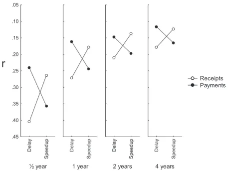
abso-lute magnitude effect, and the delay effect.Figure 2shows the

observed values of r, omitting outcome magnitude. (The values of r are reversely scaled for comparability with subsequent results.) We see the delay–speedup asymmetry, and, consistent withFigure 1, its attenuation for longer delays. We further see the gain–loss asymmetry for all delays, except for 2 years. This is an anomalous result that the tradeoff models will be unable to explain.

Table 1 shows the number of free parameters and the badness-of-fit of the seven models. Because the design of

Benzion et al. (1989) does not include the neutral frame, the time-frame tradeoff model cannot estimate both hypersensitiv-ity to time lost and hyposensitivhypersensitiv-ity to time gained, so that it has one parameter less than the outcome-frame tradeoff model. We estimated hypersensitivity, but we would obtain exactly the same results if we estimated hyposensitivity instead. Going down the list of competing models, badness-of-fit decreases, with the time-frame tradeoff model coming out best.

The outcome-frame and time-frame tradeoff models are the only ones that qualitatively predict the full range of anomalies

in these data. Table 2 shows the parameter estimates upon

estimating these models on the set of n data points. There is

Receipts Payments ½ year S p ee du p De la y .05 .10 .15 .20 .25 .30 .35 .40 .45 1 year S p ee du p De la y 2 years S p ee du p De la y 4 years S p ee du p De la y

r

Figure 2. Benzion et al.’s (1989)indifference data from matching. This figure shows the observed values of r (reversely scaled). We observe the delay–speedup asymmetry and its attenuation for longer delays.

(10)

modest loss aversion (␭), reflecting a modest gain–loss asym-metry in the data. The time-frame tradeoff model exhibits

hypersensitivity to time lost (␬l), and the outcome-frame

tradeoff model exhibits hypersensitivity to worse than expected

states (␮l) and hyposensitivity to better than expected states

(␮g).

The top and bottom panels ofFigure 3show the predictions of the

outcome-frame tradeoff model and the time-frame tradeoff model, respectively. It is clear that the time-frame tradeoff model most closely reproduces the qualitative patterns in the data. Although both models predict the delay–speedup and gain–loss asymmetries, and their attenuation for longer delays, the outcome-frame tradeoff model predicts far too much attenuation, so much so that, at the 4-year delay, it predicts no delay–speedup asymmetry for gains.

Figure 4shows the results for outcome magnitude. The models yield the same predictions, involving progressively smaller de-creases of r as outcome magnitude inde-creases. The result for the $5,000 outcomes, showing a relatively large decrease of r, is anomalous to this prediction, and it suggests that outcomes of this magnitude were qualitatively different for the participants.

More Indifference Data From Matching

In this study, we analyze indifference data from a matching study that includes the neutral frame, so that we can estimate the full time-frame tradeoff model, and evaluate the efficacy of this model and the outcome-frame tradeoff model in predicting the gain–loss asymmetry in both the neutral frame and the delay–speedup frames.

Method

Independent and dependent variables. There were 32 option

pairs resulting from a 2 (outcome matched: xLor xS)⫻ 2 (decision

frame: neutral or delay–speedup) ⫻ 2 (outcome sign: positive or

negative)⫻ 2 (outcome magnitude: €100 or €900) ⫻ 2 (delay to the

larger outcome: 1/2 year or 2 years) factorial design. The first two factors were manipulated between participants, the others within participant, so that each participant matched eight options pairs. For each option pair, we computed the geometric mean of the per-period

discount factor␦ (Equation 4). This practice is to be recommended,

because taking the geometric mean of discount factor␦ is the same as

taking the geometric means of xSand xLand computing␦ from there,

meaning the functional relation between outcomes and discount mea-sures is preserved in the aggregate data. Analyses were performed on

arithmetic means of log(␦). The full breakdown of our results is given

inTable 3.4

Participants. A total of 280 Portuguese residents, 45% male and averaging 33 years of age, participated by completing an on-line questionnaire. Invitations for participating in the investigation were sent out by e-mail to the acquaintances of eight students who had enrolled in a research seminar of the first author. The receivers of this e-mail were urged to invite their acquaintances in turn. Most partic-ipants had an academic degree (84%), and most were employed (59%) or students (34%).

Procedure. Participants filled in the variable outcome that yielded indifference between SS and LL. An item for the delay of

a receipt would read: “You are entitled to receive€100 today, but

you can choose to delay the receipt, and receive more in 2 years.” The participants then filled in the blank in the following statement:

“Instead of receiving€100 today, I agree to delay the receipt if I

receive at a minimum€_____ in 2 years.” In the neutral frame, an

item for the xL matching of a receipt would read: “For me,

receiving€100 today is as good as receiving €_____ in 2 years”

(cf. Takeuchi, 2011).5 _{Similar items were developed for the}

re-4_{Ninety participants discounted an outcome by a greater amount over}

the 1/2 year interval than over the 2 years interval for at least one of the option pairs in the outcome sign ⫻ outcome magnitude subdesign, or discounted the $100 outcome by a greater amount than the $900 outcome for at least one of the option pairs in the outcome sign⫻ delay length subdesign. They were excluded from the analyses. The 68% survival rate (190/280) is comparable to the 72% survival rate (204/282) reported by Benzion et al. (1989), but their criterion was incomplete rather than incorrect responding (but seeShelley, 1993;Thaler, 1981). The survival rates were significantly higher for xLmatching than for xSmatching, .81⫺

.54⫽ .27, ␹2₍₁₎_{⫽ 23.64, p ⫽ .00, which suggests that our participants had}

far less difficulty with present-to-future than with future-to-present con-versions. The exclusion of inconsistent responders may not be innocuous, in that their mental process may not be the same as that of the consistent responders.

5_{Shelley (1993,}_{Figure 2, p. 811) operationalized the neutral frame as}

follows: “You owe a debt of $x in t years to a public institute. What is the (negative) value,⫺$x, of that debt to you now?” Her results suggest that this was understood as a speedup frame instead: Implied discount rates in the “neutral” frame were higher for losses than for gains, just as they were in the speedup frame.

Table 1

Benzion et al.’s (1989)Indifference Data From Matching: Badness-of-Fit Upon Cross-Validating the Discounting Models and the Tradeoff Models on r

Model ka _RMSDb _⫺log(L)c

Exponential discounting model 1 0.10 ⫺54.57

Hyperbolic discounting model 1 0.09 ⫺62.18

Generalized hyperbolic discounting model 2 0.08 ⫺67.94

Outcome-frame discounting model 3 0.07 ⫺75.12

Basic tradeoff model 4 0.07 ⫺80.66

Outcome-frame tradeoff model 6 0.06 ⫺86.90

Time-frame tradeoff model 5 0.04 ⫺108.40

a_{Number of free parameters.} b_{The root-mean-square deviation,}

兹

兺

共yi⫺yˆi⫺i兲2⁄n, where n is the number of data points, yiis the observed value of

dependent variable y for data point i, and yˆi⫺iis the predicted value of y for data point i, obtained by estimating the model on the remaining n⫺ 1 data

points. The standard deviation,

兹

兺

共yi⫺y៮兲2⁄n, where y៮ is the mean value of y, is 0.10. c⫺ log共L兲 ⫽ 0.5n共log共

兺

共yi⫺ yˆi⫺i兲2⁄n兲 ⫹ log共2␲兲 ⫹ 1兲, where

log(L) is the maximum log-likelihood of the estimated model (seeBurnham & Anderson, 2003;Spiess & Neumeyer, 2010).

(11)

maining conditions. In the introduction to the questionnaire, par-ticipants completed a rehearsal trial. Upon completing the exper-imental trials, they provided their demographics.

Results

We conducted a mixed-design analysis of variance (ANOVA)

on log(␦) with three within-participant factors (outcome sign,

outcome magnitude, and delay length) and two

between-participants factors: One factor contrasted xL matching with xS

matching, the other factor contrasted the neutral frame with the delay–speedup frames. Seven main results emerged from this analysis: (1) The delay–speedup and gain–loss asymmetries in the delay–speedup frames and the gain–loss asymmetry in the neutral

frame, F(1, 186)⫽ 21.40, p ⫽ .00, ␩P2 ⫽ .12; (2) the gain–loss

asymmetry across frames, F(1, 186)⫽ 13.66, p ⫽ .00, ␩P2⫽ .07;

(3) a less pronounced gain–loss asymmetry in the delay–speedup

frames than in the neutral frame, F(1, 186)⫽ 4.22, p ⫽ .04, ␩P2⫽

.02; (4) an attenuation of the delay–speedup and gain–loss

asym-metries for longer delays, F(1, 186)⫽ 15.52, p ⫽ .00, ␩_P2⫽ .08;

(5) the absolute magnitude effect, F(1, 186) ⫽ 26.97, p ⫽ .00,

␩P2 ⫽ .14; (6) an attenuation of the absolute magnitude effect for

longer delays, F(1, 186)⫽ 5.62, p ⫽ .02, ␩_P2 ⫽ .03; and (7) the

delay effect, F(1, 186) ⫽ 81.41, p ⫽ .00, ␩P2 ⫽ .44.6 The left

panels ofFigure 5 show the observed values of␦ along a

loga-rithmic scale. In the neutral frame, xSmatching and xLmatching

yielded virtually the same results, so that we collapse across these conditions.

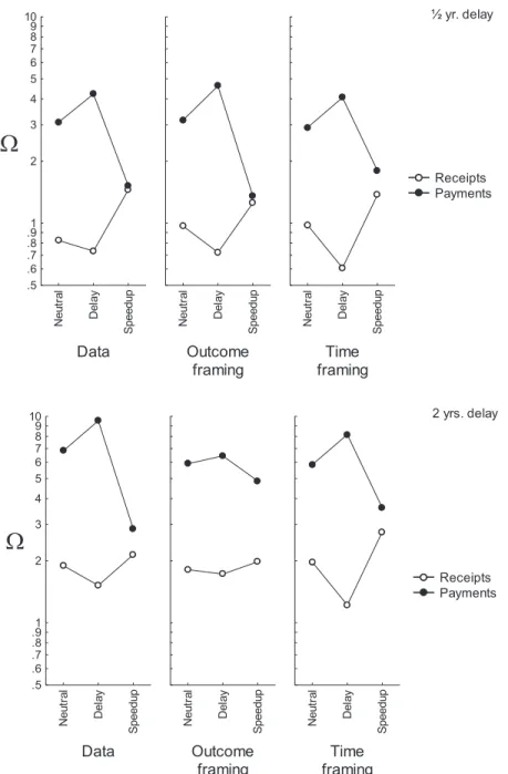
Table 4shows the number of free parameters and the badness-of-fit of the seven models upon n-fold cross-validation on the experimental trials. Going down the list of competing models, badness-of-fit decreases, but with one exception: The outcome-frame discounting model, which fails to predict the gain–loss asymmetry and the absolute magnitude effect, came out better than the basic tradeoff model, which fails to predict the delay–speedup asymmetry, and the outcome-frame tradeoff model, which quali-tatively predicts all anomalies in the data. This suggests that the added complexity of the outcome-frame tradeoff model captured more noise than regularity. The time-frame tradeoff model comes out best from the model contest.

Table 5 shows the parameter estimates upon estimating the outcome-frame and time-frame tradeoff models on the full set of n

data points. Loss aversion (␭) is more pronounced than in the

reanalysis of Benzion et al. (1989). In the time-frame tradeoff

model, hypersensitivity to time lost is more pronounced than

hyposensitivity to time gained, that is, log(␬l) ⫽ 0.65 ⬎ 0.14 ⫽

⫺log(␬g).7In the outcome-frame tradeoff model, however,

hyper-sensitivity to worse than expected states is no more pronounced, and slightly less pronounced, than hyposensitivity to better than

expected states, that is, log(␮l)⫽ 0.05 ⬍ ⫺log(␮g)⫽ 0.06.

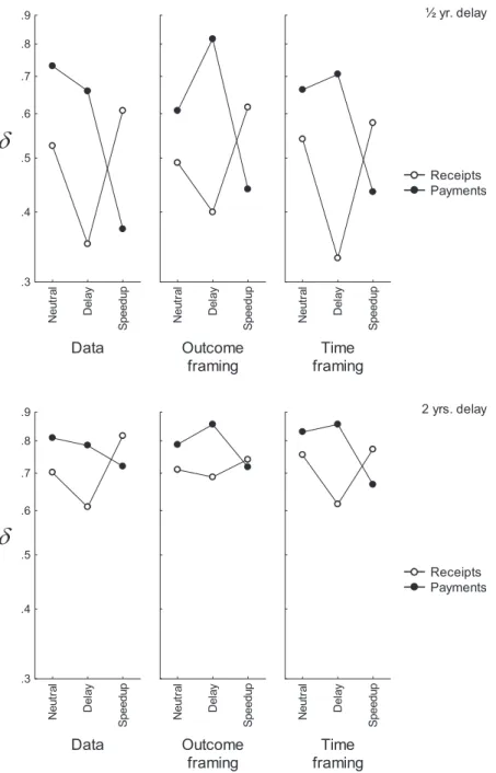
The center panels and right panels ofFigure 5show the

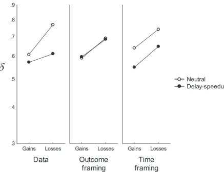
predic-tions of the outcome-frame tradeoff model and time-frame tradeoff model, respectively. In the predictions of both models, the gain– loss asymmetry is as pronounced in the delay–speedup frames as in the neutral frame, whereas, in the data, the gain–loss asymmetry is less pronounced in the delay–speedup frames than in the neutral

frame. This can be seen more easily inFigure 6. It can also be seen

that, across gains and losses, the outcome-frame tradeoff model incorrectly predicts as much discounting in the delay–speedup frames as in the neutral frame, while the time-framing tradeoff model correctly predicts more discounting in the delay–speedup frames than in the neutral frame. Omitted from Figures 5 and 6 is outcome magnitude. Both tradeoff models closely reproduced the absolute magnitude effect and its attenuation for longer delays.

6_{Corollary and secondary results emerged from the ANOVA: (I) More}

discounting in the delay–speedup frames than in the neutral frame, F(1, 186)⫽ 6.01, p ⫽ .02, ␩P

2_{⫽ .03; (II) an attenuation of the difference in} discounting between the delay–speedup frames and the neutral frame for longer delays, F(1, 186)⫽ 10.80, p ⫽ .00, ␩P

2_{⫽ .06; (III) an outcome sign} by outcome matched interaction across decision frames, F(1, 186)⫽ 20.37, p⫽ .00, ␩P

2 _{⫽ .11 (a corollary of Result 1); (IV) an attenuation of the} outcome sign by outcome matched interaction for longer delays, F(1, 186)⫽ 13.00, p ⫽ .00, ␩P

2_{⫽ .07 (a corollary of Result 4); (V) an outcome} sign by outcome magnitude interaction, in that the gain–loss asymmetry was more pronounced for small outcomes than for large ones, F(1, 186)⫽ 7.74, p ⫽ .01, ␩2P ⫽ .04 (see Loewenstein & Prelec, 1992); (VI) an

attenuation of the outcome sign by outcome magnitude interaction for longer delays, F(1, 186)⫽ 4.12, p ⫽ .04, ␩P2 ⫽ .02; (VII) an outcome

magnitude by outcome matched interaction, in that the absolute magnitude effect was more pronounced when the later outcome was matched than when the sooner outcome was matched, F(1, 186)⫽ 17.16, p ⫽ .00, ␩P

2_⫽ .09; and (VIII) an attenuation of the outcome magnitude by outcome matched interaction for longer delays, F(1, 186)⫽ 7.70, p ⫽ .01, ␩P

2_{⫽ .04.}

7_Because_␬

l ⬎ 1 and 0 ⬍ ␬g⬍ 1, we must compare log(␬l) with

⫺log(␬g).

Table 2

Benzion et al.’s (1989)Indifference Data From Matching: Parameter Estimates and Statistical Tests Upon Estimating the Tradeoff Models on r

Outcome framing Time framing

Parameter Estimate t(58)a _p _Parameter _Estimate _t(59)a _p

␬ 7.53 6.06 .00 _␬ 6.39 7.93 .00 ␬l 1.45 7.25 .00 ␶ 1.75 3.68 .00 ␶ 1.77 4.91 .00 ␥ 0.04 6.54 .00 ␥ 0.04 8.84 .00 ␭ 1.07 1.31 .10 ␭ 1.13 2.88 .00 ␮l 1.01 3.87 .00 ␮g 0.99 ⫺3.25 .00

Note. The models were estimated on 64 data points (seeBenzion et al., 1989,Table 1).

a_{Testing whether}_{␬, ␶, and ␥ are reliably greater than zero, whether ␬}

l,␭, and ␮lare reliably greater than one, and whether␮gis reliably smaller than one.

(12)

It is possible to run an additional cross-validation check, be-cause, in the introduction to the questionnaire, the participants

performed a rehearsal trial involving a medium-large gain (€300,

the geometric mean of €100 and €900) over a medium-length

interval (1 year, the geometric mean of 1/2 year and 2 years), and this trial can be used for cross-validation. For each model, we used the parameters estimated from the 32 experimental trials to predict

log(␦) in the four different rehearsal trials corresponding to the

four cells in the 2 (outcome matched) ⫻ 2 (decision frame)

between-participants subdesign. This subdesign only includes the delay–speedup asymmetry, and none of the remaining anomalies

(i.e., the gain–loss asymmetry, the absolute magnitude effect, the delay effect, and the attenuation of the delay–speedup asymmetry

for longer delays). The results are shown inTable 4, under the

heading “rehearsal trial.” Among the models that fail to predict the delay–speedup asymmetry, the basic tradeoff model came out worse than the three discounting models (exponential, hyperbolic, and generalized hyperbolic), and, among these discounting mod-els, the generalized hyperbolic discounting model came out worse than the two discounting models it includes as special cases (exponential and hyperbolic), suggesting that the added complex-ity may be a handicap in the extrapolation to stimuli with different

Receipts Payments ½ year S p ee du p De la y .05 .10 .15 .20 .25 .30 .35 .40 .45 1 year S p ee du p De la y 2 years Sp e e d u p De la y 4 years S p ee du p De la y

r

Receipts Payments ½ year S p ee du p De la y .05 .10 .15 .20 .25 .30 .35 .40 .45 1 year S p ee du p De la y 2 years S p ee du p De la y 4 years S p ee du p De la y

r

Figure 3. Benzion et al.’s (1989)indifference data from matching. This figure shows the predicted values of r from the outcome-frame tradeoff model (top panel) and the time-frame tradeoff model (bottom panel).

(13)

characteristics (i.e., a constant rather than a varying outcome sign, a different and constant outcome magnitude, and a different and constant delay length). Again, the outcome-frame tradeoff model came out worse than the outcome-frame discounting model, which, in turn, came out worse than the time-frame tradeoff model, the winner in this additional cross-validation check.

Discussion

Among the models that predict the delay–speedup asymmetry, the time-frame tradeoff model came out better than the

outcome-frame tradeoff model and the outcome-outcome-frame discounting model,

consistent with our reanalysis of the data from Benzion et al.

(1989). However, outcome-frame tradeoff model came out slightly worse than the outcome-frame discounting model, when the for-mer is more comprehensive than the latter. This suggests that the added complexity of the outcome-frame tradeoff model captured more noise than regularity, even though it captured the gain–loss asymmetry and the absolute magnitude effect, whereas the outcome-frame discounting model did not. Actually, our own matching data may have been noisier than Benzion et al.’s data,

Table 3

Indifference Data From Matching: Delays, Outcomes, and Per-Period Discount Factors

Neutral framea _{Delay–speedup frames}b

tL c _x S d _x L d _␦e _t L c _x S d _x L d _␦e ½ 100 159.45 .393 ½ 100 204.08 .240 2 100 264.27 .615 2 100 364.67 .524 ½ 900 1,054.51 .728 ½ 900 1256.70 .513 2 900 1,434.68 .792 2 900 ⫺1,798.23 .707 ½ ⫺100 ⫺122.63 .665 ½ ⫺100 ⫺140.43 .507 2 ⫺100 ⫺185.96 .733 2 ⫺100 ⫺202.73 .702 ½ ⫺900 ⫺999.60 .811 ½ ⫺900 ⫺972.14 .857 2 ⫺900 ⫺1,134.70 .891 2 ⫺900 ⫺1,172.60 .876 ½ 70.39 100 .496 ½ 74.44 100 .554 2 44.94 100 .670 2 61.27 100 .783 ½ 659.72 900 .537 ½ 735.40 900 .668 2 493.62 900 .741 2 653.14 900 .852 ½ ⫺86.23 ⫺100 .744 ½ ⫺62.47 ⫺100 .390 2 ⫺61.53 ⫺100 .784 2 ⫺53.56 ⫺100 .732 ½ ⫺757.91 ⫺900 .709 ½ ⫺536.97 ⫺900 .356 2 ⫺629.56 ⫺900 .836 2 ⫺452.68 ⫺900 .709 a_N_{⫽ 61 (x}

Lmatching) and N⫽ 46 (xSmatching). bN⫽ 53 (delay frame) and N ⫽ 30 (speedup frame). cDelays in years. dOutcomes in euros.

Geometric means. e_{Geometric means.}

Data $4 0 $2 00 $1 ,0 00 $5 ,0 00 .05 .10 .15 .20 .25 .30 .35 .40 .45 Outcome framing $4 0 $2 00 $1 ,0 00 $5 ,0 00 Time framing $4 0 $2 00 $1 ,0 00 $5 ,0 00

r

Figure 4. Benzion et al.’s (1989) indifference data from matching. Observed and predicted values of r (reversely scaled). Predictions from the tradeoff models. We observe the absolute magnitude effect for $200, its attenuation for $1,000, and its accentuation for $5,000.