UNIVERSIDADE DE LISBOA FACULDADE DE CIÊNCIAS
Models for multi-depot routing problems
“ Documento Definitivo”
Doutoramento em Estatística e Investigação Operacional Especialidade de Otimização
Daniel Rebelo dos Santos
Tese orientada por:
Professor Doutor Luís Eduardo Neves Gouveia
UNIVERSIDADE DE LISBOA FACULDADE DE CIÊNCIAS
Models for multi-depot routing problems
Doutoramento em Estatística e Investigação Operacional Especialidade de Otimização
Daniel Rebelo dos Santos
Tese orientada por:
Professor Doutor Luís Eduardo Neves Gouveia Júri:
Presidente:
● Doutora Maria Eugénia Vasconcelos Captivo, Professora Catedrática, Faculdade de Ciências da Universidade de Lisboa
Vogais:
● Doutor Agostinho Miguel Mendes Agra, Professor Auxiliar, Departamento de Matemática da Universidade de Aveiro
● Doutor José Manuel Vasconcelos Valério de Carvalho, Professor Catedrático, Escola de Engenharia da Universidade do Minho
● Doutor José Manuel Pinto Paixão, Professor Catedrático, Faculdade de Ciências da Universidade de Lisboa ● Doutor Luís Eduardo Neves Gouveia, Professor Catedrático, Faculdade de Ciências da Universidade de Lisboa (Orientador)
● Doutora Maria Eugénia Vasconcelos Captivo, Professora Catedrática, Faculdade de Ciências da Universidade de Lisboa
Documento especialmente elaborado para a obtenção do grau de doutor
Esta dissertação foi financiada pela Universidade de Lisboa ao abrigo do Programa de Bolsas de Doutoramento da Universidade de Lisboa
Agradecimentos
Em primeiro lugar queria agradecer à Raquel. Tudo o que faço, incluindo esta dissertação, é-lhe totalmente dedicado. Eu não seria a mesma pessoa e o meu percurso académico até este nível não teria existido se nunca tivesse tido o privilégio de a conhecer e de ser seu companheiro. O trabalho que aqui deixo foi grande parte fruto da sua paciência para me ouvir, para conversar comigo e, em especial na fase final, para me garantir as condições de trabalho ideais. Eu sei que achará que estou a exagerar, mas ambos sabemos que no fundo, e objetivamente, a Raquel terá não uma, mas duas dissertações de doutoramento de sua autoria, a sua e a minha.
Queria prestar um agradecimento muito especial e sentido ao meu orientador, o Professor Doutor Luís Eduardo Neves Gouveia, pela sua disponibilidade e entrega a esta dissertação a 100% e pelo vasto conhecimento que me passou. Foi, mais uma vez, uma grande honra ser orientado por um dos melhores do mundo na sua área que, apesar disso, sempre me tratou como se fôssemos normais colegas de trabalho. Olharei para todos os momentos passados no seu gabinete a escrever no quadro branco com grande saudade.
Gostaria de agradecer à minha mãe, Elvira, pelo seu apoio incondicional em todas as decisões que tomei, que tomo e que tomarei, e pela educação pessoal e académica que me proporcionou. Ter a certeza que em qualquer situação poderei sempre recorrer a ela é fundamental para mim. Agradeço também ao senhor Joaquim, pai da Raquel, por, apesar de não ser sua obrigação, assegurar constantemente o meu bem-estar. Um obrigado também à Maria Fernanda, avó da Raquel, e ao senhor Júlio, avô da Raquel, por me permitirem recorrer à sua ajuda sem nunca me rejeitarem nada.
I would like to thank Mario Ruthmair, for his availability in teaching me all the computational tools which I required for this dissertation and for never rejecting to help me in any situation, and Tolga Bektaş, for indirectly teaching me many amusing English expressions and for his important contribution to the work developed in this dissertation. Quero ainda agradecer a todos os meus professores, em especial àqueles que me permitiram participar em várias conferências que muito contribuíram para a minha evolução. Gostaria também de agradecer ao Michele, meu colega de gabinete durante grande parte desta dissertação, pela sua ajuda e pela sua companhia. Grazie mille, Michele.
por me proporcionar as condições justas para que pudesse terminar a dissertação, e à Universi-dade de Lisboa, por financiar esta dissertação ao abrigo do Programa de Bolsas de Doutoramento da Universidade de Lisboa.
Finalmente, a todos os que de uma forma ou outra contribuíram para esta dissertação, nem que tenha sido apenas por me ouvirem ou por se mostrarem interessados no meu trabalho, o meu obrigado.
Abstract
In this dissertation we study two problems. In the first part of the dissertation we study the multi-depot routing problem. In the multi-depot routing problem we are given a set of depots and a set of clients and the objective is to find a set of routes with minimum total cost, one for each depot, such that each route starts and ends at the same depot and all clients are visited in one and only one route. The requirement that routes must start and end at the same depot is modeled by so-called path elimination constraints. We present a formulation which includes a newly developed set of multi-cut path elimination constraints and a branch-and-cut algorithm based on the new formulation that it is able to solve both asymmetric and symmetric instances with up to 300 clients and 60 depots. Additionally, we present other approaches to model path elimination constraints, including a formulation which provides linear programming relaxation values which are close to the optimal value in the instances tested.
In the second part of the dissertation we study the Hamiltonian p-median problem. In the Hamiltonian p-median we are given a set of nodes and the objective is to find p circuits with minimum total cost such that each node is in one and only circuit. We propose a formulation based on the concept of acting depot which attributes the role of artificial depot to p of the nodes. This formulation is a non-straightforward adaptation of the new model proposed for the multi-depot routing problem and it is based on a novel idea in which the standard arc variables are split into three cases depending on whether none or exactly one of its endpoints is an acting depot. We present a branch-and-cut algorithm based on the new formulation which is able to solve asymmetric instances with up to 171 nodes and symmetric instances with up to 100 nodes.
Keywords: multi-depot routing, Hamiltonian p-median, integer linear programming,
Resumo
Nesta dissertação estudamos dois problemas de otimização. Na primeira parte da dissertação abordamos o multi-depot routing problem. Dado um grafo cujos nodos são particionados num conjunto de depósitos e num conjunto de clientes, o objetivo do multi-depot routing problem é encontrar um conjunto de rotas, uma para cada depósito, tais que: (i) cada cliente é visitado numa e numa só rota; (ii) cada rota começa e termina no mesmo depósito; e (iii) o custo das rotas é o menor possível. Consideramos que o custo de uma rota é a soma dos custos dos arcos utilizados, sendo que nesta dissertação permitimos custos assimétricos, isto é, o custo de ir de A para B pode não ser o mesmo de ir de B para A. Assim sendo, os modelos que apresentamos são baseados em grafos orientados.
A condição (ii) de que cada rota tem de começar e terminar no mesmo depósito é geral-mente modelada com recurso a restrições que na literatura se designam por path elimination
constraints. Estas restrições garantem que qualquer caminho que ligue dois depósitos não é
admissível. Nesta dissertação propomos uma formulação baseada num novo conjunto de path
elimination constraints que podem ser vistas como restrições de corte num grafo com três níveis.
Além do nível dos clientes, o grafo com três níveis tem um nível para os depósitos e outro para uma cópia de cada depósito, sendo que os arcos que entram no depósito no grafo original, entram na sua cópia no grafo com três níveis. As novas restrições resultam da projeção no espaço das usuais variáveis associadas a cada arco de um sistema de fluxos definido no grafo com três níveis que garante que uma unidade de fluxo é enviada de cada depósito para a sua cópia. Esta relação deriva do teorema de fluxo máximo/corte de capacidade mínima o que nos permite desenvolver um algoritmo de separação exato e eficiente para as novas restrições.
Com base na nova formulação apresentamos um algoritmo de branch-and-cut que faz uso da separação eficiente das novas path elimination constraints para resolver instâncias, tanto com custos assimétricos como com custos simétricos, com até 300 clientes e até 60 depósitos. O algorithm de branch-and-cut foi implementado em C++ e utiliza a framework do CPLEX que é um software que permite a resolução de problemas de otimização com base em modelos para problemas de programação inteira. O algoritmo de branch-and-cut incorpora técnicas para garantir a sua eficiência, como a limitação do número de desigualdades violadas adicionadas em cada iteração do algoritmo de planos de corte e a utilização de uma heurística simples, mas
eficaz, que produz soluções admissíveis com base na relaxação linear em cada nodo da árvore de pesquisa.
Nesta dissertação apresentamos também outras abordagens para modelar a restrição de que cada rota tem de começar e terminar no mesmo depósito. Alguns dos modelos apresentados têm por base um conjunto de variáveis que indicam se um dado cliente está ou não no circuito de um dado depósito. Com base em igualdades simples é possível mostrar que estas variáveis estão associadas às variáveis de fluxo do sistema de fluxos definido no grafo com três níveis, logo, é possível estabelecer uma comparação com os modelos apresentados anteriormente, em particular as novas path elimination constraints propostas. Apresentamos ainda outro modelo baseado em dois sistemas de fluxo, um que garante que uma unidade de fluxo é enviada de cada depósito para cada cliente que esteja no seu circuito e outro que garante o contrário, de tal forma que, em conjunto, é garantida a existência de um circuito para cada depósito. Mostramos também que estes dois sistemas de fluxo podem ser relacionados com o sistema de fluxos do grafo com três níveis e, recorrendo a técnicas de projeção, mostramos que é possível definir um modelo equivalente que não necessita dos sistemas de fluxo duplos e que é mais fácil de utilizar na prática. Por fim, apresentamos um conjunto de resultados computacionais para avaliar a qualidade dos valores da relaxação linear dos vários modelos apresentados e, em particular, mostramos que o modelo que resulta dos sistemas de fluxo duplos é um modelo cujo valor da relaxação linear está perto do valor ótimo nas instâncias testadas.
Na segunda parte da dissertação estudamos o Hamiltonian p-median problem. Para este problema é-nos dado um grafo (que mais uma vez assumimos orientado) e uma função de custo associada aos arcos do grafo. O objetivo do Hamiltonian p-median problem é encontrar p cir-cuitos tais que: (i) cada nodo do grafo está num e num só circuito; e (ii) o custo dos p circir-cuitos é o menor possível. Começamos por apresentar um modelo genérico para o problema que é baseado no conceito de depósito artificial, isto é, p dos nodos do grafo são escolhidos para atu-arem como um depósito artificial e, por conseguinte, os restantes nodos são clientes artificiais. Com base neste conceito estabelecemos a ligação ao multi-depot routing problem e apresenta-mos um novo modelo que é uma adaptação do modelo baseado nas novas restrições de corte associadas ao grafo de três níveis. Contudo, observamos que este modelo possui duas desvan-tagens. Em primeiro lugar, não cremos que exista um algoritmo de separação eficiente para as restrições de corte associadas ao grafo de três níveis adaptadas para o contexto do Hamiltonian
p-median problem. Em segundo lugar, a utilização do conceito de depósito artificial introduz
problemas de simetria dado que um circuito pode ser representado de forma equivalente tantas vezes quanto o número de nodos que o compõem. Neste modelo não é possível resolver este problema de forma intuitiva.
Assim, apresentamos um novo modelo para o Hamiltonian p-median problem baseado na ideia de dividir as variáveis associadas aos arcos em três conjuntos distintos consoante nenhum
dos seus extremos ou exatamente um dos seus extremos é um depósito artificial. A nova formu-lação permite-nos na mesma adaptar (de forma não trivial) os modelos propostos para o
multi-depot routing problem e, mais importantemente, colmatar as duas desvantagens do primeiro
modelo proposto. Mais concretamente, é possível definir um conjunto de restrições semelhantes às restrições de corte associadas ao grafo de três níveis apresentadas para o multi-depot routing
problem de tal forma que: (i) a sua separação pode ser feita em tempo polinomial; e (ii)
po-dem ser adaptadas para lidar com os problemas de simetria inerentes à utilização do conceito de depósito artificial.
Para terminar, apresentamos um segundo algoritmo de branch-and-cut, desta feita para o
Hamiltonian p-median problem, que utiliza o mesmo tipo de técnicas que o apresentado para o multi-depot routing problem. Este algoritmo de branch-and-cut permite resolver instâncias com
custos assimétricos com até 171 nodos e de instâncias simétricas com até 100 nodos. Fazemos ainda uma comparação com um terceiro algoritmo de branch-and-cut baseado na adaptação de uma formulação da literatura. Os resultados mostram que o algoritmo de branch-and-cut baseado na nova formulação é bastante mais eficiente, em média, do que este terceiro algoritmo. Por fim, mostramos ainda um conjunto de resultados que permitem comparar a nossa abordagem com abordagens da literatura que resolvem uma variante do Hamiltonian p-median problem em que circuitos com apenas dois nodos não são permitidos.
Palavras-chave: rotas com múltiplos depósitos, p-mediana Hamiltoniana, programação linear
Contents
Introduction
1
I
The multi-depot routing problem
3
1 Introducing the multi-depot routing problem 5
1.1 Introduction . . . 5
1.2 Definitions and notation . . . 8
1.3 A generic model . . . 9
2 A new formulation for the multi-depot routing problem 11 2.1 Introduction . . . 12
2.2 Subtour elimination constraints . . . 12
2.3 Path elimination constraints based on arc-depot assignment variables . . . 13
2.3.1 A base model in the space of the x and the z variables . . . . 14
2.3.2 A network flow interpretation of the base model . . . 15
2.3.3 Strengthening the base model . . . 16
2.3.4 A property of the systems of inequalities based on the z variables for symmetric cost instances . . . 19
2.4 A new set of path elimination constraints in the space of the x variables . . . . 20
2.4.1 The multi-cut constraints . . . 20
2.4.2 Establishing a relationship between the multi-cut constraints and the systems of inequalities based on the z variables . . . . 21
2.4.3 A generalization of the multi-cut constraints . . . 22
2.5 Path elimination constraints from the literature . . . 25
2.5.1 An adaptation of the chain-barring constraints . . . 25
2.5.2 A comparison to the multi-cut constraints . . . 27
2.6 Problem variants . . . 29
3 A branch-and-cut algorithm 33
3.1 Introduction . . . 34
3.2 A modern branch-and-cut algorithm . . . 36
3.2.1 Heuristic callback . . . 37
3.2.2 Lazy constraint callback . . . 37
3.2.3 User cut callback . . . 38
3.3 Separation algorithms . . . 38
3.3.1 Separation of the subtour elimination constraints (2.2) . . . 40
3.3.2 Separation of the 1-MCC inequalities (2.13) . . . 41
3.3.3 Separation of the k-MCC inequalities (2.14) . . . 43
3.3.4 Separation of the directed chain-barring constraints (2.17)–(2.18) . . . 44
3.4 Test instances and software/hardware configurations . . . 46
3.5 Preliminary computational experiment . . . 48
3.5.1 Comparing the directed chain-barring constraints to the multi-cut con-straints . . . 48
3.5.2 Evaluating the effectiveness of using valid inequalities . . . 51
3.6 The outline of the branch-and-cut algorithm . . . 53
3.6.1 The underlying formulation . . . 53
3.6.2 Parameters for lazy constraint/user cut callback functions . . . 54
3.6.3 A primal heuristic . . . 55
3.6.4 Symmetry-breaking constraints for symmetric instances . . . 56
3.7 Computational experiment . . . 57
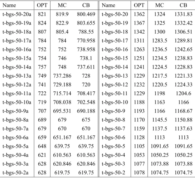
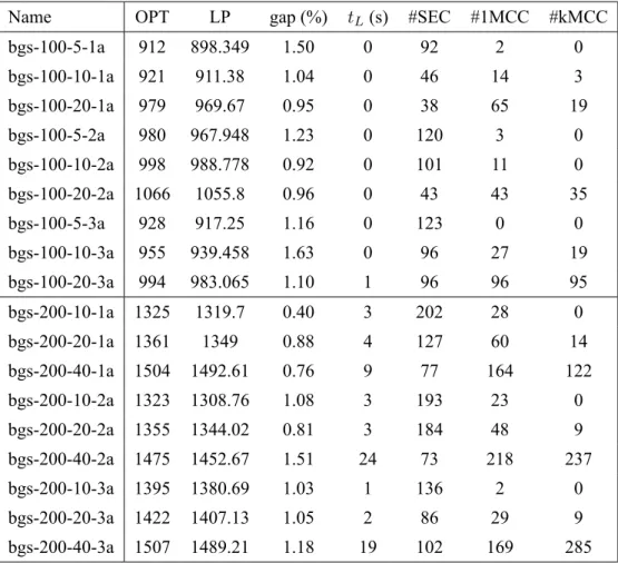
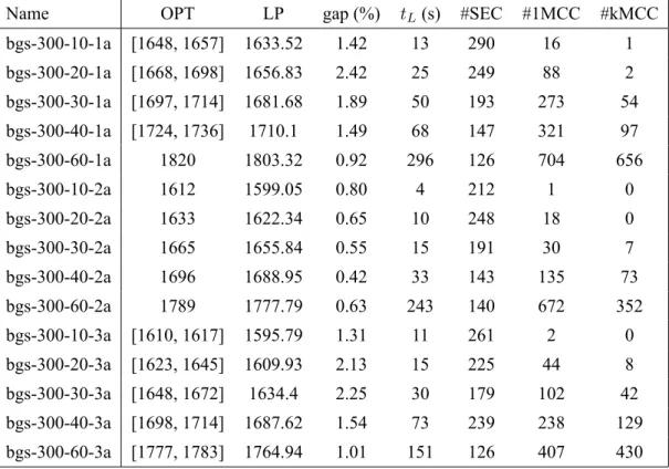
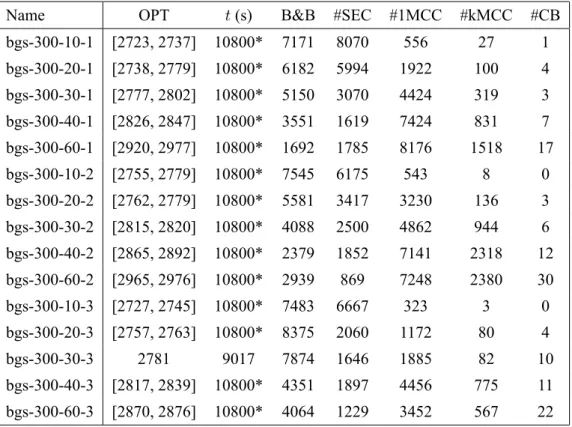
3.7.1 Results for asymmetric instances . . . 57
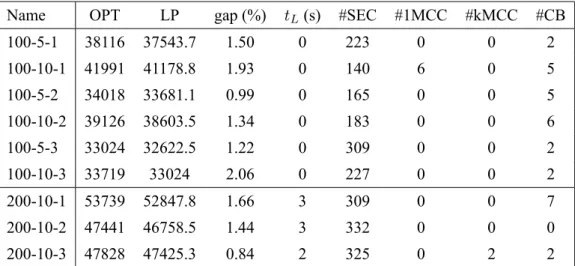
3.7.2 Results for symmetric instances . . . 61
3.7.3 Evaluating the effectiveness of the generalized multi-cut constraints . . 65
3.8 Concluding remarks . . . 68
4 Formulations using depot assignment variables 73 4.1 Introduction . . . 74
4.2 Path elimination constraints based on client-depot assignment variables . . . . 76
4.2.1 A base model in the space of the x and the v variables . . . . 77
4.2.2 Strengthening the base model . . . 79
4.2.3 Generalizations based on arc subsets . . . 80
4.2.4 Generalizations based on depot subsets . . . 80
4.2.5 Generalizations based on arc subsets and depot subsets . . . 81
4.2.6 Exploring the relationship between the v and the z variables in order to strengthen the base model . . . 83
4.2.7 Generalizations based on client subsets . . . 86 xiv
4.2.8 Summary . . . 87
4.2.9 Deriving inequalities in the space of the x variables . . . . 90
4.3 A formulation in the space of the x, the v and the z variables . . . . 92
4.3.1 Path elimination constraints based on double multi-commodity network flow systems . . . 93
4.3.2 Combining the systems of inequalities based on the z variables with the f and g flow systems . . . . 95
4.3.3 Eliminating the f and g flow systems by using the max-flow/min-cut theorem . . . 97
4.3.4 Deriving inequalities in the space of the x and the v variables . . . 100
4.4 Separation algorithms . . . 102
4.4.1 Separation of constraints (4.10), (4.12) and (4.15) . . . 102
4.4.2 Separation of constraints (4.11) . . . 103
4.4.3 Separation of constraints (4.43) . . . 105
4.4.4 Separation of constraints (4.19) . . . 105
4.5 Computational experiment . . . 106
4.5.1 Comparing path elimination constraints in the space of the x and the v variables . . . 107
4.5.2 Comparing formulations using depot assignment variables . . . 110
4.6 Concluding remarks . . . 113
II
The Hamiltonian p-median problem
115
5 Introducing the Hamiltonian p-median problem 117 5.1 Introduction . . . 1175.2 Definitions and notation . . . 120
5.3 A generic model in the space of the arc variables . . . 121
5.4 A model in the space of the arc and of the acting depot variables . . . 122
5.4.1 Modeling the (≤ p) constraints in the space of the x and the y variables 123 5.4.2 Modeling the (≥ p) constraints in the space of the x and the y variables 123 5.4.3 The complete model . . . 125
6 The PQR formulation 127 6.1 Introduction . . . 127
6.2 A formulation in the space of the p, q and r variables . . . 128
6.2.1 Modeling the (≤ p) constraints . . . 130
6.3 Theoretical investigations on the PQR formulation . . . 133
6.3.1 A compact representation of the (≥ p) constraints . . . 134
6.3.2 Breaking symmetries in the PQR formulation . . . 136
6.3.3 Theoretical comparison of the PQR formulation to the model defined in the space of the x and the y variables . . . 139
6.3.4 Generalizations of the multi-cut constraints . . . 141
6.4 An alternative formulation . . . 142
6.4.1 The x-v formulation . . . 143
6.4.2 A comparison of the (≥ p) constraints of the x-v formulation and the PQR formulation . . . 145
6.4.3 A comparison of the (≤ p) constraints of the x-v formulation and the PQR formulation . . . 147
6.5 Concluding remarks . . . 149
7 A branch-and-cut algorithm 151 7.1 Introduction . . . 152
7.2 Separation algorithms . . . 152
7.2.1 Separation of the (≤ p) constraints of the PQR formulation . . . 152
7.2.2 Separation of the (≥ p) constraints of the PQR formulation . . . 154
7.3 Test instances and software/hardware configurations . . . 155
7.4 The outline of the branch-and-cut algorithm . . . 156
7.4.1 Parameters for lazy constraint/user cut callback functions . . . 156
7.4.2 A primal heuristic . . . 157
7.5 Preliminary computational experiments . . . 158
7.5.1 Evaluating the effectiveness of using the lifted (≤ p) constraints . . . . 158
7.5.2 Evaluating the effectiveness of using symmetry-breaking constraints . . 160
7.6 Computational experiment . . . 162
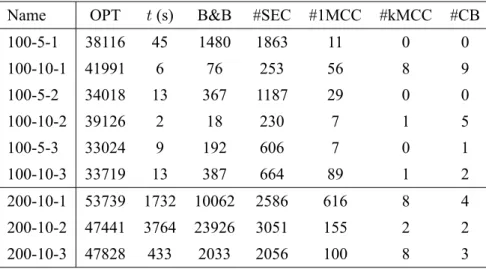
7.6.1 Results for asymmetric instances . . . 162
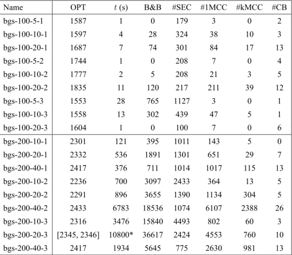
7.6.2 Results for symmetric instances . . . 166
7.7 Additional computational results . . . 170
7.7.1 Numerical comparison between the x-v formulation and the PQR for-mulation . . . 171
7.7.2 Results for the variant in which two-node circuits are not allowed . . . 175
7.8 Concluding remarks . . . 181 xvi
Conclusion
183
A Additional results - Hamiltonian p-median problem 191
A.1 Results for asymmetric instances . . . 192 A.2 Results for symmetric instances . . . 195 A.3 Numerical comparison between the x-v formulation and the PQR formulation . 201 A.4 Results for the variant in which two-node circuits are not allowed . . . 206
List of Figures
1.1 An example of a feasible solution of a multi-depot routing problem . . . 9
2.1 An example of the 3-layered graph . . . 15
3.1 An example of the st-extended graph . . . . 40
3.2 An example of the st-extended 3-layered graph . . . . 40
4.1 Summary of the systems of inequalities presented in Section 4.2 . . . 88
List of Tables
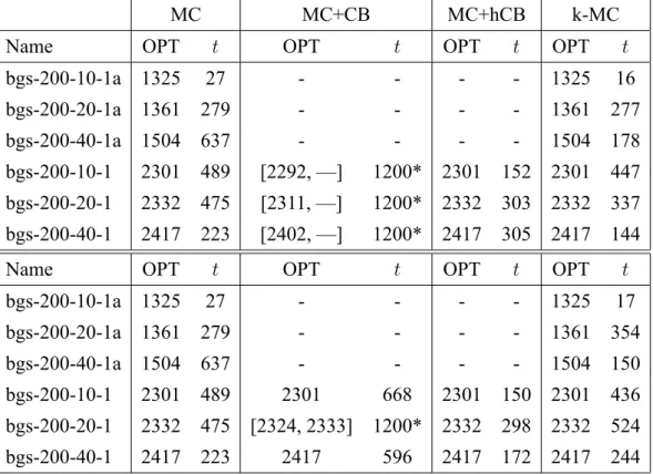
3.1 Comparing the linear programming relaxation values of the MC and the CB formulations . . . 50 3.2 Comparing the solution times of the MC, the MC+CB, the MC+hCB and the
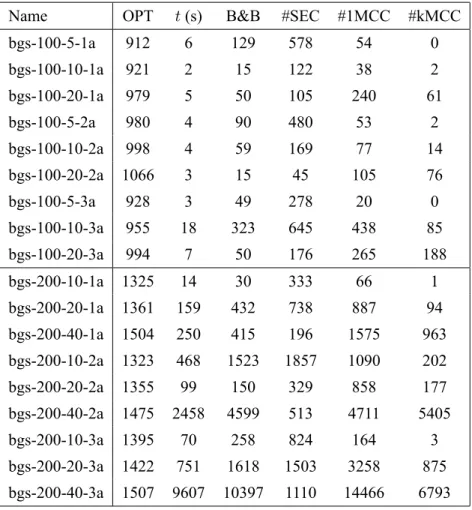
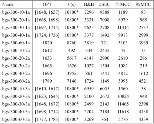
k-MC formulations . . . 52 3.3 Optimal solution results for asymmetric instances (1 of 2) . . . 58 3.4 Optimal solution results for asymmetric instances (2 of 2) . . . 59 3.5 Linear programming relaxation results for asymmetric instances (1 of 2) . . . . 60 3.6 Linear programming relaxation results for asymmetric instances (2 of 2) . . . . 61 3.7 Optimal solution results for symmetric instances (1 of 3) . . . 62 3.8 Optimal solution results for symmetric instances (2 of 3) . . . 63 3.9 Optimal solution results for symmetric instances (3 of 3) . . . 64 3.10 Linear programming relaxation results for symmetric instances (1 of 3) . . . . 65 3.11 Linear programming relaxation results for symmetric instances (2 of 3) . . . . 66 3.12 Linear programming relaxation results for symmetric instances (3 of 3) . . . . 67 3.13 Evaluating the effectiveness of the generalized multi-cut constraints . . . 68 4.1 Comparing the linear programming relaxation values of several path elimination
constraints based on the v variables for asymmetric instances . . . 108 4.2 Comparing the linear programming relaxation values of several path elimination
constraints based on the v variables for symmetric instances . . . 109 4.3 Comparing the linear programming relaxation values of formulations based on
the v variables and formulations based on the z variables for asymmetric instances 111 4.4 Comparing the linear programming relaxation values of formulations based on
the v variables and formulations based on the z variables for symmetric instances 112 7.1 Comparison the solution times of different (≤ p) constraints . . . 159 7.2 Evaluating the effectiveness of using symmetry-breaking constraints of type I
(1 of 2) . . . 161 7.3 Evaluating the effectiveness of using symmetry-breaking constraints of type I
7.4 Optimal solution results for asymmetric instances (1 of 2) . . . 163 7.5 Optimal solution results for asymmetric instances (2 of 2) . . . 164 7.6 Linear programming relaxation results for asymmetric instances (1 of 2) . . . . 165 7.7 Linear programming relaxation results for asymmetric instances (2 of 2) . . . . 166 7.8 Optimal solution results for symmetric instances (1 of 2) . . . 167 7.9 Optimal solution results for symmetric instances (2 of 2) . . . 168 7.10 Linear programming relaxation results for symmetric instances (1 of 2) . . . . 169 7.11 Linear programming relaxation results for symmetric instances (2 of 2) . . . . 170 7.12 Numerical comparison between the x-v and the PQR formulations (1 of 2) . . . 173 7.13 Numerical comparison between the x-v and the PQR formulations (2 of 2) . . . 174 7.14 Evaluating the effectiveness of the non-trivial two-node circuit elimination
con-straints . . . 176 7.15 Optimal solution results for symmetric instances (two-node circuits not allowed)
(1 of 2) . . . 177 7.16 Optimal solution results for symmetric instances (two-node circuits not allowed)
(2 of 2) . . . 178 7.17 Linear programming relaxation results for symmetric instances (two-node
cir-cuits not allowed) (1 of 2) . . . 179 7.18 Linear programming relaxation results for symmetric instances (two-node
cir-cuits not allowed) (2 of 2) . . . 180 A.1 Optimal solution results for asymmetric instances (appendix) . . . 192 A.2 Linear programming relaxation results for asymmetric instances (appendix) . . 193 A.3 Optimal results for symmetric instances (appendix) . . . 195 A.4 Linear programming relaxation results for symmetric instances (appendix) . . . 197 A.5 Numerical comparison between the x-v and the PQR formulations (appendix) . 201 A.6 Optimal solution results for symmetric instances (two-node circuits not allowed)
(appendix) . . . 206 A.7 Linear programming relaxation results for symmetric instances (two-node
cir-cuits not allowed) (appendix) . . . 207
Introduction
The field of Operations Research is a thriving mathematics discipline with the main purpose of proposing solution methods for optimization problems. One of the most important and widely studied type of problems are routing problems. Routing problems usually stem from the area of distribution logistics where one wishes to find a set of routes that visit given locations while simultaneously minimizing some objective (e.g., operational costs). Often a route starts and ends at a specific location denoted by depot and some companies may have several depots from where their distribution vehicles depart.
In this dissertation we study routing problems in which there exists more than one depot or, in other words, multi-depot routing problems. The dissertation is divided into two parts, each one corresponding to a different optimization problem. In the first part of the dissertation we study the multi-depot routing problem. In this optimization problem we are given a set of depots and a set of locations that need to be visited. The objective is to find a set of routes, one for each depot, such that: (i) each location is visited in one and only one route; (ii) each route starts and ends at the same depot; and (iii) a given cost function is minimized. In the second part of the dissertation we study the Hamiltonian p-median problem where, given a set of locations, we must find p circuits such that: (i) each location is in one and only one circuit; and (ii) a given cost function is minimized. Albeit different problems, we show in this dissertation that the multi-depot routing problem can be seen as a particular case of the Hamiltonian p-median problem.
We strongly believe that the additional condition in multi-depot routing problems that routes must start and end at the same depot has not been given sufficient attention in the literature. Ad-ditionally, we believe that the Hamiltonian p-median is lacking recent algorithmic development given that most works in the literature address a variant of the problem. These two points justify the work developed within the scope of this Ph.D. dissertation.
This dissertation has three distinct aims. The first aim is to present a number of different mathematical models for the multi-depot routing problem focusing, in particular, on modeling the restriction that routes must start and end at the same depot. The second aim is to provide an efficient solution method which can provide good quality (hopefully, the best possible) solutions for the multi-depot routing problem based on the theoretical models proposed. The third and
INTRODUCTION
final aim is to establish a link between the multi-depot routing problem and the Hamiltonian p-median problem which allows us to (not necessarily in a straightforward way) adapt both the models and the solution methods proposed for the former to the latter.
This dissertation is organized in the following way. Part I is divided into four chapters. In Chapter 1 we formally introduce the multi-depot routing problem. In particular, we present notation used throughout the first part of the dissertation and a generic model for the problem. In Chapter 2 we propose a model for the multi-depot routing problem which includes newly developed constraints that guarantee that each route starts and ends at the same depot. In Chapter 3 we propose a branch-and-cut algorithm based on the model of Chapter 2 and a computational experiment to evaluate its performance. Finally, in Chapter 4 we present additional models for the multi-depot routing problem, once again focusing on modeling the condition that routes must start and end at the same depot.
In Part II of the dissertation we study the Hamiltonian p-median problem. In Chapter 5 we introduce the problem and notation as well as two different generic models. One of these models establishes a link to the multi-depot routing problem by introducing the concept of acting depot which attributes the role of artificial depots to p of the locations in the problem. In Chapter 6 we use this concept and present a new model for the Hamiltonian p-median problem which is a non-straightforward adaptation of the model of Chapter 2. Finally, in Chapter 7 we present another branch-and-cut algorithm to solve the Hamiltonian p-median problem and test its effectiveness.
Part I
Chapter 1
Introducing the multi-depot routing
problem
Contents
1.1 Introduction . . . . 5 1.2 Definitions and notation . . . . 8 1.3 A generic model . . . . 9
1.1
Introduction
In this chapter we introduce the problem studied in the first part of this dissertation, the multi-depot routing problem (see, e.g., Laporte, Nobert & Arpin 1984, Laporte, Nobert & Taillefer 1988, Bektaş, Gouveia & Santos 2017). This problem arises in distribution logistics where vehicles located at a set of depots are used to service a set of clients. The multi-depot routing problem is an extension of more traditional routing problems which consider only a single depot with a single vehicle, such as the traveling salesman problem (see, e.g., Lawler, Lenstra, Kan & Shmoys 1985, Applegate, Bixby, Chvátal & Cook 2006), or a single depot with multiple vehicles, which includes the multiple traveling salesman problem (see, e.g, Gavish & Graves 1978, Bektaş 2006) and the vehicle routing problem and its several variants (see, e.g., Toth & Vigo 2014). In the multi-depot routing problem one assumes the existence of multiple depots, each one with one or more vehicles. In this dissertation we will consider that there exist multiple depots with a single vehicle in each but we will also provide some insight on how the discussion can be extended to the case in which there are multiple vehicles in each depot. In addition, given that there exist multiple depots, it is interesting to consider also the variant that allows choosing which depots to use. We also show how to adapt the discussion for this variant. Our main focus,
CHAPTER 1. INTRODUCING THE MULTI-DEPOT ROUTING PROBLEM
however, will be the case in which each depot has a single vehicle that must be used in a circuit since this case ties in perfectly with the problem studied in the second part of this dissertation.
Most of the recent routing problems in the literature also take into account other restrictions resulting from real-life applications (see, e.g., Toth & Vigo 2014, for some examples regard-ing the vehicle routregard-ing problem). For instance, the use of multiple vehicles is usually required whenever the vehicles have a maximum service capacity, time windows for servicing a partic-ular client are also frequently considered, environmental issues are also important nowadays, specially because of the growing use of electric vehicles or simply to minimize the pollution, etc. This dissertation is focused on studying multi-depot routing problems in their most basic setting, so we will not add any additional restrictions. The reason for this choice is that the multi-depot routing problem in its most basic setting has not been studied in detail, specially in what concerns the additional constraint of requiring that vehicles return to their original de-parture depot, and, therefore, adding any additional restrictions would deviate from our original purpose. Nevertheless, the study in this dissertation may serve as a base for future adaptations that consider such additional restrictions on multi-depot routing problems.
The aim in most routing problems is usually to minimize a cost function that is related to the routes that each vehicle must follow. The most often used cost function is the total distance traveled by all the vehicles. However, in this dissertation we are going to assume that the costs can be more general. In particular, the cost of going from a point A to a point B may not be the same cost of going from B to A. For instance, due to the topology of the network, one of the directions may be non-existent or it may take longer to traverse. This means that the cost function is an asymmetric cost function. Consequently, it is important to distinguish whether we are going from A to B or from B to A and, therefore, we will base our models on directed graphs.
The two types of restrictions that must be satisfied in the multi-depot routing problem are: (i) each client is serviced in one and only one route; and (ii) each route contains exactly one depot. The latter set of constraints requires further elaboration. Firstly, a route that does not contain a depot, is one of client nodes alone and disconnected from the depots. Inequalities that prevent the formation of such routes are known as subtour elimination constraints. This type of constraints has been widely studied in the context of single-depot routing problems and their adaptation to multi-depot routing problems is usually straightforward. Secondly, if a route contains two or more depots, this implies that there exists a vehicle traveling on a path between two different depots. Since we assume that a vehicle needs to return to its original departure depot after the travel, any such paths that exist between different depots are not acceptable. Inequalities that disallow unfeasible paths are called path elimination constraints. Unfeasible paths between different depots are non-existent in single-depot routing problems and, therefore, the study of path elimination constraints is not as vast as the study of subtour elimination
CHAPTER 1. INTRODUCING THE MULTI-DEPOT ROUTING PROBLEM
straints. For this reason, one of the main topics of this part of the dissertation is the study of path elimination constraints. Note that the study of these constraints is relevant for any prob-lem where multiple depots exist including, for example, location-routing probprob-lems (see, e.g., Laporte, Nobert & Arpin 1986, Laporte et al. 1988, Belenguer, Benavent, Prins, Prodhon & Wolfler Calvo 2011, Albareda-Sambola 2015) and other variants (see, e.g., Laporte et al. 1984, Bektaş 2012, Benavent & Martínez-Sykora 2013, Fernández & Rodríguez-Pereira 2016, Sundar & Rathinam 2017).
The purpose of this part of the dissertation is two-fold. First, we propose a new formula-tion for the multi-depot routing problem and devise an efficient and effective branch-and-cut algorithm based on this formulation. More precisely, we present a formulation in the space of the standard arc variables usually used in routing problems that includes a set of subtour elimination constraints, a set of newly developed path elimination constraints and other valid inequalities. The newly developed path elimination constraints are multi-cut constraints and are one of the most important contributions of this dissertation. The multi-cut constraints result from the projection in the space of the arc variables of a compact three-index variable based formulation, which can be interpreted as a network flow formulation. For the branch-and-cut algorithm, we start by explaining what a modern branch-and-cut algorithm implementation in a commercial solver consists of. Then, we present some state-of-the-art techniques which we use in our branch-and-cut algorithm, such as a basic but fast and effective heuristic and heuristic separation algorithms for the inequalities in use. The branch-and-cut algorithm is then used to solve a number of benchmark instances and some randomly generated instances.
The second purpose of this part of the dissertation is to provide a comparative study, both in theory and in practice, of several modeling approaches for path elimination constraints. Several of the sets of path elimination constraints proposed are based on modeling techniques similar to the ones used in the precedence constrained (asymmetric) traveling salesman problem (see, e.g., Balas, Fischetti & Pulleyblank 1995, Gouveia & Pires 1999, 2001, Gouveia & Pesneau 2006, Gouveia, Pesneau, Ruthmair & Santos 2018), namely in what concerns the use of variables that are similar to the so-called precedence variables and that, in the multi-depot routing problem setting, are interpreted as variables which assign clients to depots. These will be theoretically compared to the compact three-index variable based formulations and the formulation using the new multi-cut constraints. In addition, we use double network flow formulations similar to the ones proposed by Wong (1980) for the traveling salesman problem to derive a new formu-lation which implies all of the proposed subtour elimination constraints and path elimination constraints presented in this part of the dissertation. This formulation is another important con-tribution of this dissertation and we will show that it provides linear programming relaxation values which are close to the optimal integer solution value in the instances tested.
CHAPTER 1. INTRODUCING THE MULTI-DEPOT ROUTING PROBLEM
routing problem and present notation to ease the writing of some mathematical expressions. Afterwards, in Section 1.3, we present a generic integer linear programming formulation for the multi-depot routing problem.
1.2
Definitions and notation
We define the multi-depot routing problem on a directed graph G = (V, A). The set of nodes
V = {1, 2, . . . , n} is partitioned into two sets D and C, where D is the set of nodes which are
depots, each one a departure point of a vehicle with unlimited service capacity, and C is the set of nodes which are clients. Since traveling directly between two depots is forbidden, there exist no arcs between depot nodes, however, we will assume that all arcs between depot nodes and client nodes exist and that all arcs between client nodes exist, hence, the set of arcs A is complete apart from the non-existing arcs between depots, that is, A ={(i, j) : i ∈ C or j ∈ C, i ̸= j}. Note that the assumption of a (almost) complete graph does not lose any generality as the ensuing exposition can easily be adapted to incomplete graphs by simply not considering the pairs (i, j) such that (i, j) /∈ A in any mathematical expression. The arc set can be partitioned as follows: let AC ={(i, j) ∈ A : i, j ∈ C, i ̸= j} be the set of arcs between client nodes; for all d ∈ D let AdO = {(d, i) ∈ A : i ∈ C} be the set of arcs outgoing depot d; and for all d ∈ D let
Ad
I = {(i, d) ∈ A : i ∈ C} be the set of arcs ingoing depot d. Finally, we consider a general
non-negative cost function c associated with each existing arc.
Later in this part of the dissertation we will briefly consider two variants of the multi-depot routing problem. In one case we will assume that there is a fixed number kdof vehicles available
at each depot d ∈ D and that at least one of them must be used. In another case we will consider the possibility that the nodes of D are seen as potential depot locations and, consequently, they may not need to be used. Mixing these two variants is possible, in which case we can decide how many vehicles from the kdavailable are to be used for each depot d∈ D including choosing
to not use any. We believe that starting with the more general case would be counterproductive since, as we have mentioned, we wish to study the multi-depot routing problem in its most basic setting, particularly in what concerns path elimination constraints, and, therefore, it is much easier to explain the intuitiveness of the modeling techniques in the simpler setting and later show how to adapt the discussion to a more general case. For this reason, and with the exception of Section 2.6, we will assume that a vehicle exists at every depot of D and that the vehicle must be used.
The objective of the multi-depot routing problem is then to find a minimum cost set of|D| circuits such that each circuit departs from and ends at the same depot and each client of C is in one and only one circuit. Figure 1.1 shows an example of a feasible solution of a multi-depot routing problem where the multi-depots D = {1, 2} are represented as squares and the clients
CHAPTER 1. INTRODUCING THE MULTI-DEPOT ROUTING PROBLEM 1 2 3 4 5 6
Figure 1.1: An example of a feasible solution of a multi-depot routing problem
C = {3, 4, 5, 6} are represented as circles. From depot 1 there is a vehicle that departs and
services client 3, then client 5 and then client 6, and returns to the depot 1. From depot 2 there is another vehicle that services only client 4 before coming back to the depot from where it originally left.
In order to simplify the mathematical expressions we will be using the following notation: • For any general one-index variable u, we write u(S) =∑i∈Sui;
• For any general two-index variable v in which both indexes are subscripts, we write
v(S) =∑i,j∈Svij and v(S1, S2) = ∑
i∈S1,j∈S2vij;
• For any general two-index variable w with one subscript index and one superscript index, we write wS2 S1 = ∑ i∈S1,j∈S2w j i;
• For any general three-index variable z with two subscript indexes and one superscript index, we write zk(S) =∑ i,j∈Szijk and zk(S1, S2) = ∑ i∈S1,j∈S2z k ij;
• In the expressions above, for any singleton set{i} we write i instead of {i}; • Finally, we define S′ = C\ S for any client subset S ⊆ C.
1.3
A generic model
The multi-depot routing problem can be modeled as an integer linear programming problem. Consider a set of binary variables xij = 1 if arc (i, j) ∈ A is used in any of the circuits, and
xij = 0 otherwise. We will start by presenting a model using the x variables in which some sets
of constraints are defined in a generic way. Minimize ∑ (i,j)∈A cijxij (1.1) subject to: ∑ j∈C xdj = 1 ∀d ∈ D (1.2)
CHAPTER 1. INTRODUCING THE MULTI-DEPOT ROUTING PROBLEM ∑ j∈C xjd = 1 ∀d ∈ D (1.3) ∑ j∈V xij = 1 ∀i ∈ C (1.4) ∑ j∈V xji = 1 ∀i ∈ C (1.5)
{(i, j) ∈ A : xij = 1}contains no circuit with zero depots (1.6)
{(i, j) ∈ A : xij = 1}contains no circuit with two or more depots (1.7)
xij ∈ {0, 1} ∀(i, j) ∈ A. (1.8)
The model represented by (1.1)–(1.8) is a valid generic integer linear programming model for the multi-depot routing problem. Notice that the system of inequalities (1.2)–(1.5) and (1.8) is the integer linear programming formulation of the assignment problem if we reintroduce the arcs between depots with a sufficiently high cost (see, e.g., Wolsey 1998) and, for this reason, we will from now on call it the assignment relaxation.
Constraints (1.2) and (1.4) ensure that any depot and client must have an outdegree of 1, respectively, whereas (1.3) and (1.5) ensure that the indegree is also 1. The only way this can be satisfied is if the arcs chosen to be used form a set of disjoint circuits, that is, any feasible solution of the assignment relaxation defines a set of disjoint circuits on graph G. However, a feasible solution for the assignment relaxation may not be a feasible solution for the multi-depot routing problem. On the one hand, every client is part of exactly one circuit but, on the other hand, it is not guaranteed that all circuits have exactly one depot. For this reason we need additional sets of constraints. More precisely, constraints (1.6) ensure that circuits with zero depots, or equivalently client-only circuits, cannot exist, while constraints (1.7) guarantee that circuits with more than one depot cannot exist.
Constraints (1.6) are common to all routing problems and are usually called subtour elimi-nation constraints. For this reason, they have been widely studied in the context of other routing problems and they will not be the main focus of this dissertation. Obviously they are still funda-mental in any formulation for the multi-depot routing problem and so we will discuss an effective way of modeling them in Section 2.2 and also refer to adequate related literature. Constraints (1.7) are specific to the multi-depot routing setting and are called path elimination constraints. In this case, they ensure that a path between two different depots does not exist and, thus, pre-vent the existence of circuits with more than one depot. One of the main objectives of this part of the dissertation is the study of such constraints, since in our opinion there are not enough comparisons in the literature between different ways of modeling path elimination constraints in the multi-depot routing problem setting.
In the next chapter we present a valid integer linear programming formulation, defined in the space of the x variables and based on this generic model, for the multi-depot routing problem.
Chapter 2
A new formulation for the multi-depot
routing problem
Contents
2.1 Introduction . . . . 12 2.2 Subtour elimination constraints . . . . 12 2.3 Path elimination constraints based on arc-depot assignment variables . . 13 2.3.1 A base model in the space of the x and the z variables . . . . 14 2.3.2 A network flow interpretation of the base model . . . 15 2.3.3 Strengthening the base model . . . 16 2.3.4 A property of the systems of inequalities based on the z variables for
symmetric cost instances . . . 19 2.4 A new set of path elimination constraints in the space of the x variables . 20 2.4.1 The multi-cut constraints . . . 20 2.4.2 Establishing a relationship between the multi-cut constraints and the
systems of inequalities based on the z variables . . . . 21 2.4.3 A generalization of the multi-cut constraints . . . 22 2.5 Path elimination constraints from the literature . . . . 25 2.5.1 An adaptation of the chain-barring constraints . . . 25 2.5.2 A comparison to the multi-cut constraints . . . 27 2.6 Problem variants . . . . 29 2.7 Concluding remarks . . . . 30
CHAPTER 2. A NEW FORMULATION FOR THE MULTI-DEPOT ROUTING PROBLEM
2.1
Introduction
In this chapter we propose a new formulation for the multi-depot routing problem defined in the space of the arc variables x. More precisely, we use the generic formulation presented in Section 1.3 with the addition of sets of constraints in the space of the x variables to model the generic subtour elimination constraints (1.6) and the generic path elimination constraints (1.7). In Section 2.2 we discuss subtour elimination constraints in general and provide references to adequate literature. Recall that subtour elimination constraints have been extensively stud-ied in more traditional routing problems and so they are not the main focus of this part of the dissertation. For the purpose of defining the new formulation we will present, in particular, an effective set of subtour elimination constraints.
In Section 2.3 we define a compact system of inequalities which models path elimination constraints based on a set of variables which assign arcs to specific circuits, and discuss some of its properties. In particular, we show that this system of inequalities can be interpreted as a network flow formulation in an adequate graph.
In Section 2.4 we present a new set of path elimination constraints defined in the space of the x variables which will be used in the new formulation. These newly developed path elimination constraints are multi-cut constraints which are related to the compact systems of inequalities of Section 2.3. This relationship will allow us to derive a generalization of the multi-cut constraints, as well as devise separation algorithms for the basic multi-cut constraints and their generalizations.
In Section 2.5 we present a set of path elimination constraints from the literature and compare them to the multi-cut constraints of Section 2.4. Then, in Section 2.6 we show how to adapt the new formulation to related problems involving multiple depots and, finally, we finish in Section 2.7 with some concluding remarks.
2.2
Subtour elimination constraints
Subtour elimination constraints have been widely studied in the literature in the context of rout-ing problems. There exist a number of recent surveys (see, e.g., Öncan, Altınel & Laporte 2009, Godinho, Gouveia & Pesneau 2011, Roberti & Toth 2012) on subtour elimination constraints for the (asymmetric) traveling salesman problem that can be straightforwardly adapted for elim-inating client-only circuits in other related problems. These surveys also include comparisons of compact and non-compact formulations in practice and in theory. Therefore, we will not perform a comparative study of these subtour elimination constraints in the multi-depot routing problem setting and, instead, we will use one of the most effective set of subtour elimination constraints in general due to Dantzig, Fulkerson & Johnson (1954), adapted to the context of the
CHAPTER 2. A NEW FORMULATION FOR THE MULTI-DEPOT ROUTING PROBLEM
multi-depot routing problem.
Consider a client set S ⊂ C. Any circuit spanning all nodes of S necessarily uses |S| arcs between nodes of S, hence, the following subtour elimination constraints eliminate these unfeasible client-only circuits by limiting the number of arcs that can be used in any set S in these conditions:
x(S)≤ |S| − 1 ∀S ⊂ C : 2 ≤ |S| ≤ |C| − |D|. (2.1)
Note that, due to the depot outdegree constraints (1.2) and the fact that there exist no arcs between depots, an upper limit on |S| is given by |C| − |D|. By using the client indegree constraints (1.5), constraints (2.1) can be equivalently written in the following cut form:
x(D∪ S′, S)≥ 1 ∀S ⊂ C : 2 ≤ |S| ≤ |C| − |D|. (2.2)
This second representation is useful in order to derive a separation algorithm, which is fun-damental since these constraints are in exponential number. In Section 3.3.1 we will present a polynomial-time exact separation algorithm for the subtour elimination constraints (2.2) which is based on max-flow/min-cut computations in an adequate graph and which is an adaptation of known separation algorithms in the context of other routing problems.
2.3
Path elimination constraints based on arc-depot
assign-ment variables
In this section we show how to model path elimination constraints by using a set of arc-depot assignment variables zd
ij = 1 if arc (i, j)∈ A is used in the circuit of depot d ∈ D, and zijd = 0
otherwise. We start by presenting a compact system of inequalities in Section 2.3.1, which is similar to ones used in other related problems (see, e.g., Albareda-Sambola, Díaz & Fernández 2005, Bektaş 2012, Fernández & Rodríguez-Pereira 2016, Hill & Voß 2016).
In Section 2.3.2 we show that this compact system of inequalities can be interpreted as a network flow model in an adequate graph, which will be fundamental in Section 2.4 when we relate this system of inequalities to a set of constraints in the space of the x variables. In Sec-tion 2.3.3 we show how to strengthen the linear programming relaxaSec-tion of the base compact system of inequalities, and then further strengthen the resulting system of inequalities, by using arguments based on the disjointness of the circuits.
Finally, in Section 2.3.4 we present a property of the systems of inequalities based on the arc-depot assignment variables which is related to the linear programming relaxation value for symmetric cost instances.
CHAPTER 2. A NEW FORMULATION FOR THE MULTI-DEPOT ROUTING PROBLEM
2.3.1
A base model in the space of the x and the z variables
In this section we define a compact system of inequalities which models path elimination con-straints by using the arc-depot assignment variables. First, notice that an arc with an endpoint in a depot d ∈ D cannot be used in the circuit of another depot d′ ∈ D \ {d} or else we could have a path between depots d and d′, hence, we define variables zijd, for any d ∈ D, only for arcs (i, j)∈ AC∪ AdO∪ AdI. Consider, then, the following system of inequalities, which we will denote by 3I: ∑ j∈C zdjd = 1 ∀d ∈ D (2.3) ∑ j∈C zjdd = 1 ∀d ∈ D (2.4) ∑ j∈{d}∪C zjid = ∑ j∈{d}∪C zijd ∀d ∈ D, ∀i ∈ C (2.5) zijd ≤ xij ∀d ∈ D, ∀(i, j) ∈ AC ∪ AdO∪ A d I (2.6) zijd ∈ {0, 1} ∀d ∈ D, ∀(i, j) ∈ AC ∪ AdO∪ AdI. (2.7) Constraints (2.3) and (2.4) state that for each depot d ∈ D there must be an arc outgoing
d and an arc ingoing d which is used in the circuit of depot d, respectively. Constraints (2.5)
ensure that the outdegree and the indegree of each client node is the same for every circuit. In particular, if the indegree of a client i ∈ C in the circuit of a given depot d ∈ D is 1, then its outdegree must also be 1. Otherwise, if the indegree of i in the circuit of depot d is 0, then its outdegree must also be 0. Finally, constraints (2.6) link the z and the x variables by ensuring that if an arc is used in a given circuit then the corresponding x variable for that arc must be equal to 1. Conversely, if an arc is not used, then it cannot be used in any circuit. Intuitively, the 3I system guarantees that there must exist a path starting at each depot d∈ D and ending at the same depot d, hence, it prevents the existence of unfeasible paths between depots. We will look into this interpretation in more detail in Section 2.3.2.
To see that the 3I system models path elimination constraints, consider an unfeasible path (d1, i1, i2, . . . , ik, d2) in which d1, d2 ∈ D, d1 ̸= d2 and i1, i2, . . . , ik ∈ C. From constraints
(2.3) we have that zd1
d1i1 = 1, thus, from using constraints (2.5) in succession for each node
i1, . . . , ik, we get zidk−11 ik = 1. However, the arc outgoing client ik goes to depot d2 which is
impossible because variable zd1
ikd2 does not exist.
Despite being a compact system of inequalities, the 3I system can be difficult to use in practice for two reasons. Firstly, each arc between client nodes is replicated as many times as the number of depots in order to create the arc-depot assignment variables and, thus, the number of existing z variables can become significantly large as the number of depots increases. Secondly, the number of linking constraints between the z and the x variables (2.6) is also significantly
CHAPTER 2. A NEW FORMULATION FOR THE MULTI-DEPOT ROUTING PROBLEM 1 2 3 4 5 6 1 2
Figure 2.1: An example of the 3-layered graph
large since one constraint exists for each z variable. Regarding the second issue we will show in Section 2.3.3 that we can strengthen this compact system of inequalities in a way that uses considerably fewer linking constraints between the z and the x variables and define a system of inequalities which provides an at least as good corresponding linear programming relaxation value than the 3I system.
2.3.2
A network flow interpretation of the base model
In this section we give an important interpretation of the 3I system defined in Section 2.3.1 as a network flow model. This interpretation is not necessary in order to use the 3I system in practice, however, it is important in order to establish a relationship between the 3I system and a set of constraints in the space of the x variables, as we will see in Section 2.4.
For the network flow model interpretation, we require a specific graph, which we denote by 3-layered graph. In this graph, the set of depots D is replicated into set D, with each node d ∈ D being the copy of the original depot d∈ D. With respect to the arc set defined in the new graph, the only difference is that arcs entering node d in the original graph now enter node d. To the best of our knowledge, this 3-layered graph approach was first proposed by Albareda-Sambola et al. (2005) and later explored by Bektaş (2012). Figure 2.1 shows an example of the 3-layered graph for a multi-depot routing problem in which D = {1, 2} and C = {3, 4, 5, 6}.
The 3I system can be viewed as a network flow model in the 3-layered graph which guaran-tees that 1 unit of flow is sent from each node d ∈ D to its copy d ∈ D, where the zd
ij variables
are re-interpreted as indicating whether or not arc (i, j) ∈ AC ∪ AdO∪ AdI is used to send one unit of flow from node d to its copy d. Alternatively, observe that the condition that 1 unit of flow must be sent from each depot to its copy is equivalent to stating that a path must exist from each depot to its copy. In addition, given the network flow (or path) model interpretation, the integrality requirement on the z variables can be relaxed to zd
ij ≥ 0.
In the example of Figure 2.1, the 3I system ensures that one unit of flow is sent from node 1 to node 1 and from node 2 to node 2 in the 3-layered graph, or, alternatively, that two paths must exist, one going from node 1 to node 1 and another from node 2 to node 2.
CHAPTER 2. A NEW FORMULATION FOR THE MULTI-DEPOT ROUTING PROBLEM
2.3.3
Strengthening the base model
As we mentioned at the end of Section 2.3.1, the 3I system contains a large number of linking constraints zijd ≤ xij(2.6). However, observe that any arc (i, j)∈ ACcan only be used in at most
one circuit in any feasible solution of the multi-depot routing problem given the requirement that the circuits for each depot are disjoint. Consider then the following compact system of inequalities which dominates the 3I system and which we denote by 3I+:
∑ j∈C zdjd = 1 ∀d ∈ D (2.3) ∑ j∈C zjdd = 1 ∀d ∈ D (2.4) ∑ j∈{d}∪C zjid = ∑ j∈{d}∪C zijd ∀d ∈ D, ∀i ∈ C (2.5) ∑ d∈D zijd ≤ xij ∀(i, j) ∈ AC (2.8) zijd ≤ xij ∀d ∈ D, ∀(i, j) ∈ AdO∪ A d I (2.9) zijd ∈ {0, 1} ∀d ∈ D, ∀(i, j) ∈ AC ∪ AdO∪ AdI. (2.7) The number of linking constraints between the z and the x variables (2.8)–(2.9) in the 3I+ system is substantially lower than the number of the linking constraints (2.6) of the 3I system, since in the 3I system, as we mentioned before, there is one linking constraint for each z variable and in the 3I+system the linking constraints for arcs (i, j)∈ AC are aggregated for all depots.
Therefore, the 3I+ system is preferable to use to model path elimination constraints than the 3I system for two reasons. Firstly, the number of variables is unchanged but the number of constraints is reduced. Secondly, the linking constraints (2.8)–(2.9) imply the weaker linking constraints (2.6), hence, the 3I+system is stronger than the 3I system.
The discussion of Section 2.3.2 can also be applied to the 3I+ system, that is, this system of inequalities can also be interpreted as a network flow model in the 3-layered graph with additional constraints. More precisely, for each subset D′ ⊆ D the 3I+system ensures that|D′| units of flow are sent from the depots in D′to their copies in the 3-layered graph and that these flows are disjoint. Equivalently, the 3I+ system guarantees that there exist|D′| disjoint paths going from the depots in D′to their copies. Given these interpretations, we can once again relax the integrality requirement on the z variables to zd
ij ≥ 0.
Observe that we can further improve the 3I+system by noticing that equality holds in both of the linking constraints (2.8) and (2.9). In the case of the former, note that if an arc (i, j)∈ AC
is used then it needs to be used in one and only one of the circuits. In the latter, if an arc with an endpoint in a depot d ∈ D is used then it needs to be used in the circuit of the same depot. Consequently, we can replace the linking constraints (2.8) and (2.9) by the following
CHAPTER 2. A NEW FORMULATION FOR THE MULTI-DEPOT ROUTING PROBLEM ones, respectively: ∑ d∈D zijd = xij ∀(i, j) ∈ AC (2.10) zijd = xij ∀d ∈ D, ∀(i, j) ∈ AdO∪ A d I. (2.11)
We denote by 3I++the system of inequalities 3I+in which we replace the linking constraints (2.8)–(2.9) by constraints (2.10)–(2.11). When the objective function only depends on the x variables, we can prove that the linear programming relaxation value is the same regardless of whether we use equalities or inequalities in the linking constraints. We start by proving that the linking constraints (2.9) and (2.11) are equivalent and then we show that the 3I+and the 3I++ systems provide the same linear programming relaxation value.
Proposition 1. Consider a solution (x′, z′) that satisfies the depot degree constraints (1.2) and (1.3) for the x variables and constraints (2.3) and (2.4) for the z variables. Then, (x′, z′) satisfies
the linking constraints (2.9) if and only if it satisfies the linking constraints (2.11).
Proof. Clearly if (x′, z′) satisfies constraints (2.11), then it also satisfies constraints (2.9). Con-versely, consider a constraint (2.9) associated with a depot d ∈ D and suppose that there ex-ists a client j ∈ C such that, for the arc (d, j) ∈ Ad
O, we have zdjd < xdj. Then, we obtain
1 = ∑i∈Czddi < ∑i∈Cxdi = 1, where the first equality is given by constraints (2.3) and the
second equality is given by the depot outdegree constraints (1.2), which is a contradiction. For the arcs of Ad
I, we can use a similar reasoning.
Proposition 2. Consider two models, model A comprised of the assignment relaxation
con-straints (1.2)–(1.5), the domain concon-straints for the x variables (1.8) and the concon-straints of the 3I+ system, and model B comprised of the assignment relaxation constraints (1.2)–(1.5), the domain constraints for the x variables (1.8) and the constraints of the 3I++system. Given an
objective function which only depends on the x variables, both models provide the same linear programming relaxation value.
Proof. The idea of this proof is to show that we can construct a solution of the linear
program-ming relaxation of model B based on a solution of the linear programprogram-ming relaxation of model A where the part on the x variables is the same and, thus, the difference is only on the part on the z variables. For this reason, both solutions will have the same cost since we assume that the objective function only depends on the x variables.
Let (x′, z′) be a solution of the linear programming relaxation of model A and, for all arcs (i, j) ∈ AC, define ϵ
ij = x′ij −
∑
d∈Dz
′d
ij. We start by proving that ϵ(i, C) = ϵ(C, i) for any
i∈ C. First notice that from the client outdegree constraints (1.4) we have that: x′(i, C) = x′(C, i) + x′(D, i)− x′(i, D).
CHAPTER 2. A NEW FORMULATION FOR THE MULTI-DEPOT ROUTING PROBLEM
Additionally, from the flow conservation constraints (2.5) and given that (x′, z′) is in the conditions of Proposition 1, we can derive:
∑ d∈D z′d(i, C) =∑ d∈D z′d(C, i) +∑ d∈D z′did−∑ d∈D z′idd =∑ d∈D z′d(C, i) + x′(D, i)− x′(i, D).
Thus, by combining the two above equalities, we obtain:
ϵ(i, C) = x′(i, C)−∑
d∈D
z′d(i, C) = x′(C, i)−∑
d∈D
z′d(C, i) = ϵ(C, i).
Consider now an arbitrary depot k ∈ D and a new solution (x′, z′′) where z′′d ij = z
′d
ij for all
d ∈ D \ {k} and for all (i, j) ∈ AC ∪ Ad
O∪ AdI, where z
′′k
ij = z
′k
ij + ϵij for all (i, j) ∈ AC,
and where zij′′k = zij′k for all (i, j) ∈ AdO∪ AdI. Observe that (x′, z′) and (x′, z′′) have the same cost given an objective function which only depends on the x variables. In order to complete the proof, we only need to show that (x′, z′′) is a feasible solution of the linear programming relaxation of model B.
Clearly, (x′, z′′) satisfies the assignment relaxation constraints (1.2)–(1.5) by definition. Ad-ditionally, and also by definition, (x′, z′′) satisfies constraints (2.3)–(2.4), the linking constraints (2.11) and the flow conservation constraints (2.5) for all d ∈ D \ {k}. Observe also that, by the definition of ϵ, the solution (x′, z′′) satisfies the linking constraints (2.10). Finally, in or-der to complete the proof, we now need to verify that (x′, z′′) satisfies the flow conservation constraints (2.5) for depot k.
Consider i∈ C and observe that
z′′k(k∪ C, i) = z′k(k∪ C, i) + ϵ(C, i) = z′k(i, k∪ C) + ϵ(i, C) = z′′k(i, k∪ C), which follows from the fact that z′ satisfies the flow conservation constraints (2.5) for depot
k and from the result proved above for ϵ. This completes the proof since we have shown that
(x′, z′′) is a solution of the linear programming relaxation of model B.
The advantage of using the 3I++system over the 3I+system is that if we consider the equal-ity version of the linking constraints, namely constraints (2.10)–(2.11), we can eliminate the x variables from the model and obtain a valid formulation for the multi-depot routing problem in-volving only the z variables if we re-define them as binary variables by using constraints (2.7), as in the four previous works by Albareda-Sambola et al. (2005), Bektaş (2012), Fernández & Rodríguez-Pereira (2016) and Hill & Voß (2016). In addition, the 3I++system may improve the linear programming relaxation values if other cost functions are used, more specifically if the cost functions are functions of the z variables, since Proposition 2 requires that the cost function used only depends on the x variables.
We conclude by observing that neither the 3I+system nor the 3I++system is practical to use to solve large instances of the multi-depot routing problem, even if they contain substantially