Faculdade de Ciˆ
encias
Departamento de F´ısica
Study of jet trigger signature in
p+Pb collisions with the ATLAS
detector
Alexandre Nuno Pereira Lopes
Dissertac
¸˜
ao de Mestrado
Mestrado em F´ısica
F´ısica Nulcear e Part´ıculas
Faculdade de Ciˆ
encias
Departamento de F´ısica
Study of jet trigger signature in
p+Pb collisions with the ATLAS
detector
Alexandre Nuno Pereira Lopes
Dissertac
¸˜
ao de Mestrado
Mestrado em F´ısica
F´ısica Nuclear e Part´ıculas
Disserta¸c˜
ao orientada por Professora Doutora Am´
elia Maio
Co-orientada por Doutora Helena Santos
p+Pb collisions are a crucial component for understanding phenomena in ultra-relativistic Pb+Pb collisions. That kind of collisions can provide baseline measure-ments which are essential to the understanding of final state phenomena produced in the hot and dense medium of the quark gluon plasma, such as jet quenching.
ATLAS is one of the particle physics detectors at the LHC and was used to record these type of asymmetric collisions. The ATLAS Trigger and Data Acquisition is the main component in selecting interesting events to record for posterior analysis. In this dissertation the ATLAS Jet Trigger system is studied in p+Pb collisions at √sN N = 5.02 TeV. The results utilize data collected by
ATLAS detector during the 2013 p+Pb run, corresponding to a total integrated luminosity of 30 nb−1.
The results are obtained using fully reconstructed jets with the anti-kT
algo-rithm with per-event background subtraction procedure. The jet trigger depen-dence on centrality, pseudorapidity and transverse energy of the jet are studied. It is observed that, despite the centrality class of the collision, the trigger is efficient and robust in selecting the required objects.
Colis˜oes prot˜ao-chumbo constituem uma componente crucial para o estudo de fen´omenos que ocorrem em colis˜oes ultra-relativistas de chumbo-chumbo. Aquele tipo de colis˜oes permite realizar medidas de referˆencia para a compreens˜ao de fen´omenos produzidos no meio quente e denso do plasma de quarks e glu˜oes, tais como a supress˜ao jactos.
ATLAS ´e um dos detectores de f´ısica de part´ıculas no LHC e foi usado para gravar dados deste tipo de colis˜oes assim´etricas. O trigger e o sistema de aquisi¸c˜ao de dados de ATLAS s˜ao o principal componente na selec¸c˜ao de eventos para pos-terior an´alise. Nesta dissertac¸c˜ao o trigger de jactos de ATLAS ´e estudado num ambiente de colis˜oes p+Pb a√sN N = 5.02 TeV. Os resultados aqui apresentados
utilizam dados colectados pelo detector ATLAS no LHC e correspondem a uma luminosidade integrada total de 30 nb−1.
Os resultados s˜ao obtidos usando jactos totalmente reconstru´ıdos pelo algo-ritmo anti-kT com subtrac¸c˜ao de fundo em cada evento. ´E estudado o desempenho
do trigger e a sua dependˆencia na centralidade da colis˜ao e energia transversa e pseudorapidez do jacto. Observa-se que o sistema de trigger de jactos em co-lis˜oes p+Pb, independentemnte da centralidade da colis˜ao, ´e robusto e eficiente a seleccionar os objectos que s˜ao requeridos.
List of Figures vii
List of Tables ix
Introduction 1
1 Physics at the LHC 2
1.1 The Standard Model of Particle Physics . . . 2
1.2 Heavy Ion collisions . . . 4
1.3 Proton-nucleus collisions . . . 5
1.3.1 p+A as benchmark for Heavy Ion collisions. . . 6
1.3.2 Centrality . . . 7
1.3.3 Jet production . . . 9
1.3.3.1 Jets in p+A collisions . . . 10
2 Experimental Setup 12 2.1 The Large Hadron Collider. . . 13
2.2 ATLAS . . . 14
2.3 Detector Overview . . . 14
2.4 The Inner Detector . . . 16
2.5 Calorimetry . . . 17 2.5.1 Electromagnetic Showers . . . 18 2.5.2 Hadronic Showers . . . 19 2.5.3 ATLAS Calorimeters . . . 20 2.5.3.1 Electromagnetic Calorimeter . . . 21 2.5.3.2 Hadronic Calorimeter . . . 23 2.5.3.3 Hadronic end-caps . . . 24 2.5.3.4 Forward Calorimeter . . . 25
2.5.4 Minimum Bias Trigger Scintillators . . . 25
2.5.5 Zero Degree Calorimeters . . . 26
2.6 Muon Spectrometer . . . 26
3 Jet Trigger System 28 3.1 Overview of the Trigger and Data Acquisition systems . . . 28
3.2 Trigger system configuration . . . 31
3.3 Jet trigger overview . . . 32
3.3.1 Level 1 . . . 32
3.3.2 Level 2 . . . 33
3.3.3 Event Filter . . . 34
3.4 Jet trigger menu for the 2013 p+Pb runs . . . 35
4 Analysis 38 4.1 Event Selection . . . 38
4.1.1 Centrality definition . . . 40
4.2 Offline jet selection . . . 42
4.3 Performance Metrics . . . 43
4.4 Level 1 trigger performance . . . 49
4.4.1 Global event triggers . . . 49
4.4.1.1 mbSpTrk trigger performance . . . 49
4.4.1.2 L1 MBTS and L1 TE90 performance . . . 51
4.4.2 Single-inclusive L1 jet triggers . . . 53
4.4.2.1 Trigger performance of the L1 jet triggers on the η-central region . . . 53
4.4.2.2 Trigger performance of the L1 jet triggers in the η-forward region . . . 56
4.5 Event Filter jet trigger performance . . . 60
4.5.1 Comparison between different jet algorithms . . . 60
4.5.2 Transverse energy and angular resolutions and offsets . . . . 62
4.5.2.1 Jet energy scale mean offset and resolution . . . 62
4.5.2.2 ∆φ mean offset and resolution . . . 64
4.5.2.3 ∆η mean offset and resolution . . . 64
4.5.3 Event Filter jet efficiency and purity . . . 66
4.5.3.1 Single-inclusive jet triggers. . . 66
4.5.3.2 Forward jets: p going side versus Pb going side . . 68
4.5.3.3 Jet isolation . . . 69
4.5.4 Multi-jet triggers . . . 70
Conclusions 76
Appendices 78
A Standard variables used in ATLAS detector 79
B Jet reconstruction algorithms 81
C Tracks and jet selection cuts 84
D On the uncertainty of the expectation value 88
1.1 List of fermions and the respective bosons which mediate the
inter-actions between them. . . 3
1.2 Hadron-Hadron collisions. . . 5
1.3 Glauber Monte Carlo models of Au+Au and p+Pb collisions . . . . 8
1.4 Correlation between the distributions of the number of participants in a binary collision and the number of charged particles in a Min-imum Bias sample. . . 9
1.5 RCP in p+Pb collisions as a function of the transverse momentum and rapidity. . . 11
2.1 Schematics of the accelerator complex at CERN.. . . 12
2.2 Detector ATLAS schematic view. . . 15
2.3 Inner Detector overview . . . 16
2.4 Particle detection in the calorimeters of ATLAS. . . 20
2.5 ATLAS Calorimeters overview . . . 22
2.6 Perspective of the EM Calorimeter segmentation. . . 23
2.7 ATLAS Tile calorimeter module . . . 24
2.8 Muon Spectrometer overview . . . 27
3.1 Schematic diagram of the ATLAS trigger system. . . 29
3.2 L1 identifier of a trigger object. . . 33
3.3 Schematic diagram of the Event Filter modules. . . 34
4.1 Integrated luminosity for the 2013 p+Pb run as a function of time. 39 4.2 Forward CalorimeterP EP b T distribution . . . 42
4.3 Bidimensional offline jet spectra as a function of the transverse en-ergy and pseudorapidity . . . 44
4.4 ∆R distributions for several jet trigger chains. . . 47
4.5 mbSpTrk trigger efficiency as a function of the number of tracks and transverse energy measured in the Forward Calorimeter . . . . 50
4.6 Trigger efficiency of the MBTS 1 1 and L1TE90 trigger chains as a function of transverse energy measured in the Forward Calorimeter 53 4.7 L1 Jet trigger efficiencies for L1J10 and L1J15 trigger chains as a function of the offline transverse energy . . . 55
4.8 Relative Jet Energy Scale as a function of the offline jet trnasverse energy for L1 jets, at the central part of the detector . . . 56
4.9 Trigger efficiency for the L1FJ0 trigger chain as a function of the offline transverse energy . . . 57
4.10 Trigger purity for the L1FJ0 trigger chain as a function of the online transverse energy . . . 58
4.11 Relative jet energy scale and resolution as a function of the offline transverse energy for the L1FJ0 trigger chain . . . 59
4.12 Jet trigger efficiency comparison between the two jet reconstruction algorithms, as function of the offline jet transverse energy . . . 61
4.13 Jet energy scale and jet energy resolution for central jets . . . 63
4.14 Jet energy scale and jet energy resolution for forward jets . . . 64
4.15 Phi mean offset and resolution as a function of the transverse energy 65
4.16 Pseudorapidity mean offset and resolution as a function of the trans-verse energy . . . 65
4.17 Single inclusive jet trigger efficiencies as a function of the offline jet transverse energy at the Event Filter . . . 67
4.18 Single inclusive jet trigger efficiency for forward jets at the Event Filter. . . 68
4.19 Dependence on offline jet isolation in jet trigger efficiencies as a function of the offline jet transverse energy . . . 69
4.20 Dijet trigger efficiency as a function of the transverse energies of the leading energy pair . . . 71
4.21 Dijet trigger efficiency of a trigger also requiring a summed trans-verse energy above 90 GeV, as a function of the summed transtrans-verse energy and subleading jet transverse energy . . . 73
4.22 Dijet trigger efficiency of a trigger also requiring pseudorapidity sep-aration above 4 units, as a function of the pseudorapidity sepsep-aration and subleading jet transverse energy . . . 74
4.23 Dijet trigger efficiency of a trigger also requiring pseudorapidity sep-aration above 4 units, as a function of the pseudorapidity sepsep-aration and subleading jet transverse energy . . . 74
4.24 Dijet trigger efficiency of the two triggers that require a pseudo-rapidity separation above 4 units, presented as a function of the pseudorapidity separation . . . 75
3.1 p+Pb Jet trigger menu . . . 37
4.1 Event survival fraction of the offline event selection . . . 40
4.2 Definition of the centrality classes . . . 43
4.3 Purity of L1 jet triggers . . . 55
4.4 Purity of EF jet triggers . . . 67
A.1 Values of pseudorapidity for some polar angles. . . 80
C.1 SCT hit requirement for loose track definition. . . 85
Introduction
The subject of this dissertation is on the performance of the ATLAS Jet Trig-ger system in a proton-nucleus collision environment. The importance of a p+A program at the Large Hadron Collider (LHC) is strictly related to the Heavy Ion program. It provides baseline measurements for Pb+Pb collisions, being essential to explain and interpret some of the results. The proton-nucleus collisions offers also very interesting investigations in several domains of High Energy Particle Physics, such as the saturation of the parton density function at low Bjorken-x.
The p+Pb inelastic cross section at √sN N = 5.02 TeV was estimated to be 2
Barns. The LHC would provide a maximum instantaneous luminosity of 4.5 × 1027
cm−2s−1, which corresponds to an event rate of O(104) Hz. The trigger and data acquisition system is crucial in order to reduce the event rate to O(102) Hz for storage. This system has to be efficient in rejecting background events and at the same time select those interesting and rare events which will allow the study of physics of these asymmetric collisions.
In the first chapter is given a physics overview of the Standard Model of particle physics along with the hadron-hadron collision processes that are intrinsic to the production of jets. Some nucleus-nucleus collisions observables and results are also outlined in this chapter. Chapter 2 describes the experimental setup of the LHC and presents an overview of the ATLAS detector with special emphasis on the calorimeter. In chapter 3 the trigger and data acquisition systems are discussed in general and with some detail the jet trigger system along the three different trigger stages: Level 1, Level 2 and the Event Filter. Chapter 4 describes the analysis of the performance of the jet trigger system in p+Pb collisions. A summary is given at the end of the dissertation with the most significant results. The kinematical variables used in this dissertation are defined in Appendix A.
Physics at the LHC
1.1
The Standard Model of Particle Physics
The Standard Model of Particle Physics (SM) describes matter with the most elementary particles and explains how they interact among them. It characterizes the strong, electromagnetic and weak interactions between those particles at that fundamental level. The theory of gravity is not described by the SM.
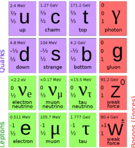
The Standard Model classifies the fundamental particles of matter in groups of one-half spin fermions and integer spin bosons. With a total of 12 fermions categorised further into two groups of six particles, called leptons and quarks, the ordinary matter is described. These two groups are separated based on the electric charges and the forces through which they interact with each other. Fig. 1.1
represents these fundamental particles along with the bosons that mediate the interactions between them in the Standard Model framework. One can divide this table into three generations of fermions. The first column corresponds to the particles of the first generation. The second generation is shown in the column two and the third in column three. Protons and neutrons are made of particles from the first generation. The other generations of elementary particles compose other kind of particles with a relatively short-life span. As to why there are three generations of particles, no one knows the answer. Each of this 12 fermions have an opposite partner with equal mass which are the respective anti-particles. These anti-particles defer from their partners in all the quantum numbers, with exception for the spin, being the opposite of its partner.
Figure 1.1: List of fermions and the respective bosons which mediate the interactions between them.
The gauge bosons are shown in the fourth column and are the mediators of the three forces. The photon is the mediator of the electromagnetic force and mediates the interaction of particles with electric charge. The Z and the W bosons are the mediators of the weak force through which one can explain the decay of all the short-lived particles. The gluon is the particle that mediates the strong interactions between particles that carry colour charge. The interaction range varies from each of the three forces. The electromagnetic force has infinitum range, while the other two forces have their interaction range smaller than 10−15 m. The gluon is the only boson of the mediators which can interact, not only with quarks, but specially with other gluons. Hadrons are composed of partons (quarks and gluons). Bound states of three quarks form baryons, such as the proton or the neutron, while combinations of a quark and an anti-quark yield meson particles, such as pions. While leptons carry integral electric charges, quarks carry fractional charges.
Colour confinement prevents the detection of single isolated quarks and gluons in nature. When a quark is ejected from a hadron in a high energy collision, the energy of the gluon connecting the two particles increases to the point where it breaks and spontaneously creates a quark-antiquark pair. The new emitted hadron then may radiate gluons, creating a collimated spray of particles commonly referred to as a jet.
In hadron-hadron collision two interaction types can be distinguished, soft and hard interactions. A soft interaction happens when the scatter between the two
hadrons results on two outgoing particles with low transverse momentum1 and with a small deviation angle. On the other hand, a hard scattering event is a process which probes very short distances within the hadrons. In this process partons are scattered at wide angles after passing very close to each other, and two or more high transverse momentum outgoing partons are produced. These partons hadronize and are observed as jets in the detector. Fig. 1.2 represents a typical hard scattering interaction between two incoming partons. Other soft interactions also play a role in the collision. The incoming partons may start of a sequence of branching (a process similar to Bremsstrahlung), which produces an initial state radiation shower. This branching also can happen after the hard scat-tering thus producing final state radiation. The partons not involved in the hard interaction scatter with small angles respectively with small transverse momen-tum. These partons are associated to the underlying event. Multiple interactions can contribute to the underlying event, usually this is identified as pile-up which is a feature that happens when two or more collisions happen in the same event. Minimum bias events are characterized by having only soft scattering collisions, thus producing only low transverse momentum particles.
The clear understanding of the soft processes is important for the correct mea-surement of the high transverse momentum hard scattering partons. The presence of the soft interactions and final hadronization of all colour connected constituents of the events, prevent us from observing a direct and exact measurement of the transverse momentum of the outgoing partons from the hard scatter. What is accessible for measurement is a collimated spray of particles, the jet, along with the collision background.
1.2
Heavy Ion collisions
The goal of colliding heavy nuclei at the LHC is to recreate the state of matter that is thought to have happened a few microseconds after the Big Bang. At this time, the temperature of the Universe was so large that quarks and gluons moved freely in a state of matter called Quark Gluon Plasma(QGP). As the Universe cooled down, the quarks and gluons became bound to the nucleons by the strong force. The heavy ion collisions aim to study that state of matter which is characterized by 1Transverse momentum is the particle’s momentum relative to the transverse plane of the
Figure 1.2: Jet production in a hard scattering event[6].
high temperatures and densities. However, atomic nuclei are spatially extended objects in comparison to the Hydrogen nucleus. An important feature of the nucleus-nucleus collisions is the impact parameter, b, the distance between the geometric centre of the two nuclei measured in the transverse plane of the collisions direction.
1.3
Proton-nucleus collisions
Proton-nucleus (p+A) collisions have a crucial importance in Heavy Ion Collisions. They serve as benchmark to interpret some of the main features of A+A collisions. The p+A physics are also of interest by their own allowing the study of nuclear Parton Distribution Functions (nPDF). Namely, gluon saturation and shadowing, among others.
1.3.1
p+A as benchmark for Heavy Ion collisions
Proton-nucleus collisions (p+A) are a crucial component of the heavy-ion program. They serve as benchmark to nucleus-nucleus collisions (A+A) to disentangle initial state effects in the nucleus, which are observed in p+A and also happen in A+A, from the hot and dense state of matter produced in A+A collisions. p+p collisions are used to study the interaction between partons in vacuum. p+A collisions are used to study the parton interaction within a nuclear environment. A+A collisions are used to study the interaction between partons in the Quark Gluon Plasma state of matter. The usual procedure is to study ratios of observables between the nucleus-nucleus or proton-nucleus and p+p cross sections scaled by the number of binary nucleon-nucleon collisions, Ncoll. The purpose is to distinguish cold nuclear
matter effects that happen in both p+A and peripheral A+A collisions, from the ones produced in central A+A collisions, in which the QGP is expected to occur. These ratios constitute the so-called nuclear modification factor, RAA, a
measurement of how the medium can modify the scaling between p+p collisions and p+A or A+A collisions. RXX is defined as:
RXX(pT, η) = 1 hNXX coll i d2NXX/dp Tdη d2Npp/dp Tdη (1.1)
where XX is the collision type one is studying, and can be A+A, p+A or d+A collisions. d+Au collisions at the Relativistic Heavy Ion Collider (RHIC) were used as benchmark in Au+Au collisions and have shown evidences of the jet quenching hypothesis, caused by the QGP, as a genuine final state effect. In central nucleus-nucleus collisions a deficit of high transverse momentum hadrons is observed while this effect is absent in the transverse momentum spectra of the inclusive hadron production in d+Au collisions [7]. To characterize the effects of cold nuclear matter, one has to have a precise knowledge of the PDF both the proton and the heavy nucleus. While in the proton case the PDFs are constrained by a large number of data from HERA and the Tevatron, in the nuclear case this is not true. Much less extensive experimental data on nuclear deep inelastic scattering (DIS) are available in the perturbative region (Q2 ≥ 1 GeV2) and only
for Bjorken-x (x) > 0.01 [8]. The LHC assesses completely unexplored regions of the phase space of the nuclear PDF (x < 0.01). And so, for a contribution to the understanding of the hot partonic matter produced in Pb+Pb collisions,
one should also study p+Pb collisions in order to remove the uncertainties of the nuclear PDF.
With the LHC, the TeV scale is achieved for the first time. This unexplored kinematical regime translates into a untapped reach of Bjorken-x and virtuality Q2 in several orders of magnitude, which allows the study of the nuclear PDF at
lower x values.
1.3.2
Centrality
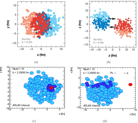
The centrality of a collision can be perceived as a measure of the topology of a collision. In contrast with p+p collisions, when colliding two heavier nuclei one can have distinct events, depending on the impact parameter b of the two nuclei. The objective of estimating the centrality variable is to identify those events and to each one attribute the correspondent centrality class. A simulation model of a collision between two gold nuclei viewed in its transverse and longitudinal plane is depicted in Fig. 1.3(a) and Fig. 1.3(b). For large b collisions it is expected a low number of binary collisions between the nucleons which leads to a low number of particles in the event, while for small b collisions it is expected high number of collisions and the resulting larger number of particles. The number of particles in an event is associated with underlying event at the detector level. Figs. 1.3(d)
and 1.3(c) show a simulation of a p+Pb collision.
The characterization of the centrality variable in A+A or p+A collisions is performed considering the Glauber Monte Carlo model [1] which is inspired in the Glauber model[9]. The Glauber Monte Carlo model considers the nucleus as group of uncorrelated nucleons taking into account the density distributions of the nuclei. The collision model considers a random impact parameter b and assumes that the nuclei follow a straight line until the collision. The interaction probabil-ities between the nucleons of each nuclei is performed using the relative distance between them. This collision model considers as main inputs the nuclear charge densities following a Fermi distribution and the energy dependence of the inelastic nucleon-nucleon cross section. The nucleon-nucleon cross-section is assumed to be equal to the proton-proton inelastic cross-section.
(a) (b)
(c) (d)
Figure 1.3: A Glauber Monte Carlo model of a Au+Au collision event is shown in Fig. 1.3(a) in a transverse view and in Fig. 1.3(b) in a longitudinal view [1]. Fig.1.3(c) and 1.3(d)show a model of a p+Pb collision event[2].
A“participant” is a nucleon which interacts at least once in a given collision. The number of participants (Npart) is the total number of nucleons which
inter-act in a collision, while the number of binary collisions (Ncoll) is the number of
interactions that all nucleons in a given nucleus experience. In nucleus-nucleus (A+A) collisions there are proportional relations between both Npart and Ncoll
and the impact parameter, and between the parameters Npart and Ncoll as well
as the number of produced particles (multiplicity). In p+A collisions the relation between Npart and Ncoll and the impact parameter is not so straightforward.
With the Glauber Monte Carlo model one can get Npartand Ncoll distributions
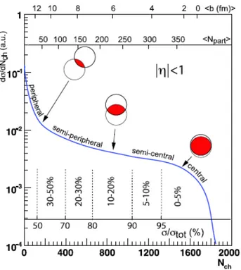
by simulating many nucleus-nucleus collisions with different impact parameters. Once these distributions are obtained, they are fitted to the experimental data. A measured distribution (e.g., dNevt/dNch or P ETEvt ) is mapped to a distribution
’centrality classes’ in both measured and simulated distributions. Fig.1.4shows an illustrative representation of the correlation between the distributions of Npart and
the number of charged particles (Nch). The mean values from the same centrality
class in the two distributions allows one to separate the different centrality classes. Usually the distributions are divided in percentiles, such that each percentile is a fraction of the total inelastic cross-section. The ’centrality class’ of an event is classified between 0 to 100%.
Figure 1.4: Correlation between the distributions of the number of partic-ipants in a binary collision (Npart) and the number of charged particles in a
Minimum Bias sample (Nch) are shown. Percentiles of the distribution are also
applied in this distribution with no criteria[3].
1.3.3
Jet production
Jets are most often produced in pairs, well-balanced in azimuth and transverse energy (ET), at leading order and in absence of energy loss. They are the
domi-nant contributor to the total jet production cross-section of hard-scattering events. However, if the hard scatter occurs in the Quark Gluon Plasma (QGP) medium as the one produced in ultra-relativistic heavy ion collisions, the partons lose energy
while traversing the medium, by interactions or induced gluon radiation. This phenomenon is commonly referred to as jet quenching.
One of the many ways to study the jet quenching is the study of dijet asym-metry distributions between the most leading ET jets in an event, in separate
cen-trality classes. This result shows that while in peripheral collisions the asymmetry distributions are well balanced in ET, in central collisions the same distributions
show no balance between the transverse energy of those jets. More information regarding this topic can be seen at [10].
RCP measurements is also another study to analyse the jet quenching
hypoth-esis. It is defined as the ratio of the differential yields in some centrality class collision to the most peripheral ones, both normalized to the corresponding num-bers of binary collisions. The RCP between central and peripheral collisions is
defined as: RCP(pT, y) = hNcollP eripherali hNCentral coll i d2NCentral(p T, y)/dpTdy d2NP eripheral(p T, y)/dpTdy (1.2)
The jet yield is found to be suppressed by approximately a factor of two in the 0-10% centrality class relative to peripheral collisions. RCP varies smoothly with
centrality as characterized by the number of participating nucleons. The observed suppression is only weakly dependent on transverse momentum[11].
1.3.3.1 Jets in p+A collisions
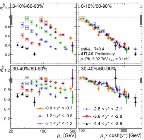
The jet production in p+Pb collisions is found to be also dependent on centrality and rapidity[12]. In this reference results of central-to-peripheral ratios, RCP, as
a function of the jet transverse momenta, for different slices of jet rapidity, are presented. Results of this measurement indicate a strong, centrality-dependent reduction on the yield of jets in central collisions relative to that in peripheral collisions. This reduction becomes more pronounced with jet pT and at more
forward (downstream proton) rapidities, as presented in Fig.1.5
The goal of this dissertation is to study the ATLAS jet trigger in this environ-ment, that is dependent on variables such as the centrality class of the collision, the rapidity and transverse energy of the jet, among others.
Figure 1.5: RCP for R=0.4 jets in p+Pb collisions at
√
sN N = 5.02 TeV.
Each panel shows the RCP in jets in multiple rapidity bins at a fixed centrality
interval. The top row show the RCP for 0-10%/60-90% and the bottom row
show the RCP for 30-40%/60-90%. In the left column, the RCP is plotted
against jet pT. In the right column, the RCP is plotted against the quantity
pT × cosh(y∗) where y∗, the rapidity measured in the center of mass frame, is
the midpoint of the rapidity bin. Error bars on data points represent statistical uncertainties, boxes represent systematic uncertainties, and the shaded box on the RCP=1 dotted line indicates the systematic uncertainty on Ncoll for that
Experimental Setup
The European Organization for Nuclear Research (CERN) is a scientific research facility located near Geneva, Switzerland. At CERN exists an accelerator complex in which several experiments were built to study the basic constituents of matter.
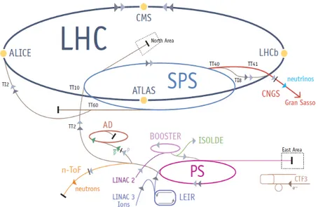
Figure 2.1: Schematics of the accelerator complex at CERN. Several acceler-ators are used to achieve higher beam energies. The proton beam acceleration chain can be seen by following the light blue arrows from Linac2. While the
208Pb beam chain is depict in the dark blue arrows starting in Linac3.
The accelerator complex consists on a chain of accelerator machines, linear and circular accelerators, where the next machine brings the particle beam to a higher energy. The last element of this chain is the Large Hadron Collider (LHC), with a
circumference of 26.7 km. ATLAS, CMS, LHCb and ALICE experiments are found in the LHC ring. In these experiments the beams are forced to collide with each other. Other experiments are carried in relatively smaller accelerator machines using beams of lower energies, such as ISOLDE and COMPASS experiments. A schematics of the accelerator complex is shown in Fig. 2.1.
2.1
The Large Hadron Collider
The basic structure of matter can be described by the Standard Model of Particle Physics[14]. However this is an incomplete model. The LHC was built and de-signed to provide with some answers that this model doesn’t consider, such as the existence of dark matter and dark energy in the universe, test the super-symmetry model, hot quark matter, among others. These subjects are studied by making proton-proton or lead-lead collisions in the LHC.
The LHC machine structure [15] consists of two parallel beam pipes where protons and/or 208Pb nuclei circulate in opposite directions. The beam pipes
cross at four specific points, called interaction points (IPs). In each point the beam constituents are made to collide and the experiments which are centered around the IPs are used to record the results of the collisions. In order to diminish random collisions with air molecules, the beam pipes are kept at ultra-high vacuum conditions reaching an average of 10−13 atm.
The counter-rotating beams are contained within a single magnetic structure. The particles orbits are controlled by 1232 magnetic dipoles and the focus of the beam constituents in the transverse plane is maintained by 392 quadrupole mag-nets using an alternating field. These are superconducting magmag-nets that operate at 1.9 K. The LHC holds 8 radiofrequency (RF) cavities per beam. These are responsible for the acceleration of the beam to the largest energy and guarantee high luminosity at the interaction points.
Before reaching the LHC, protons follow a certain accelerator chain that is depicted in Fig.2.1. Protons are obtained by stripping the electrons from hydrogen atoms and can be accelerated to an energy of 50 MeV in the linear accelerator Linac2. Later, protons are injected to the Proton Synchrotron Booster (Booster) where they are accelerated up to 1.4 GeV. Energies of 25 GeV are then reached
at the Proton Synchrotron (PS). At the Super Proton Synchrotron (SPS) protons are accelerated to 450 GeV. Finally, in the LHC energies of 4 TeV can be reached. Regarding the 208Pb ions, these are produced from an heated sample that is
primarily ionized by an electron current. This ionization can reach the state of Pb29+. An additional ionization is reached by impinging the Pb ions on a carbon
foil. The stripped ions are fed to the Low Energy Ion Ring (LEIR). The ions are injected to the PS with an energy of 72 MeV/u where the beam is accelerated to 5.9 GeV/u. Only after passing a second foil, in order to achieve a complete stripping, the beam is injected to the SPS. The beam is sent to the LHC with an energy of 177 GeV/u where it is accelerated to 1.38 TeV/u. This scheme of injection is also shown in Fig. 2.1.
A beam might circulate about 10 hours in the LHC. The hadrons circulate in the ring in bunches due to the RF acceleration. In this type of accelerators the ions can be accelerated only when they pass a cavity and the RF field has a certain orientation. In the LHC, the proton beams are made of 2808 bunches, each bunch contain 1011 protons.
The size of the bunches varies within the ring, being reduced around the in-teraction point in order to increase the probability of collision at each of the four interaction points.
2.2
ATLAS
2.3
Detector Overview
ATLAS [16] is a multi-purpose particle detector that is located at the Interaction Point 1 (IP 1) of the LHC. It is 25 m high, 44 m long and weighs approximately 7000 tonnes. The detector was designed to identify and measure all the products of the collisions of the beam particles. Its main purpose is to verify the Standard Model (SM) and probe for physics beyond the SM. ATLAS is able to study p+p, Pb+Pb and p+Pb collisions.
The ATLAS detector is organized in layers surrounding the interaction point. From the inside to the outside, it consists of the following subdetectors: the Inner
Detector, the Magnet System, the Electromagnetic and Hadronic calorimeters and the Muon Spectrometer, which in their turn are composed of more sub-detectors. A schematic view of the complete layout of the ATLAS detector can be found in Fig.2.2. The Electromagnetic, Hadronic calorimeters and the Muon Spectrometer are divided into barrel and end-cap detectors. In the barrel the detectors are arranged in concentric cylinders, around the beam axis, while the end-cap detectors are imprinted in disks perpendicular to beam axis located at the ends of the barrel. The variables used to map and limit the detector are the (η,φ) coordinate system and are defined in App.A along with some other used variables.
Figure 2.2: Overview of the ATLAS detector where the main sub-detector systems are identified.[16]
Another important parts of the ATLAS detector are the software and hardware components to digest the millions of events per second. Nowadays such a high rate of events that is delivered by the LHC is impossible to record completely. The trigger and the data acquisition systems aim to select potential interesting events to save, according to the physics one is interested in.
In the following sections the different components of the ATLAS detector will be briefly introduced with exception for the calorimeters, which due to the rele-vance for this dissertation are extensively exposed.
2.4
The Inner Detector
The Inner Detector (ID) is the first detector system that surrounds the high-radiation area near the IP. The ID is composed of a set of subdetectors: the Pixel Tracker, the Semiconductor Tracker (SCT) and the Transition Radiation Tracker (TRT). A schematic view of the ID is shown in Fig2.3.
Figure 2.3: Overview of the Inner Detector and its detection subsystems: the Pixel Tracker, the Semiconductor Tracker (SCT) and the Transition Radiation
Tracker (TRT)[16]
The purpose of the ID is to accurately identify and reconstruct the trajec-tories of charged particles, combining high-resolution detectors near the IP with tracking elements at a larger radii. The detector subsystems are all immersed in a 2 T nominal magnetic field provided by the Central Solenoid Magnet. This al-lows to measure with excellent resolution the momentum of the charged particles. Precision vertex reconstructions are also achieved with the ID.
Due to its working environment, i.e., high radiation area, the detector takes advantage of fast and radiation-hard electronics and sensors.
The next paragraphs summarize each of the sub-detectors that compose the ID.
The Pixel Tracker is the first layer of the ATLAS detector. It is a radiation hard semiconductor detector that measures all tracks within a |η| < 2.5 region. It uses 80 million silicon pixel sensors to provide high granularity in the barrel region, each pixel sensor with a 50 × 400 µm2 area. The vertexing layer is the
closest to the interaction point, and provides precision measurements over the full acceptance. The Pixel Tracker is crucial to identify and reconstruct the primary and secondary vertices, due to its proximity to the interaction point and highly segmentation, allowing a flavor-tag analysis (e.g. identifying B-Hadrons).
The Semiconductor Tracker is a silicon micro-strip detector that is placed at a larger radii than the Pixel Tracker enclosing it. It also contributes to the measurements of momentum, impact parameter and vertex position.
The Transition Radiation Tracker is the outermost subdetection system of the ID. It is composed of gaseous straw tube detectors. The barrel TRT straws are parallel to the beam direction, while all end-cap tracking elements are located in planes perpendicular to the beam direction. Each straw is filled with a gas mixture with 70 % of xenon. The straws are within a matrix of polypropylene fibres. When a charged particle passes through the polypropylene photons are produced. These ionize the gas in the straw tubes and the collected signal is then read out. This detector not only provides high resolution momentum measurements but also identifies electrons based on the photon signature when traversing the drift tube.
2.5
Calorimetry
Calorimeters are used to measure accurately the position, time1 and energy of particles by their absorption. Calorimeters are used in high energy physics to measure the energy of all hadronic and electromagnetic interacting particles. They can account for missing transverse energy and also provide fast and efficient trigger output. Some of the most important features include energy resolution, position resolution, signal speed, Gaussian response signals and a good known relationship between the energy and signal. The energy resolution improves with energy which 1A time measurement relative to the LHC clock can be measured for some ATLAS detector
is proportional to 1/√E in a calorimeter, in contrast with a magnetic spectrometer which has the momentum resolution proportional to p.
Calorimeters are designed according to the interaction processes and the ex-pected particle energy. Different interaction processes may occur for electromag-netic and hadronic particles at a given energy. In the case of electrons, positrons and photons, the energy loss is dominated by electromagnetic interactions. In the case of strong-interacting particles the energy loss processes are substantially more complex than the electromagnetic case. The reason lies in the larger variety of strong processes that may occur at the particle level and with the interacting nucleus and also electromagnetic interactions. Moreover, not all the energy loss caused by strong processes can be measured as it will be discussed.
When a high energy particle interact with the calorimeter material it will create additional particles through several processes, not necessarily in the same direction as the primary particle. In their turn these secondary particles create further particles. This process repeats itself until the last created particle has insufficient energy to create more particles. The entire process of production of particles constitutes a particle cascade or shower. This shower of particles develops until all particles are completely stopped. At this stage almost all the energy of the primary particle is deposited.
2.5.1
Electromagnetic Showers
An electromagnetic particle shower happens by several different processes. The dominant energy loss for photon in electromagnetic processes are the photoelectric effect (occurs with more probability at low energies), the Compton scattering (is more likely to occur in the keV to MeV energy scale) and the pair production (this process happens at energies larger than 1 MeV). The principal source of energy loss in electrons and positrons at 100 MeV is bremsstrahlung when the electrons interact with the electric fields of the atomic nuclei of the calorimeters. This process generates many soft photons that are absorbed by Compton scattering or photoelectric effect, and a few energetic photons that will produce an electron-positron pairs. These soft particles in a shower carry most of the electromagnetic energy of the primary particle.
The electromagnetic cascade is characterized by the radiation length (X0), the
longitudinal spread and transverse spread. The radiation length can be perceived as the distance travelled in which an electron looses on average 1 − e−1 of its energy. In the case of a high energy photon, X0 is the mean free path in which a
electron-positron pair is produced with a probability of 7/9. The radiation length is proportional to the mass number and the atomic mass, X0 ∝ A × Z−2, thus
calorimeters are designed with high Z materials such as lead, in order to minimize the shower length and absorb it completely. The radial spread is determined by the Moli`ere radius (RM), which is a function of X0 and EC. Roughly 90% of the
energy is contained inside a cone of radius RM around the shower’s axis.
2.5.2
Hadronic Showers
Hadronic showers are more complex than the electromagnetic showers. Not only we have to account for the energy losses of the incoming hadron but also account for the energy loss with the nuclei whom the hadron interacted. Regarding the incoming particle, some high energy neutral hadrons may decay in to photons and charged hadrons suffer energy loss through ionization of the medium. This means that an hadronic shower usually contains electromagnetic component. On the other hand the interacting nuclei also accounts for energy loss by spallation reactions and the nuclear binding energy associated with that reactions. The detection efficiency of the hadronic calorimeter is, in general, worse than in the electromagnetic. Undetected energy losses can happen due to neutral particles such as neutrinos and slow neutrons; backscattered charged particles and muons that escape the hadronic calorimeter completely.
The hadronic shower contain an electromagnetic component which has a differ-ent shower developmdiffer-ent and overall calorimeter response. The non-compensation between the two components has to be accounted for. The non-electromagnetic component of the hadronic shower can either be not detected totally or often too slow to be within the detector time window. This will not only destroy the cor-relation between the primary particle energy and the detector response but also decrease the energy resolution, making it gaussian. Experimentally this non-compensation is determined by signal tests of e/π ratios at different energies and applying calibration parameters to the measured energy.
In hadronic showers, the nuclear absorption length λ0 is the equivalent
param-eter of the radiation length X0 in electromagnetic showers. λ0 is the mean free
path before an inelastic interaction occurs and is proportional to the inverse of the density of the material and the nuclear inelastic cross-section. Usually the absorp-tion length is larger than the radiaabsorp-tion length which requires hadronic calorimeters to be larger.
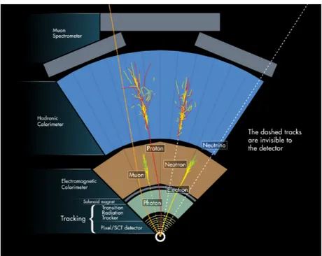
Fig. 2.4 shows different types of particles and their typical behaviors in inter-acting with the ATLAS detector, and more specifically their interaction with the calorimeters material as described in this section.
Figure 2.4: Particle detection in the hadronic and electromagnetic calorime-ters of ATLAS. Showers produced by a photon and electron in the electromag-netic calorimeter and the hadronic showers induced by a proton and a neutron
in hadronic calorimeter are shown [16].
2.5.3
ATLAS Calorimeters
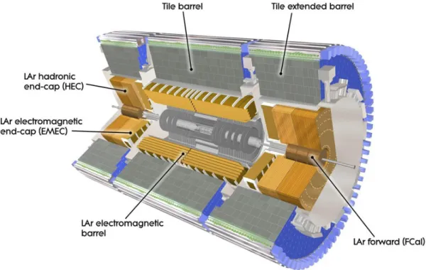
The ATLAS detector is composed of two main sampling calorimeter systems: the Electromagnetic calorimeter and the Hadronic calorimeter. Both calorimeters have backward-forward symmetry and are grouped in two distinct parts: the barrel and two end-caps. The barrel part is concentric around the axis beam, and end-caps which are placed at both ends of the barrel and are perpendicular to the beam pipe. Fig 2.5 represents a schematics of the ATLAS calorimeters [16].
ATLAS electromagnetic and hadronic calorimeters were built with alternat-ing stacks of absorption material layers followed by detection devices, which are commonly known as sampling calorimeters. Using different absorption materials, different particles can be measured such as photons, electrons and hadrons. Other particles, such as neutrinos and muons, deposit none or little energy loss in the calorimeters. In the case of neutrinos, their energy can be inferred from the missing transverse energy as these calorimeters are hermetic detectors. Sampling calorime-ters, when compared to homogeneous calorimecalorime-ters, which are characterized by a medium which is simultaneously active and passive, allow a better segmentation and cope better with radiation damage to the detector. On the other hand they have worse energy resolution and record only the part of the energy deposited in the active medium.
The segmentation of the calorimeter allows the determination of the 4-momentum vector of the particles. The signals collected in different cells allow a definition of the shower axis and thus the direction of the particle that traversed that medium. The material from which the calorimeter is made determines the different types of signals used.
The calorimeters were designed with two distinct technologies: liquid argon technology and tile scintillators. In the liquid argon technology a particle is de-tected by ionizing the cryogenic liquefied noble gas in the active medium and the absorber is composed of lead laminated with steel support plates. The tile scin-tillator technology uses steel plates as passive material and scintillating plastic tiles as its active medium. As the particle passes through the scintillating tile, light is produced and a wavelength shift fiber will re-emit the light with a longer wavelength (lower energy) and delivered to the photomultiplier module.
2.5.3.1 Electromagnetic Calorimeter
The electromagnetic calorimeter (EM) in ATLAS is composed of the electromag-netic barrel (EMB) component and two electromagelectromag-netic end-caps (EMEC) com-ponents. All of these components employ the liquid argon technology. The EMB has a sampling calorimeter in front of it, called the Pre-Sampler, which is used to improve the measurement of the lost energy by photons and electrons.
Figure 2.5: Overview of the ATLAS Calorimeters: Electromagnetic and Hadronic. The technologies used were Liquid Argon (LAr) and tile, these are
also indicated for each calorimeter component[16].
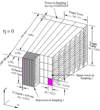
The Electromagnetic calorimeter also provides high granularity and good her-micity due to its ”accordion geometry” in the passive material, as can be seen in Fig.2.6. This geometry is symmetric in φ and more importantly doesn’t allow for any azimuthal cracks in the calorimeter.
The Electromagnetic Barrel surrounds the Central Solenoid Magnet and has a coverage of |η| < 1.475. It is composed of three concentric layers with different granularities in η and φ, having area cells of 0.025 × 0.0245. In the central region of |η| < 2.5 the EM calorimeter has three longitudinal sampling layers with different segmentations.
The EMEC are placed at each side of the barrel and covers 1.375 < |η| < 3.2. Regarding the granularity, the EMEC are also highly segmented in η and φ, having area cells of 0.025 × 0.0245 in the η × φ phase space.
The radiation length associated to the EM calorimeter has a minimum of 24 X0 in the EMB and 26 X0 in the EMEC. [17].
Figure 2.6: Perspective view of the EM calorimeter segmentation. The ac-cordion geometry allows the calorimeter to not have azimuthal gaps, is φ-symmetric, and adding an highly segmentation to identify precisely the position of the particles that traverse the material, results in a great accuracy of energy
measurements[16].
2.5.3.2 Hadronic Calorimeter
The Hadronic calorimeter is the the next detector system that surrounds the EM. It is divided in two subsystems; two hadronic end-caps (HEC) and the Tile Calorime-ter (TILECAL) which in turn is divided in Hadronic Barrel (HB) and hadronic extended barrel (HEB). Between the hadronic barrel and hadronic extended barrel lies a crack of 68 cm in which are service pipes, Inner Detector supporting cables as well for the solenoid magnet and for the electromagnetic calorimeter.
The TILECAL uses polystyrene scintillating tiles technology and steel as active and passive mediums respectively. The tile planes are oriented perpendicularly to the beam axis and are radially staggered in depth as it can be seen in Fig 2.7. This geometry of modules provides an uniform signal response of the calorimeter and hermetic coverage.
Figure 2.7: A tile calorimeter module composed of the steel absorbers, the scintillating tiles, the wavelength shift fibers and the photomultipliers[16].
TILECAL has three sampling layers in the longitudinal direction. The group-ing of the tiles and photomultiplier tubes allows a segmentation in η and φ. The resultant granularity for these modules is 0.1 × 0.1 in the η × φ plane. Also, the TILECAL has an interaction length minimum of λI = 7.4 in its η-central region.
2.5.3.3 Hadronic end-caps
The hadronic end-caps are symmetric in ± z and are located after the electro-magnetic end-caps. The difference between these modules, the electroelectro-magnetic end cap and the hadronic end cap, lies in their sampling materials. The hadronic end cap is composed of liquid argon technology as the active medium and as a passive medium copper to increase the interaction length in comparison to the EM Liquid Argon system. The HEC share the cryostat plates with the EMEC and the forward calorimeter. Being composed of two independent wheels and these extend the η coverage 1.5 < |η| < 3.2. However the segmentation is different for
different η ranges: for |η| < 2.5 is η × φ = 0.1 × 0.1, while for 2.5 < |η| < 3.2 it is η × φ = 0.2 × 0.2.
2.5.3.4 Forward Calorimeter
The main purpose of the Forward Calorimeters (FCal) is to extend the acceptance of the detector in η and probe physics at forward pseudorapidity. The FCal range in η is 3.1 < |η| < 4.9. This increase in |η| allows for more more accurate missing transverse energy measurements. The FCal is also of great importance in Heavy Ion collisions, as it is the detector in which it is defined the centrality of the collision. The FCal are located between the beam pipe and the hadronic end caps, being z-symmetric (the axis in the direction of the collision axis). Each of them is segmented along the z axis in 3 sections; the closest to the interaction point is regarded has a sampling electromagnetic calorimeter, being composed of stacks of liquid argon and copper as the active medium and absorber respectively. In respect to its hadronic part, it is segmented longitudinally in 2 sections, the active mediums and passive mediums are liquid argon and tungsten made. The granularity in the η × φ plane is 0.2 × 0.2. It has a high radiation level formed of low transverse energy particles with high energy. The detector was designed with a fast response to minimize the effect of pileup from either a previous bunch crossing or multiple hard scattering event.
2.5.4
Minimum Bias Trigger Scintillators
The Minimum Bias Trigger Scintillator (MBTS) is a calorimeter which is made of only active medium. Composed of two z-symmetric components, they are installed at the ends of the Inner Detector at ± 3.6 m, and cover a range from 2.09 < |η| < 3.84. The main purpose of this detector is to select interesting events by requiring a minimum number of hits. It can be also used in offline analysis to reject out of time signals, considering the timing of the signal measurement relative to the LHC clock time.
2.5.5
Zero Degree Calorimeters
The Zero Degree Calorimeters (ZDC) are sampling calorimeters installed at ± 140 m, just beyond the beam pipe splits. They cover a range of |η| > 8.3. These detectors are mainly used in Heavy Ion Collision experiments. They can measure spectator neutrons in lead-lead collisions that are not deviated in the magnetic fields of the beams, as charged particles and nuclei. It can also be used to trigger interesting events by requiring a hit, and thus reject photonuclear collisions, beam gas and beam halo effects.
2.6
Muon Spectrometer
The Muon Spectrometer (MS) is the last detector that is surrounding the beam pipe. It is designed to detect muons that are created in the hard scatter. It can be used to identify the position, momentum and the signal of all the charged particles that are not absorbed by the hadronic calorimeters. A scheme of the Muon Spectrometer can be found in Fig. 2.8.
Interspaced with the Muon spectrometer are found three large Semiconductor Toroid Magnets (SCT Magnet), one at the barrel region and two at the respective end caps. In contrast with the Central Solenoid Magnet which has a constant magnetic field, the SCT Magnets haven’t and the barrel toroid magnet (|η| < 1) can vary from 0.2 T to 2.5 T in its bore, while the end cap toroid magnets (1.4 < |η| < 2.7) the maximum value is 3.5 T. In the transition region between the barrel and end-caps (1 < |η| < 1.4), the magnetic field is generated by the two magnetic systems and has an average field of 1 T.
The Muon spectrometer has four types of detectors, two of them located in the barrel region: the Resistive Plate Chambers (RPC) and the Muon Drift Tubes (MDT) and two in each the end caps: the Thin Gap Chambers (TGC) and a system composed of the MDT and Cathode Strip Chambers (CSC). The RPC and TGC systems were designed to provide the Muon Spectrometer a fast response but less accurate position measurements, ideal to trigger muon objects. On the other hand, the MDT and the CSC have accurate tracking of the position, momentum and charge measurements.
Jet Trigger System
An overview of the entire trigger and data acquisition system is presented in the first section. The following sections present with some detail the jet trigger system, finishing with the presentation of the jet trigger menu for the 2013 p+Pb run.
3.1
Overview of the Trigger and Data
Acquisi-tion systems
The Trigger and Data Acquisition system (TDAQ) [16] plays an important role in the ATLAS detector as it manages the processing of data streaming. With current technology it is impossible to record all events of a designed collision rate of 40 MHz, therefore the TDAQ system is required. This system was designed to reduce the input data rate to approximately 200 Hz which corresponds to approximately 300M B/s devoted to offline storage and processing of the data. With the develop-ment of new software and hardware components, the input data rate was increased to 400 Hz during the p+Pb data acquisition. In these few hundred Hertz the aim is to select interesting and rare events for offline analysis. This corresponds to a factor of 107 reduction of the data rate and with a latency of only a few seconds.
The ATLAS trigger system is comprised of three levels, each one adding more complexity to the previous. The Level 1 (L1) is the first level and is a hardware-based system that uses information from both electromagnetic and hadronic calorime-ters and the muon spectrometer sub-detectors. The second and third levels of the ATLAS trigger system are known as Level 2 (L2) and Event Filter (EF). Both
subsystems are software based, and use not only information from the calorime-ters and muon systems but also from the Inner Detector. Together, L2 and EF are known as the High Level Trigger (HLT).
The trigger system is responsible for the event selection that fulfils at least one of the thousands possible conditions (triggers) at each bunch crossing. There are triggers designed to identify electrons, muons, photons, jets, or select specific jets (e.g. jets with b-flavour tagging or specific B-physics decay modes). There are also triggers specialized in global event properties such as summed transverse energy (P ET) and missing transverse energy (ETmiss), the latter commonly associated
with neutrinos.
A schematic diagram of the ATLAS trigger system is presented in Fig. 3.1
Figure 3.1: Schematic diagram of the ATLAS trigger system. The three trigger levels (L1, L2 and EF) aim to select and record a broad variety of rare
physics events from a designed 40 MHz bunch crossing rate.[18]
The L1 Trigger is built with fast custom trigger electronics in order to get a latency of less than 2.5 µs, reducing the rate to a maximum of 75 kHz. From the information of the calorimeters and muon tracks the L1 trigger identifies and selects Regions of Interest (ROI) which are used in the next trigger levels.
The HLT is a commodity computing system connected by fast dedicated net-works. After the L1 trigger selection, the data from each detector is transferred to a detector-dedicated Readout Buffer (ROB), which stores the event depending on the L2 decision. A set of ROBs are gathered in the Readout systems (ROS) and are connected to the HLT networks. The L2 trigger which is based on fast custom algorithms, process the data only within the ROIs from L1. The ROS send the data to L2 upon request, which is associated to detector elements inside each ROI. This results in a considerable reduction of the data processed and transferred to L2. The L2 has a latency of 40 ms and its designed rate is 3 kHz.
All events that pass the selection criteria at L2 are passed to the Event Builder which reads out the data from the entire detector assembling all the different parts of data from the ROBs. The full event data is processed by the last stage of the trigger system, the Event Filter. It consists of a farm of commodity processors that runs faster or modified versions of offline algorithms. The EF reduces the event rate to at most 400 Hz with an average processing time of a 4 seconds/event.
After processing the data at the EF, the events selected by the trigger system are written to data streams with dedicated trigger types. Usually data streams are separated in two types, physics data streams and calibration data streams.
Four primary physics streams were configured in the 2013 p+Pb run:
• MinBias: the Minimum Bias stream, which recorded minimum bias and high-multiplicity triggered events from various subsystems including the MBTS, ZDC, ID detectors, among others. The allocated bandwidth for this stream was 250 Hz.
• HardProbes: the HardProbes stream recorded events associated with elec-trons, photons, muons, jets and missing transverse energy and had an allo-cated bandwidth of 150 Hz.
• UPC : the ultra-peripheral collisions stream, which recorded events associ-ated with photo-nuclear processes, characterized by a low track multiplicity. This stream had a dedicated bandwidth of 10 Hz.
• MinBiasOverlay: the Minimum Bias overlay stream, had a 5 Hz bandwidth. This stream recorded a sample of minimum bias events that would be later embedded with PYTHIA Monte Carlo samples.
• Express Stream: about 10% of the events are written into the Express Stream. The prompt offline reconstruction of this data provides calibra-tion and Data Quality (DQ) informacalibra-tion prior to the reconstruccalibra-tion of the four physics streams that were defined before.
This dissertation focuses on the performance of jet triggers, recorded on the stream HardProbes, using the MinBias stream. The chosen stream allows for an unbiased sample of events which no other primary physics stream can offer. Moreover, the jet trigger chains aren’t defined in the MinBias stream but the trigger algorithms ran and the information of the event is recorded, thus one can emulate the trigger decision in order to study the jet triggers.
3.2
Trigger system configuration
The trigger system is configured by a trigger menu in which are defined trigger chains. These are composed of a sequence of conditions from the three trigger stages, that ultimately characterize the object triggered.
Each trigger chain has a specific rate, which is the number of times the object of interest is selected in a second. This rate has to be only a fraction of the maximum output rate of the EF and so prioritize the physics we are interested in recording. There are three ways of controlling the rates of a given trigger signature: by changing energy thresholds, applying different sets of selection cuts (e.g. isolated objects) or prescales.
Prescale factors can be applied to each level of the trigger. A prescale of 20 means that 1 in 20 events triggered will move to the next stage. Generally the rate depends on luminosity, therefore the prescale sets are automatically modified in each of the trigger levels to accommodate the change of luminosity, in order to maximize the bandwidth available and ensure a constant output rate.
To summarize, the trigger menu is developed according to the physics we are interested in recording. The prescales are automatically generated according to a set of rules that take into account the priority that each trigger chain has in the menu. The trigger chains can be categorized as: primary triggers, which select the events with the properties of the physics we are interested in and should not
be prescaled; supporting triggers, which serve as a support to the primary triggers (e.g. orthogonal triggers for efficiency measurements or prescaled triggers with of a lower ET threshold); Monitoring and Calibration triggers, used to collect data
used to evaluate the performance of the triggers and detectors.
3.3
Jet trigger overview
The ATLAS calorimeter trigger uses information from the hadronic and electro-magnetic calorimeters to identify and select localized objects (e.g. electron/pho-ton, tau and jet) and global transverse energy triggers. Due to the nature of this dissertation it will be only discussed the jet trigger system. Other trigger systems information can be found in Ref.[16, 17].
3.3.1
Level 1
The jet trigger is a subsystem of the ATLAS trigger, being the L1 trigger its first component. It reconstructs the jets using reduced granularity calorimeter information from both calorimeters, hadronic and electromagnetic. At L1 the energy in both calorimeters is calibrated only at the EM scale. The L1 decision is based on the information from analogue sums of calorimeter elements that define trigger towers. The trigger towers in each of the two ATLAS calorimeters are separate. The segmentation of the calorimeter is η dependent, therefore these trigger towers have different granularity in η. In the central region is approximately ∆η × ∆φ = 0.1 × 0.1 for |η| < 2.5. In more forward regions the granularity is broader. In the 2.5 < |η| < 3.2 the trigger tower size is ∆η × ∆φ ≡ 0.2 × 0.2, while in the FCal (3.2 < |ηk, < 4.9) there is no η segmentation and ∆φ ≡ 0.4. The jet and energy-sum processor uses 2 × 2 sums of trigger towers, called jet elements, to identify jet candidates. This means that there is a minimum resolution of 0.2 × 0.2 at η-central region, despite the smaller trigger tower size.
Jets Regions of Interest (ROI) are defined as 4 × 4, 6 × 6 or 8 × 8 trigger tower windows with its position defined in an 2 × 2 trigger tower area of maximum energy. The summed transverse energy also have to exceed a predefined threshold imposed in the trigger menu. This information will be then processed to make a global L1 trigger decision.
Figure 3.2: Sliding windows of the electron/photon and tau algorithms with its sums to be compared to programmable thresholds. The same procedure is used to identify L1 triggered jets with larger sliding window algorithms.[16]
Fig. 3.2 shows an example of a 4 × 4 sliding window, defined by 4 × 4 trigger towers. This sliding window is used to identify jet candidates and form global transverse energy sums.
3.3.2
Level 2
In the 2013 p+Pb run, the L1 output rates of the triggered jets were lower than the EF input rates. This allowed the L2 jet trigger to run in a pass-through mode, which means that although the L2 would run its algorithms, the event passed to the EF trigger stage despite the L2 decision. The menu for jet triggers is defined by a L1 jet trigger decision and/or a EF jet trigger decision chain, as we will see in due time. The information regarding the L2 jet trigger in this subsection will be only informative as it was not used in any time in this analysis.
In order to maintain a short period of the order of 40 ms processing per event, the L2 trigger jet system reconstructs and identifies candidate jets only within
the ROI defined in L1 and with a basic jet cone algorithm. The position and energy of each calorimeter cell within the ROI is read out and is used as input for the L2 cone-shaped jet reconstruction algorithm. This algorithm has a previously configured radius in the η × φ space. It takes into account all the calorimeter cells within the region of interest to identify and reconstruct candidate jets using iteration processes. It is the algorithm that will define the position and total energy of the L2 candidate jet. The total energy is calibrated at the hadronic scale.
3.3.3
Event Filter
The EF trigger is the last stage of the trigger where an event is either rejected or recorded. This stage happens after the Event Builder stage and has access to the entire detector granularity. Due to the rate that the EF has to process, it is possible to process events with almost the same level of detail as in offline, which is the event processing after the recording procedure.
The EF is a process with three stages. These are the data preparation, followed by a jet reconstruction procedure and the hypothesis testing defined in the trigger menu. These stages are shown in Fig. 3.3
Hypotheses Hypotheses Jet reconstruction Data preparation Jet reconstruction Jet Hypothesis ET>95 GeV Topological Clustering anti-kT radius 0.4 Cell Maker anti-kT radius 0.6 Jet Hypothesis ET>95 GeV Jet Hypothesis
ET>95 GeVJet
Hypothesis ET>95 GeV
Jet Hypothesis
ET>95 GeVJet
Hypothesis ET>95 GeV
Dummy RoI creator
Figure 3.3: Schematic diagram of the Event Filter system modules. In the example are shown two physics signatures to select candidate jets with radius
0.4 and 0.6, on which will be tested several transverse energy conditions.
The data preparation module retrieves the data of all calorimeter cells into a previously created dummy ROI that considers the entire detector. The next stage comprise a clustering algorithm defined in the trigger configuration stage. In p+Pb
data-taking period, two algorithms were used in the stage of jet reconstruction, the anti-kt algorithm with and without underlying event subtraction, both with a R = 0.4 parameter. The reconstruction algorithm procedure is similar to the ones described in Appendix B.
The jets defined are ordered in transverse energy, which is the measured jet energy projected in the transverse plane of the collision axis, and stored in cache. An hypothesis algorithm runs over the jets and selects all the jets that match the defined criteria for every different threshold in a single inclusive jet trigger. This hypothesis algorithm takes as input parameters: the required jet multiplic-ity, pseudorapidity cuts, and the energy thresholds which the triggered jets must match. This means that not only single inclusive jet triggers can be defined but also multi-jet trigger signatures with asymmetric thresholds or some event topol-ogy.
3.4
Jet trigger menu for the 2013 p+Pb runs
The trigger menu is composed of trigger chains, their configurations and prescale factors. Each trigger chain usually has several requirements on the three levels of trigger decision, tighter thresholds to pass and different prescale values, among others. Some trigger chains run in pass-through mode at L1 or L2, in which independently of the trigger decision on that stage the event is recorded. The next paragraphs describe the nomenclature used to define the jet trigger menu, which is presented in Tab.3.1.
Different classes of triggers compose the three trigger stages in the trigger menu. These classes can be:
• Single object triggers select events with at least one object of interest. In particular, an event with one or more jets of at least 20 GeV in transverse energy ET, is defined as j20 in the menu.
• Multiple object triggers select events with N characteristic objects of the same type. For example 3 jets above 20 GeV of transverse energy are defined as 3j20.
• Combined triggers select events with several characteristic objects of differ-ent types. For example 1 jet of 20 GeV of ET and a summed energy on
both forward calorimeters above 90 GeV of transverse energy is defined as j20 te90.
• Topological triggers are used to select events based topological information from two or more objects. For example a η minimum distance of 4.0 units between two jets of at least 20 GeV of ET is defined as 2j20 deta40.
When referring to a particular level of a trigger, the level (L1, L2 or EF) appears as a prefix. Regarding the Minimum Bias Trigger Scintillator (MBTS) trigger, events can be triggered by L1 MBTS N which requires that at least N hits were detected in one of the MBTS detector sides. In its turn L1 MBTS N N requires that N hits were detected on both sides of the MBTS detector. Another type of trigger used during the 2013 p+Pb run was the L1 TE90 trigger. This trigger selects events with more than 90 GeV of ET measured in both sides of the forward
calorimeter.
The EF trigger stage allows the configuration of jet algorithm reconstruction: a4hi defines a jet reconstructed using the anti-kt algorithm of radius R = 0.4 with calorimeter towers as input signal and underlying event subtracted. a4tchad defines the use of the anti-kt algorithm using topological cell energy clusters as signal input with a radius of R=0.4. Both jet algorithms are calibrated at the hadronic energy scale. Notice that there is no a4tchad defined in the Tab.3.1. By selecting the appropriate sets of data in which the a4tchad was configured in the menu, one can emulate the same Jet Trigger Menu for the a4tchad, and study it. Moreover, forward jets are reconstructed in the 3.2 < |η| < 4.9 region of the detector and their name convention is fjxx or FJXX when the jets are recon-structed at the HLT or the L1 trigger, respectively. L1FJ0 describes an event with at least a L1 jet with a ET above 0 GeV.
The EF trigger stage has the possibility of having η-space requirements within two reconstructed jets. deta40 triggers events in which two or more jets are re-constructed with at least 4.0 units of pseudorapidity. eta50 is the name code for considering all jets within the ATLAS calorimeter, and not only the ones recon-structed in the central region, |η| < 3.2. Finally, EFFS, is an acronym for Event
![Figure 2.2: Overview of the ATLAS detector where the main sub-detector systems are identified.[16]](https://thumb-eu.123doks.com/thumbv2/123dok_br/15569043.1047800/26.893.163.779.446.802/figure-overview-atlas-detector-main-detector-systems-identified.webp)