Production and Trade of Port Wine:
Temporal Dynamics and Pricing
Leonida Correia1, João Rebelo2 and José Caldas3
1 Centre for Transdisciplinary Development Studies (CETRAD), Department of Economics, Sociology and Management (DESG), University of Trás-os-Montes and Alto Douro (UTAD), Portugal, [email protected]
2 Centre for Transdisciplinary Development Studies (CETRAD), Department of Economics, Sociology and Management (DESG), University of Trás-os-Montes and Alto Douro (UTAD), Portugal, [email protected]
3 Centre for Transdisciplinary Development Studies (CETRAD), Department of Economics, Sociology and Management (DESG), University of Trás-os-Montes and Alto Douro (UTAD), Portugal, [email protected]
Abstract
This paper examines the productive and trade dynamics of Port wine and the impact of wine aging on price. The main results show that, after World War II, the economy founded on Port wine is characterised by a general tendency for growth, leading to positive economic impacts on both grape growers and Port traders. Nonetheless, data from the last decade points to a relatively long negative phase of the business cycle. The annualized return rate of 5% on storage that was obtained for old Port wine, indicate that this is an asset attractive enough to be included in any investment portfolio.
JEL Classification: C22, C23, G11, Q11, Q13
Keywords: Hedonic price, time series, wine economics, return, storage, Port wine
1. Introduction
Over the last decades the wine industry has been subject to an intensive globalization process, with an impressive growth rate in the volume of exports relative to world wine production levels (Anderson and Nelgen, 2011), a fact that poses both challenges and opportunities.
Port wine, named after the city of Porto from where it was traditionally shipped, is a fortified wine produced exclusively in the Demarcated Douro Region (DDR), and con-stitutes a typical case of a globalized product, sold in the world market for more than two hundred years, with almost 90% of its production being exported. The production and trading of Port wine are characterised by temporal cycles (Rebelo and Correia, 2008), with the sector witnessing a decrease in global demand over the last decade (Re-belo and Caldas, 2013).
In line with globalization, there has been a tendency for fine wines to emerge as a financial asset able to compete for a place in investment portfolios. Indeed, a survey conducted by Barclays (2012) revealed that one quarter of the wealthiest individuals around the world has a wine collection that represents about 2% of their wealth. As Dimson et al. (2014) remark (p. 3) “One reason that it is interesting to look at the effects
of aging on prices and returns is that even wines which have lost their gastronomic ap-peal can be valuable if they provide enjoyment and pride to their owners”. The recogni-tion that holding wine can be legitimately viewed as an investment encouraged analysts to estimate the corresponding rate of return, and the economic literature now contains a number of interesting studies of the investment potential of wine, namely Fogarty (2006; 2010), Sanning et al. (2008) and Fogarty and Sadler (2014). However, these studies have mainly focused on the quality of table wines (in particular, French wines) and do not specifically refer to liquorous wines, such as Port wine, the subject of the present article.
Due to its organoleptic characteristics, Port wine is capable of improving in quality over time (aging), progressively conferring higher prices on the product. This faculty of Port wine lies behind corporate and individual decisions to stock Port wine as a long-term investment. For instance, vintage Port wines are frequently included in Christie’s auctions.1
The main objective of this paper is to analyze the productive and trade dynamics of Port wine and to examine the impact of wine aging on its price. To achieve this goal, in addition to the introduction and conclusion, the paper includes a brief presentation of the wines of the DDR, an overview of temporal dynamics (trends and cycles) of the production, trading and prices of Port wine and, finally, an estimation of the impact of Port wine aging on its price.
2. The Wines of the DDR
Wine is the economic base of the DDR, whose indisputable terroir characteristics were acknowledged when UNESCO classified the region in 2001 as a world heritage site (Rebelo et al., 2013). The DDR covers an area of 250,000 hectares, about 18% of which is planted with vines.
Two categories of wines are produced in the DDR: Port wine and still wines. Histori-cally the main production of the region is Port wine, a product that has been highly regulated ever since the creation of the DDR.2 The regulatory entity, the Port and Douro Wine Institute (Instituto de Vinhos do Douro e Porto - IVDP), supervises the production and trading of both types of wine. Recent annual figures for the 2005-2012 period (Ta-ble A.1 in Appendix) show that DDR production have averaged almost 1.5 million hl (1,468,954 hl), equivalent to 32.51 hl/ha, and constitutes around 23% of total
1 See http://www.christies.com/features/2010-august-know-your-port-882-1.aspx. On their site, with regard to Port wine, Christies quote Master of Wine Michael Broadbent’s guide, Vintage Wine as fol-lows: “Originating from the Douro Valley in Portugal, this sweet fortified wine has become intensely popular, creating quite a name for itself across the globe. The quality of the harvest determines wheth-er a producwheth-er (also known as a shippwheth-er) declares the vintage and produces a Vintage Port”.
2 The quantity of Port wine produced is administratively fixed by the regulatory body, the IVDP, based on observed sales and inventory figures, and forecasted yields and sales. Every year the IVDP sets the amount of must (including the average 26.4% by volume of brandy added during fermentation) that can be used for Port wine production. The IVDP also classifies vineyards according to a points system reflecting soil, climate and other relevant parameters, and imposes limits on grape production on a plot-by-plot basis.
guese wine production.3 Port wine represents 53% of the DDR’s production and 12% of domestic production.
The history of Port wine exports stretch over more than two centuries. Data for the 2005-2012 period (Table A.2 in Appendix) shows that the Port wine is currently wit-nessing a negative phase, expressed in the 11% and 12% contraction in total sales value and volume, respectively, between 2005 and 2012. The share of domestic demand in total sales remains relatively stable (at around 13-14% in volume and 14-16% in value). The extremely high percentage of exports shows that, unquestionably, Port wine is a globalized product, sold around the world.4
Table 1 presents a summary of the sales of Port wine classified by “special catego-ries”5
and “no special designation”, in the period 2010-2012. According to the figures for 2012, special categories represent about 20% of the total quantity, but 38% in value, with an average price of 8.29 euros, much higher than the 4.38 euros average price of Port wine as a whole. Within the special categories, the “10 years old” wines represent 23% of sales by volume and 27% by value, while “others” (i.e. the younger Port wines such as ruby reserve, LBV, vintage, tawny reserve and crusted) constitute 71% of sales by volume and 56% by value, with prices averaging 6.48 euros.
Table 1: Sales of Port Wine in the period 2010-2012
2010 2011 2012 Volume (L) Price (€/L) Value (103 €) Volume (L) Price (€/L) Value (103 €) Volume (L) Price (€/L) Value (103 €) Special categories 16471584 8.07 132926 15390362 8.29 127586 16204217 8.29 134333 No special design. 68821163 3.42 235368 66047872 3.42 225884 65327042 3.41 222765 Total 85292747 4.32 368294 81438234 4.34 353470 81531259 4.38 357098 Special categories 10 years old 3709369 9.09 33724 3657776 9.34 34168 3776135 9.64 36414 20 years old 473825 21.59 10229 467289 21.56 10074 501805 22.29 11187 30 years old 37775 42.46 1604 44700 44.19 1975 48961 46.58 2281 40 years old 27261 95.41 2601 29603 103.31 3058 30752 90.86 2794 1934-2004 harv. 549154 15.24 8372 260398 21.83 5864 268943 24.51 6594 Others 11674200 6.54 76396 10930597 6.64 72626 11577621 6.48 75063 Source: IVDP
The market for single-year wines from the 1934-2004 harvests6 has considerable growth potential, since they make up only 2% of the sales by volume and 5% of sales value of “special category” Port wines, a relatively low share compared with 10, 20, 30 and 40 year old wines.
3 According to the IVV (www.ivv.pt), Portugal has a total of 237,786 ha under vineyard, of which the DDR represents 19%.
4
The main market is the EU, followed by USA and Canada (www.ivdp.pt).
5 The special categories include: Ruby Reserve, Late Bottled Vintage (LBV), Vintage, Tawny Reserve and Crusted Tawny, as well as 10, 20, 30 and 40 year old ports and harvests. The “no special designa-tion” category includes White, Tawny, Ruby and Rosé.
3. Temporal Dynamics of Production, Trade and Prices
In our study, the temporal dynamics of Port wine are analyzed using time series techniques, namely detrending methods and correlations7. Specifically, three annual time series for volume are examined (all in hectolitres): production, exports and domes-tic consumption. Data for these variables are available for the period 1945-2012. For prices, we took into account the average price in euros per hectolitre for production, exports and the domestic market, at 2012 real prices.Production and exports prices were also obtained for the 1954-2012 period; for domestic prices, data were only available after 1968.8
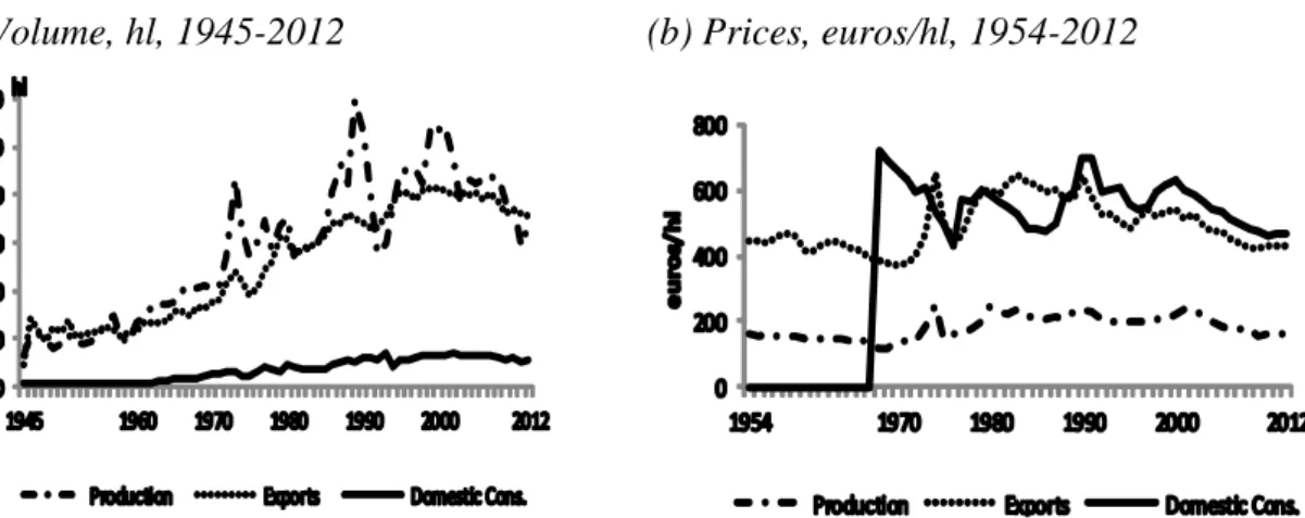
Figure 1 provides a global picture of the data collected. Over the 1945-2012 period the average share of exports in production was 92%, while domestic consumption ac-counted for only 11%. Moreover, production displayed sharper fluctuations than trade (exports and domestic consumption).
(a) Volume, hl, 1945-2012 (b) Prices, euros/hl, 1954-2012
Source: IVDP and the Central Bank of Portugal
Figure 1: Production and trade of Port wine
Real prices in production and trade (exports and domestic market) varied from a minimum value in the early 1970s to a maximum in 1974. The huge difference between trade prices and production prices should also be noted: on average the former typically being triple the latter, that is, the value attributed to the grapes is only one third of the final value of the wine.
For a better understanding of the temporal dynamics, and after transforming each variable into natural logarithms, the series are decomposed in their trend and cycle components, using both the Hodrick-Prescott (HP) filter (Hodrick and Prescott, 1997) and the Baxter-King band-pass (BK) filter (Baxter and King, 1999).9 The results
7 For example, Lütkepohl and Krätzig (2004) and Enders (2010) provide an excellent overview of mod-ern developments in time series methods.
8 For all variables the source is the IVDP (www.ivdp.pt). To convert nominal prices into 2012 real pric-es, the Gross Domestic Product (GDP) deflator was employed, using data from the Portuguese Central Bank (www.bportugal.pt).
9 The literature suggests several techniques for detrending, of which the HP and BK filters are currently the most widely used. See Canova (2007) for a useful survey and discussion.
tained are qualitatively similar. For this reason, and because the BK filter is preferable from a theoretical point of view (Stock and Watson, 1998), for the sake of brevity, in the following analysis the focus will be only on the outputs generated using the BK method.10
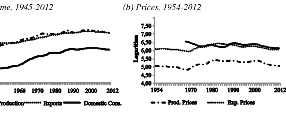
Figure 2 shows that, in volume terms, Port wine production, exports and domestic consumption all display a regular growth pattern. After an initial phase of stagnation or only weak growth until the early 1950s, the three series show a continuous growth trend, with only slight deviations until the end of the 20th century.
(a) Volume, 1945-2012 (b) Prices, 1954-2012
Source: Graphs based on authors’ own calculations
Figure 2: Trends in the production, export and domestic consumption of Port wine
The trend in production prices is similar to that of exports, suggesting that a positive correlation exists between them. After a decrease between 1954 and the end of 1960s, there is an increase in production and export prices until the early 1980s, followed by a negative trend that has persisted until the present 11, interrupted only by a slight upturn in the second half of the nineties. However, the price-trend in domestically-consumed Port wine differs from that of production and exports until the second half of the 1980s: from 1968 to 1976, there is a sharply declining trend, followed by a strong recovery in the second half of the 1980s. Since then, the domestic price trend has followed the nega-tive trend of production- and export-prices.
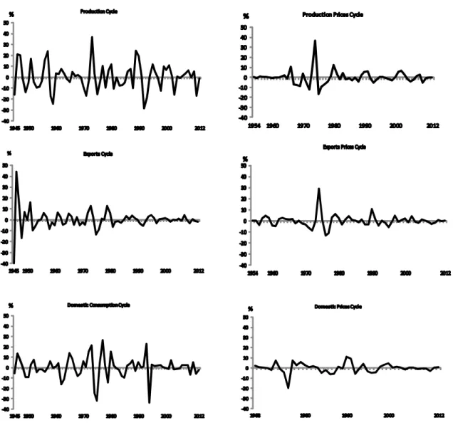
Figure A.1 in Appendix presents the cyclic components of the series, i.e., the devia-tions around the trend12. Production and export cycles of Port wine display similar
10 The results using the HP filter are available from the authors on request. 11
This behaviour seems to anticipate what has happened elsewhere in fine wines. As Candau and Deisting (2014) have noted, wine prices increased globally at a vertiginous rate between 2001 and 2010, but more recently, in the face of stronger competition, price increases have been dampened. In the liquorous wine market (Porto, Sherry, Marsala, Madeira, Samos), Port wine has a dominant posi-tion, Sherry being its main competitor. Based on recent data from the European Union’s international trade data base (COMEX), in 2000, Port wine represented 67% by volume and 78% of the value of the exports of the principal liquorous wines. By 2012, the corresponding proportions had risen to 74% and 84%, respectively, mainly at the expense of second-placed Sherry which, in the same period, with ex-port volume falling from 31% to 16% and value from 21% to 13%.
12 As the values are all in their natural logarithmic form, the units of the cycle correspond to percentage deviations from trend growth paths.
dencies, with phases of growth and contraction clearly synchronized, albeit it is evident a greater magnitude of the production cycles. For both variables, growth peaked in 1946-47, 1951, 1956-57, 1973 and again in 1979-80, although less markedly so for ex-ports. As for contraction, after a sharp decline in 1945, the strongest recessions in Port wine production and exports occurred in 1958-59, 1970-71, 1975 e 1992-93, with pro-duction figures suffering particularly badly. Additionally, the Port wine propro-duction cy-cle also experienced double digit declines in 1998, 2003 and, more recently, in 2011. These cycles do not match those related to domestic consumption, with cyclical fluctua-tions in the latter being more pronounced than those in exports, but smaller than those relating to production.
Port wine price cycles display smaller fluctuations than those related to volume. Price fluctuations were more accentuated in the 1970s, when production and export prices boomed in 1974 (40% and 29% above the trend, respectively) and prices of do-mestically-consumed wine declined sharply in 1976 (20% below the trend). After the 1980s, with the exception of the two-digit growth both in production (in 1980) and in exports and domestic consumption (in 1990), the price cycles displayed only minor variations around the trend.
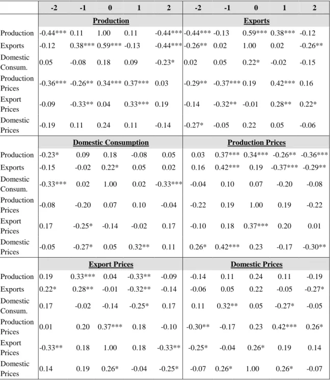
To provide a clearer picture of the degree of synchronization between the cyclical components of the variables related to Port wine, Spearman’s rank correlation coeffi-cients were computed.13 A window of a maximum of 2 years of leads and lags was specified and the highest result of the 5 correlations chosen.14
The results of this exercise (Table A.3 in Appendix) indicate that, as expected, the strongest correlation (0.6) is to be found between production and export cycles, fol-lowed by the moderate contemporaneous relationship between production prices and export prices (0.4) and between domestic prices and export prices (0.3).
Another important outcome is that production price cycles display a moderate corre-lation, with a one-year lag, with those of production, exports and domestic sales (0.4). This is consistent with the fact that prices negotiated between producers and traders are strongly influenced by final market prices.
The results also show a statistically significant albeit weak correlation (0.3), with a one-year lag, between domestic price cycles and the quantities of domestically-consumed Port wine. In contrast, export prices behave in a slightly counter-cyclical manner relative both to the export volumes and domestic consumption, but this correla-tion is weak (-0.3) and characterised by a one year lead.
To verify if Port wine cycles are correlated with Portuguese business cycles, Spear-man correlation coefficients between the cycles displayed by Port wine variables and those of the GDP cycle were computed. The results (Table A.4 in Appendix) do not confirm any strong correlation between the GDP and Port wine cycles.
13 According to Pestana and Gageiro (2005), this coefficient has the advantage of not being sensitive to the possible asymmetry of distributions of the variables or to the presence of outliers, thus not requir-ing the data to be normally distributed.
14 For a more detailed exposition of the interpretation of correlation coefficients see, for example, Sørensen and Whitta-Jacobsen (2010).
4. The Influence of Aging on Price
As previously noted, the potential for fine wine to improve with age implies that it can be viewed, as in the case of other tangible assets, as an alternative to financial in-vestment. However, the results of recent studies aiming to estimate the rate of return on holding wine have produced little consensus: some have concluded that wine is not an attractive investment in comparative terms, while others found wine holding provided a sizeable risk premium.
In general, economic analysts have arrived at their results by using various types of regression-based methods (Fogarty and Sadler, 2014): (a) Hedonic models; (b) Re-peated sales models; (c) Pooled Modes; and (d) Hybrid models. As early as 1979, Krasker, using an adjacent repeated sales model, assessed the holding of red Bordeaux and California Cabernet Sauvignon during the period 1973/74-1976/77, and concluded that the return was lower than that on risk-free assets. In contrast, Jaeger (1981), while using the same estimation method and Krasker’s own dataset, but extending the time frame back a further four years to 1969, found an annual 12% risk premium for storing these two types of wine. Subsequently, Weil (1993), working with a data set of Bor-deaux, Burgundy and Rhône wines held over the 13-year period from 1980 to 1992, discovered that the annual average return was 9.5%, with Bordeaux attaining the highest median return (11%). However, these returns are lower than the returns of NYSE stocks over the same period, that is, the investor would have been better off holding equities.
Burton and Jacobsen (2001) estimated the rate of return on holding red Bordeaux wines for the period 1986-1996, applying the repeated sales regression price index methodology developed by Bailey et al. (1963). Their findings showed an annual nomi-nal rate of return of almost 14% for the sample of 1982, but only 8.3% for that of 1961. But, when comparing the rates of return with the Dow Jones Industrial Average only the 1982 vintage portfolio outperforms this index over the period in question. Fogarty (2006) employed an adjacent period hedonic price regression approach to estimate the return on post-1965 vintage Australian premium wines for the period 1989-2000, and found the return on wine to be higher than that of risk-free assets, but probably not as high as that of an equity portfolio. He also concluded that the quarterly return on more expensive Australian wines was 3.17%, with that of less expensive wines more than a percentage point lower at 1.92%.
Sanning et al. (2008), to analyse returns on red Bordeaux wine, applied models rou-tinely used to forecast equity returns (the Fama - French Three-Factor Model and CAPM - Capital Asset Pricing Model), based on repeat transactions data from monthly auction hammer prices, in the period 1996-2003. Their results indicate that returns on wine averaged up to 0.75% per month above those predicted by these models.
Fogarty (2010), this time using a repeated sales methodology, confirmed his 2006 results for Australian fine wines (i.e. that returns on holding wine are lower than those on standard financial assets), and was able to conclude that wine provides a risk diversi-fication benefit.
Masset and Henderson (2010), using a weighted average of observed prices, were able to show that the return to wine can exceed that of equities, with the cumulative return on holding red Bordeaux wine (145%) in their study period (1996-2007) exceed-ing that registered by the Dow Jones Index (127%). Their results also reveal that, in general, it is vintages of higher quality, along with first growth and second growth
wines, that provide the highest returns. Masset and Weisskopf (2013), from estimates of a repeated sales model, show that returns on wine holding not only exceed those of eq-uities but also bonds and commodities.
Dimson et al. (2014) examined the impact of aging on wine prices and the perfor-mance of wine as a long-term investment using a unique historical database for five long-established Bordeaux wines based on auction and dealer prices. For the period 1900-2012, applying an arithmetic repeat-sales regression, they estimated an annualized return on wine investments (net of insurance and storage costs) of 4.1% in real GBP terms. They further found that, while wine cannot match returns on equities over this extended period, it outperforms government bonds, art and stamps.
Finally, Fogarty and Sandler (2014), using auction data for Australian wines, con-cluded that the estimation method itself has a material impact on the estimated distribu-tion of returns on wine: as with art, the return on wine tends to be overstated when using the repeated sales method, but works satisfactorily with a hedonic model.
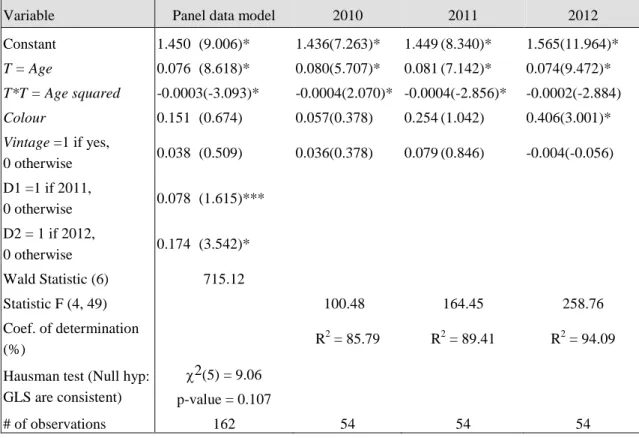
In our case, taking into the account the literature review on the topic, the goal and the availability of data, a hedonic price function was constructed for data relating to the 1934 - 2002 harvests, using 2010, 2011 and 2012 sales prices15, and controlling for col-our and vintage, it was possible to evaluate the influence of ageing on the relative price (logarithm of price). The resultant price function took the following form:
Ln Pt= β0 + β1*T + β2*T2 + β3*Colour + β4*Vintage + µ
where Pt is the trader’s price in the year t; T is the age of the wine (difference between the year of sale and the year of harvest); Colour is expressed as the proportion of white Port wine in total Port production; Vintage is a dummy variable that assumes a value of 1 if the harvest year was classified by IVDP as a vintage year; and µ is the conventional statistical error.
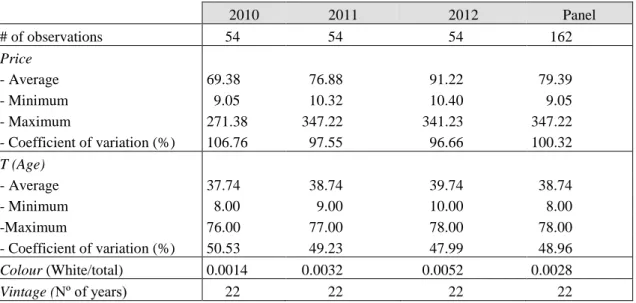
From the data collected, a balanced panel of 162 observations was obtained, with 54 observations for each year (see Table A.5 in appendix). The average price increased from 69.38 euros (2010) to 91.22 euros (2012), averaging 79.39 euros for the panel as a whole. The wine age varies between a minimum of 8 years and a maximum of 78. The Port wine sold is mainly red, and 22 of the harvests between 1934 and 2002 had been declared as vintage by the IVDP.
Table 2 shows the results of the estimations both for each year and for the panel. The outcomes of the Hausman test applied to the panel data confirmed that the existence of a consistent generalized least squares (GLS) model could not be rejected, and were also not favourable to the use of a fixed effects model. Moreover, given the statistical sig-nificance of the values of dummy variables for 2011 and 2012, we concluded that there are differences between the estimations and that, therefore, separate regressions should be made for each year, using robust estimators.
The values of the Wald and R squared statistics indicate that the four regressions are globally significant. Relative to all the independent variables except age, the colour variable turns out to be only statistically significant (with a positive sign) for the year 2012. The non-significance of the vintage variable suggests that the declaration by
15 Prices do not include taxes or subsidies. Based on data provided by IVDP, all prices were subsequently adjusted to reflect 2012 prices, using the appropriate GDP deflator.
IDVP of a year as vintage does not significantly affect prices. Since the variable age is expressed in a quadratic form, its influence on the relative variation of price is given by: β1 +2*β2*T, where β1 is the coefficient associated with T and β2 with T2.
Table 2: Results of the regressions (dependent variable = Ln Price)
Variable Panel data model 2010 2011 2012
Constant 1.450 (9.006)* 1.436(7.263)* 1.449 (8.340)* 1.565(11.964)* T = Age 0.076 (8.618)* 0.080(5.707)* 0.081 (7.142)* 0.074(9.472)* T*T = Age squared -0.0003(-3.093)* -0.0004(2.070)* -0.0004(-2.856)* -0.0002(-2.884) Colour 0.151 (0.674) 0.057(0.378) 0.254 (1.042) 0.406(3.001)* Vintage =1 if yes, 0 otherwise 0.038 (0.509) 0.036(0.378) 0.079 (0.846) -0.004(-0.056) D1 =1 if 2011, 0 otherwise 0.078 (1.615)*** D2 = 1 if 2012, 0 otherwise 0.174 (3.542)* Wald Statistic (6) 715.12 Statistic F (4, 49) 100.48 164.45 258.76 Coef. of determination (%) R 2 = 85.79 R2 = 89.41 R2 = 94.09
Hausman test (Null hyp: GLS are consistent)
2(5) = 9.06 p-value = 0.107
# of observations 162 54 54 54
Source: Authors’ own calculations
Note: Values between brackets (.) are Student t-statistics; *, ** and *** denotes significance at 1%, 5% and 10% levels, respectively.
Table 3 provides the descriptive statistics of the annual price variation rates for each model, and shows the average variation rate to be about 5% although, as the age of the wine increases, the price variation rates decrease, ranging from a maximum of almost 7%, for 8 and 10 year-old Port, to a minimum of 1.8% (in 2010) to 3.3% (in 2012), for a 76 year-old Port. These results are consistent with Dimson et al. (2014), who found a geometric average return of 5.3% for Bordeaux wines harvests between 1900 and 2012. Table 3: Descriptive statistics of the annual rates of variation of prices
Panel data 2010 2011 2012 Annual Variation 0.076-0.0006*T 0.080-0.0006*T 0.081-0.0008*T 0.074-0.0004*T Average 0.050 0.049 0.050 0.053 Min. 0.026 0.018 0.019 0.033 Max. 0.069 0.073 0.074 0.069 Coeff. of variation (%) 24.37 31.22 30.43 18.73
5. Conclusions
Portugal’s Port wine is a globalized product, with the vast bulk of its production ex-ported to a large number of countries around the world. The Port wine filière is heavily regulated, its annual production being set in line with trade forecasts and existing wine stocks.
After World War II the wine industry experienced, in general, until the end of the 20th century, a growth trend that produced positive economic impacts for Port wine traders and grape growers. Similar and clearly synchronized phases of growth and con-traction are displayed both by production and export cycles, albeit with fluctuations in the former more pronounced than in the latter. Furthermore, Port wine price cycles ex-hibited smaller fluctuations than those related to volume, indicating that volatility in the Port wine market is greater for volume than for prices. The last decade has been charac-terised by a downward phase in the cycle of both production and trade, albeit with less pronounced cycles than before.
Our findings suggest, in line with the proposals presented in the Quaternaire Portu-gal/UCP study (2007), that there is an urgent need to strengthen the positioning of Port wine (in general) and its “special categories” (in particular) in contemporary export markets, while at the same time entering new markets where better prices may be of-fered. Since the prices of special categories of Port wine attract higher prices, an appro-priate strategy to compensate for recent declines in export volume and revenues could be to foster the sales of older Port wines.
The results of the application of a hedonic price function allowed us to conclude that the annualized growth in prices is roughly 5%, strongly suggesting that Port wine - given the current returns on other assets - could be considered an interesting financial asset worthy of inclusion in any investor’s portfolio. This conclusion is in line with those presented by Masset and Henderson (2010), Masset and Weisskopf 2013) and Dimson et al. (2014). However, as the annual variation in prices decreases as the age of Port wine increases, compared with investments in other assets, it is not worth holding Port wine for an excessively lengthy period, if the aim of the investor is to maximize annualized returns.
References
Anderson, K., Nelgen, S. (2011). Wine’s Globalization: New Opportunities, New Challenges.
Wine Economics Research Centre Working Paper Nº 0111.
Bailey, M. J., Muth, R. F., Nourse, H. O. (1963). A regression method for real estate price index construction. Journal of the American Statistical Association, 58, 933-942.
Barclays (2012). Profit or pleasure? Exploring the motivations behind treasure trends. Wealth
Insights – Vol. 15.
Baxter, M., King, R. (1999). Measuring Business Cycles: Approximate Band-Pass Filters for Economic Time Series. The Review of Economics and Statistics, 81, 575-593.
Burton, J., Jacobsen, J. P. (2001). The rate of return on wine investment. Economic Inquiry, 39, 337-350.
Candau, F., Deisting, F. (2014). Income and Competition Effects on the World Market for French Wines. AAWE Working Paper Nº 157.
Dimson, E., Rousseau, P. L., Spaenjers, C. (2014). The Price of Wine. Journal of Financial
Economic. Forthcoming. http://dx.doi.org/10.2139/ssrn.2321573.
Enders, Walter (2010). Applied Econometric Time Series. John Wiley & Sons, Inc., New York., 3rd. edition.
Fogarty, J. J. (2006). The return to Australian fine wine. European Review of Agricultural
Eco-nomics, 33, 542-561.
Fogarty, J. J. (2010). Wine investment and portfolio diversification gains. Journal of Wine
Eco-nomics, 5, 119-131.
Fogarty, J. J., Sadler, R. (2014). To save or savor: A Review of Approaches for Measuring Wine as an Investment. Journal of Wine Economics, 9, 225-248.
Hodrick, R., Prescott, E. (1997). Postwar U.S. Business Cycles: An Empirical Investigation.
Journal of Money, Credit and Banking, 29, 1-16.
Jaeger, E. (1981). To save or savor. The rate of return to storing wine: Comment. Journal of
Political Economy, 89, 584-592.
Krasker, W. S. (1979). The rate of return to storing wine. Journal of Political Economy, 87(6), 1363-1367.
Lütkepohl, H., Krätzig, M. (2004). Applied Time Series Econometrics. Cambridge University Press.
Masset, P., Henderson, C. (2010). Wine as an alternative asset class. Journal of Wine
Econom-ics, 5, 87-118.
Masset, P., Weisskopf, J. (2013). Wine as an alternative asset class, in E. Giraud-Heraud and M. Pichery (Eds), Wine Economics: Quantitative Studies and Empirical Applications, New York, Palgrave MacMillan, 173-199.
Pestana, M., Gageiro, J. (2005). Análise de Dados para Ciências Sociais: A
Complementaridade do SPSS. Edições Sílabo, Lisboa, 4th Edition.
Quaternaire Portugal/UCP (2007). Plano Estratégico para os Vinhos com Denominação de
Origem Controlada Douro, Denominação de Origem Porto e Indicação Geográfica Terras Durienses da Região Demarcada do Douro, IVDP, Porto, Portugal.
Rebelo, J., Caldas, J. (2013). The Douro Wine Region: a cluster approach. Journal of Wine
Re-search, 24, 19-37.
Rebelo, J., Correia, L. (2008). Port wine dynamics: production, trade and market structure.
Regional and Sectoral Economic Studies, 8, 99-114.
Rebelo, J., Guedes, A., Lourenço-Gomes, L., Sequeira, M. T. (2013). Balanço de Concretização do Programa de Ação, in Avaliação do Estado de Conservação do Bem ‘Alto Douro
Vinhateiro – Paisagem Cultural Evolutiva Viva’, Vol. 2 – Estudos de Base. Porto: CIBIO
UP/UTAD: B.3-01-B.3-74.
Sanning, L. W., Shaffer, S., Sharratt J. M. (2008). Bordeaux wine as a financial investment.
Journal of Wine Economics, 3, 51-71.
Sørensen, P., Whitta-Jacobsen, H. (2010). Introducing Advanced Macroeconomics: Growth and
Business Cycles. McGraw-Hill, 2nd Edition.
Stock, J., Watson, M.(1998). Business Cycle Fluctuations in U.S. Macroeconomics Time Series.
NBER 6528.
Weil R. L. (1993). Do not invest in wine, at least in the U.S. unless you plan to drink it, and maybe not even then. Paper presented at the 2nd International Conference of the Vineyard Data Quantification Society, Verona, Italy.
Appendix
Table A.1: DDR production in recent years Port wine (hl) Still table wines (hl) DDR produc-tion (hl) Port wine/ DDR prod. (%) Port wine/ Portuguese prod. (%) DDR prod./ Portuguese prod. (%) 2005 845169 873604 1718773 49.17 11.63 23.65 2006 867107 850766 1717873 50.48 11.50 22.78 2007 877405 562786 1440191 60.92 14.45 23.71 2008 871864 502047 1373911 63.46 15.33 24.15 2009 773718 552657 1326375 58.33 13.19 22.61 2010 771777 870483 1642260 46.99 10.80 22.98 2011 590436 729736 1320172 44.72 10.50 23.48 2012 674768 537398 1337280 55.66 10.70 19.21 Total 6272154 5479477 11751631 53.37 12.19 22.85
Source: Authors’ own calculations, based on data published by IVDP and the Vineyard and Wine Insti-tute (Instituto da Vinha e do Vinho – IVV)
Table A.2: Sales of Port wine in recent years
2005 2006 2007 2008 2009 2010 2011 2012 Domestic market - Volume (hl) - Value (103 euro) - Euro/litre 129330 63029 4.87 130860 64224 4.91 128430 61704 4.80 125100 59578 4.76 110160 51874 4.71 120906 55327 4.58 106607 50321 4.72 110339 52104 4.72 Exports - Volume (hl) - Value (103 euro) - Euro/litre 807750 341930 4.23 785250 331685 4.22 814050 342550 4.21 767070 316222 4.12 725940 300266 4.14 741604 315474 4.25 718624 305592 4.25 715273 308282 4.31 Total - Volume (hl) - Value (103 euro) - Euro/litre 937080 404959 4.32 916110 395909 4.32 942480 404254 4.29 892170 375800 4.21 836100 352100 4.21 862511 370801 4.30 825230 355912 4.31 825612 360386 4.37 Source: IVDP
Source: Graphs based on authors’ own calculations
Table A.3: Coefficients of correlation between the cycles of variables -2 -1 0 1 2 -2 -1 0 1 2 Production Exports Production -0.44*** 0.11 1.00 0.11 -0.44*** -0.44*** -0.13 0.59*** 0.38*** -0.12 Exports -0.12 0.38*** 0.59*** -0.13 -0.44*** -0.26** 0.02 1.00 0.02 -0.26** Domestic Consum. 0.05 -0.08 0.18 0.09 -0.23* 0.02 0.05 0.22* -0.02 -0.15 Production Prices -0.36*** -0.26** 0.34*** 0.37*** 0.03 -0.29** -0.37*** 0.19 0.42*** 0.16 Export Prices -0.09 -0.33** 0.04 0.33*** 0.19 -0.14 -0.32** -0.01 0.28** 0.22* Domestic Prices -0.19 0.11 0.24 0.11 -0.14 -0.27* -0.05 0.22 0.05 -0.06
Domestic Consumption Production Prices
Production -0.23* 0.09 0.18 -0.08 0.05 0.03 0.37*** 0.34*** -0.26** -0.36*** Exports -0.15 -0.02 0.22* 0.05 0.02 0.16 0.42*** 0.19 -0.37*** -0.29** Domestic Consum. -0.33*** 0.02 1.00 0.02 -0.33*** -0.04 0.10 0.07 -0.20 -0.08 Production Prices -0.08 -0.20 0.07 0.10 -0.04 -0.22 0.19 1.00 0.19 -0.22 Export Prices 0.17 -0.25* -0.14 -0.02 0.17 -0.10 0.18 0.37*** 0.20 0.01 Domestic Prices -0.05 -0.27* 0.05 0.32** 0.11 0.26* 0.42*** 0.23 -0.17 -0.30**
Export Prices Domestic Prices
Production 0.19 0.33*** 0.04 -0.33** -0.09 -0.14 0.11 0.24 0.11 -0.19 Exports 0.22* 0.28** -0.01 -0.32** -0.14 -0.06 0.05 0.22 -0.05 -0.27* Domestic Consum. 0.17 -0.02 -0.14 -0.25* 0.17 0.11 0.32** 0.05 -0.27* -0.05 Production Prices 0.01 0.20 0.37*** 0.18 -0.10 -0.30** -0.17 0.23 0.42*** 0.26* Export Prices -0.33** 0.18 1.00 0.18 -0.33** -0.25* -0.04 0.26* 0.19 0.14 Domestic Prices 0.14 0.19 0.26* -0.04 -0.25* -0.07 0.26* 1.00 0.26* -0.07
Source: Authors’ own calculations
Table A.4: Coefficients of correlation between the GDP cycle and the cycle of Port wine variables -2 -1 0 1 2 Production 0.07 0.20 0.20 -0.09 -0.15 Exports 0.02 0.26** 0.27** -0.15 -0.35*** Domestic Consum. 0.29** 0.37*** 0.19 -0.16 -0.31** Production Prices -0.07 0.15 0.43*** 0.32** 0.06 Export Prices -0.20 0.02 0.34*** 0.21 -0.06 Domestic Prices 0.25* 0.41*** 0.36*** 0.22 -0.14
Source: Authors’ own calculations
Note: *, ** and *** indicate significance at the 10%, 5% and 1% levels, respectively; the GDP variable, at constant 2012 prices for the 1955-2012 period, was constructed using data from the Central Bank of Portugal and EUROSTAT.
Table A.5: Descriptive statistics of price, age, colour and vintage years
2010 2011 2012 Panel # of observations 54 54 54 162 Price - Average 69.38 76.88 91.22 79.39 - Minimum 9.05 10.32 10.40 9.05 - Maximum 271.38 347.22 341.23 347.22 - Coefficient of variation (%) 106.76 97.55 96.66 100.32 T (Age) - Average 37.74 38.74 39.74 38.74 - Minimum 8.00 9.00 10.00 8.00 -Maximum 76.00 77.00 78.00 78.00 - Coefficient of variation (%) 50.53 49.23 47.99 48.96 Colour (White/total) 0.0014 0.0032 0.0052 0.0028 Vintage (Nº of years) 22 22 22 22