Role of fractures in weathering of solid rocks: narrowing the gap between laboratory and field weathering rates

ROLE OF FRACTURES IN WEATHERING OF SOLID ROCKS: NARROWING THE GAP BETWEEN LABORATORY AND FIELD WEATHERING RATES

by

Fernando A. L. Pacheco1,2 and Ana M. P. Alencoão1,3

1

Geology Department, Trás-os-Montes and Alto Douro University, 5000 Vila Real, Portugal & Centre for Geophysics, Coimbra University, Coimbra, Portugal.

2

[email protected] 3

ABSTRACT

A weathering study of a fractured environment composed of granites and metasediments was conducted in Trás-os-Montes and Alto Douro (north of Portugal) and covered the hydrographic basin of Sordo river. Within the basin, a number of perennial springs were monitored for discharge rate, which allowed for the estimation of annual recharges. A small area of the basin was characterized for parameters such as hydraulic conductivity and effective porosity, which, in combination with the previously calculated recharges, allowed for the calculation of a fracture surface area. The monitored springs were also sampled and analyzed for major inorganic compounds, and using a mole balance model the chemistry of the water samples was explained by weathering to kaolinite of albiteoligoclase plus biotite (granites) or of albite plus chlorite (metasediments). The number of moles of dissolved primary minerals (e.g. albite) could be calculated using this method. These mass transfers were then multiplied by the spring’s median discharge rate and divided by the fracture surface area to obtain a weathering rate. Another weathering rate was determined, but using a BET surface area as normalizing factor. Comparing both rates with a representative record of laboratory as well as of field-based weathering rates, it has been noted that rates normalized by the BET were, as expected, similar to commonly reported field-based rates, whereas rates normalized by the fracture surface area were unexpectedly relatively close to laboratory rates (one order of magnitude smaller). The monitored springs are of the fracture artesian type, which means that water emerging at the spring site flowed preferentially through joints and fractures and that weathering took place predominantly at their walls. Consequently, it was concluded that the most realistic weathering rates are those normalized by the fracture surface area, and as a corollary that the gap between laboratory and field weathering rates might not be as wide as usually is reported to be.

INTRODUCTION

Do mineral weathering rates differ significantly between the laboratory and the field environments? The most recent attempt on the reconciling between laboratory and field-based weathering rates is the work by White and Brantley (2003). In this work the focus was put on the effect that time has on the weathering rates of silicate minerals, and the general conclusions were that weathering rates decrease with weathering duration according to a power function. Notwithstanding this function has been derived from a considerably large record of laboratory and field-based rates, a crucial question to be put is if the large apparent decrease in weathering rates with time are not artifacts based on normalization using gas sorption isotherms (BET surface areas) which overestimate actual increases in the reactive surface area with time. For instance, it has been proposed by Gautier et al. (2001) that much of the measured increase in BET surface area during weathering consisted of increases in essentially unreactive walls of etch pits that contributed negligibly to mineral dissolution, and other scenarios that decouple the reactive surface area from the measured physical surface area were addressed by White and Peterson (1990), Drever and Clow (1995) and Brantley et al. (1999). But there is a scenario not yet studied systematically that can be stated as follows: is it realistic a normalization of weathering rates based on the BET surface area of disaggregated rock samples (usual approach) when in environments like granites and metasediments most of the flow is through a network of joints and fractures? The problem is that in the first case it is assumed that water interacts with all grains in the sample, which means a larger but eventually unreal reactive surface area, whereas in the second case it is implicit that water contacts essentially with grains facing the fracture walls, which implies a much smaller but eventually true reactive surface area. The purpose of this paper is to work on a scenario like this. To that end, we first settled on a formula

that describes more realistically the surface area of a fractured medium, and then verified how weathering rates normalized by this area compare with commonly reported laboratory and field-based rates.

STUDY AREA

The hydrographic basin of Sordo river is located in Trás-os-Montes and Alto Douro (north of Portugal, near Vila Real) and covers an area of approximately 51.2 km2 (Figure 1).

Geology, Mineralogy and Petrology

The geology of Sordo river basin is characterized by Paleozoic metasediments that were intruded by Hercynian granites and covered in the valleys by alluvial deposits (Figure 1). The oldest terrains are dated from the Cambrian and are composed essentially of alternating phyllites and greywackes. The Ordovician rocks crop out at the Northwest border of the basin and are made predominantly of a conglomerate overlain by alternating quartzites and phyllites The granites are syn-tectonic with respect to the third phase of the Hercynian orogeny and are two-mica medium to coarse grained granites. The contact between granites and metasediments is characterized by an abundance of aplitic dykes, trending towards the Northwest, which acted as a barrier to drainage promoting a selective accumulation of alluvial deposits on top of the Cambrian rocks. The rock massifs are fractured intensely by a set striking to NESW till NNESSW, sometimes filled with quartz (mostly), pegmatites and aplites, and by a conjugate set striking to NWSE (Sousa, 1982; Pereira, 1989, Matos, 1991), usually not filled.

This study is focused on springs emerging from Cambrian metasediments and granites. The mineralogical composition of the metasediments is characterized by an assemblage with quartz, albite, chlorite and muscovite. The granites are composed mainly of quartz, K-feldspar, plagioclase (albiteoligoclase), biotite and muscovite (Sousa, 1982; Matos, 1991). There is no information on the chemical composition of minerals composing the local metasediments, but reliable information on very similar rocks could be gathered from Pacheco and Van der Weijden (2002). The chemical composition of muscovite and biotite was determined for the granites by Matos (1991). The structural formulas of the rock forming minerals are depicted in Table 1. The mineral abundances (last two columns) were determined by the Balance of Cation Proportions (Pacheco and Van der Weijden, 2002).

Soils

The hydrographic basin of Sordo river is covered by leptosols (dominant type), fluvisols (in the stream valleys) and some anthrosols (Figure 2). The cartography was made by Agroconsultores & Coba (1991) who characterized soil types for thickness as follows: < 25 cm for the leptosols and around 60 cm for the other types. This study is focused on springs emerging from the rather thin leptosols (mostly) meaning that water-mineral interactions took place essentially at the uppermost horizons of the fractured rock. The clay fraction of the soils is composed of kaolinite with small amounts of vermiculite (Silva, 1983).

Recharge to Springs

From May 2002 till September 2002 a number of springs (161) were mapped in the Sordo river hydrographic basin. From July 2002 till October 2003 a small subset of these springs (31) were monitored monthly for discharge rate. Spring sites were plotted over a map of ‘fracture’ densities quantified from lineaments observed in aerial photographs (Figure 3). Springs are located preferably where ‘fracture’ densities are high, suggesting that they are of fracture artesian nature. The dominance of fracture springs in massifs of crystalline rocks has been noted before, and discussed in detail by Pacheco and Alencoão (2002) in a study involving over 1500 springs and 640 km2 area.

The measured discharge rates (Table 2) were used to estimate the recharge associated with each spring. The method used is described elsewhere (Domenico and Schwartz, 1990) and may be summarized as follows: if Qf (m3/s) is the base flow at the end of a recession and Qi (m3/s) the

base flow at the beginning of the next recession, then the recharge taking place between the two periods is:





where R (m3) is the recharge and t1 (s) the time corresponding to a log cycle of discharge. The

results obtained for all the samples are listed in Table 2 (last column) from which a median value of 4711 m3 could be determined. An application of the estimation procedure is illustrated in Figure 4 for spring Nr 13. The minimum base flow of the early recession is Qf = 0.005 l/s and the

maximum of the subsequent recession Qi = 0.160 l/s. The time corresponding to a log cycle of

Hydraulic Conductivity and Effective Porosity of a Fractured Medium

The hydraulic conductivity and effective porosity of fractured phyllites were estimated by a finite differences method. The method is standing on two forms of the general rate equation (in Domenico and Schwartz, 1990):

s B t       (2) where t 

 _{is a flux (temporal variation of ),} s 

 _{is a gradient (spatial variation of ) and B is a}

conductance (a property of the medium). The Darcy’s law:

s h K t h      (3)

is one of these forms, where the flux         t h

is the vertical component of the specific discharge,

the gradient         s h

is the slope of the water table and the conductance (K) is the hydraulic

conductivity of the fractured medium. The other form of the general rate law is the advection equation describing mass transport in the absence of dispersion or diffusion:

s C v t C      (4)

where C means concentration of a dissolved mass and

s h n K v  

 means velocity of water in the

mean direction of flow; variable n is the effective porosity of the fractured medium. Electrical conductivity of water (Ec) is a proxy to the sum of dissolved solids and for that reason will be used as C.

In order to calculate K and n, a number of dug wells in the study area must first be monitored for hydraulic head (h) and Ec during a certain period of time, and then the measured h and Ec values interpolated over a grid of regularly spaced nodes with a distance y between rows and x between columns. Providing that y, x and t are small, the following equations apply to each node in the grid:

1 2 1 , 2 , t t t t t i t i i i            (5a) 2 , , 2 , , 2 2 _                      y x s s S i N i W i E i i i       (5b)

where i,t is the score of  (h or Ec) at node i given the time t, and N(S,E,W) are the scores of  at

nodes located one row or one column to the North, South, East or West of node i. Based on grids constructed by Equations 5a,b, new grids containing the values of K, v and n are computed by the following equalities: s h t h K      (6a) s Ec t Ec v      (6b) s h v K n    (6c)

where || means absolute value of .

In the Sordo river hydrographic basin, 10 dug wells were monitored monthly for h and Ec from February 2003 till November 2003. The location of wells is given in Figure 5 and the values of h and Ec listed in Table 3. All wells were dug in the fractured phyllites till several meters deep, and as expected most wells are in areas where ‘fracture’ densities are relatively high (Figure 5).

The values of K and n were estimated by the finite differences method described above. First, the h and Ec values of each month (Table 3) were interpolated over regular grids with y =5 m and x =5 m, while t was set to 30 days. Second, for each node in those grids, temporal and spatial gradients were calculated by Equations 5a and 5b, K and n by Equations 6a and 6b. Third, median and inter-quartile values of K and n were determined that represent the entire shaded area of Figure 5. The calculated medians and inter-quartiles are shown in Figure 6 and were combined with median depths of the water table. The water table lowers down from about 1 m depth in early Spring and mid Fall to approximately 3 m depth in late Summer. The drawdown of the water table is followed by a decrease in the medians of K and n, at least in the period going from June (K = 6.39×106 m/s, n = 3.6%) to September (K= 1.12×106, n = 0.3%). The estimated K and n medians are representative of a fractured phyllite, not of a disaggregated rock or a soil. The decrease in their values from Spring to Summer indicates that as the water table goes down groundwater flows through more compact and impermeable sectors of the metassediment. The ratios between upper quartiles (75% of the population) and medians are just 20.4 for K and 20.6 for n, meaning that spatial heterogeneity is just moderate. Given the lack of long and detailed records of h and Ec, no attempt was made to inspect the nature of heterogeneity and the possible importance of fractal processing (Kirchner et al., 2000, 2001; Neal, 2002).

It should be noted that we wanted to monitor h and Ec of granite well water, but that was not possible given the very few number of wells that were mapped in granite outcrops. For that reason, the estimated K and n medians will be used as references throughout the reminder of this paper.

WATER SAMPLING AND ANALYTICAL RESULTS

In September 2002, the monitored springs (Figure 3) have been sampled and analyzed for major inorganic compounds. At the sampling site, temperature (T), electrical conductivity (Ec) and pH were measured using WTW (models LF 320 and PH 320) portable meters. The samples used for chemical analyses were stored unacidified in 125 ml polyethylene flasks. Major cations and silicon were determined by ICP-MS using a Perkin Elmer ELAN 6000 spectrometer, bicarbonate by titration to pH 4.5 using 0.02 N H2SO4, chloride, sulfate and nitrate by Ion Chromatography

using a DIONEX DX-120 System. The analytical results are listed in Table 4. The median deviation from charge balance (column under heading Err) is 5.1%, which is acceptable for dilute waters.

WEATHERING AND SPRING WATER CHEMISTRY

From Soil Water to Spring Water

The parent of spring water is soil water. Following respiration or oxidation of organic matter, soil water dissolves CO2 that subsequently is used in weathering reactions. The pH of soil water

(pHin) can be estimated from the bicarbonate concentration and pH of spring water (pH), as

follows (Apello and Postma, 1993):









where PCO2 (atm) is the partial pressure of CO2 and [HCO3-] is the concentration of bicarbonate

in the spring. Estimates of PCO2 and pHin are listed in Table 4 and show that, due to the effects of

respiration and oxidation of organic matter log(PCO2) = 1.60.5, i.e. spring water is far from

being in equilibrium with the atmosphere (in such case log(PCO2) would be 3.5), and that before

flowing through the rock fractures the pH of underground water ranged from 4.3 to 5.1.

Soil pH and the initial concentrations of soil water solutes, in particular of bicarbonate, are raised by interaction between infiltrating water and minerals, the magnitude of such increase being dependent on the residence time. A regression between pH and [HCO3] indicates that

weathering imprints a major signature on the chemistry of springs, and in complement that there is an ample range of residence times. In our case we found that

[HCO3] = 7.8pH  32.6, valid for 4.5 < pH < 6.7, with r2

= 0.5 (8)

Water Mineral Interactions

Not all the minerals present in the various rocks of the study area are important as weathering reactants. The weathering products (essentially kaolinite) are derived mainly from albiteoligoclase (An0An20) plus biotite in the granites or from albite (An0An10) plus chlorite

in the metasediments. The reactions describing the alteration of plagioclase, biotite and chlorite into kaolinite are listed in Table 5.

The number of moles of weathered plagioclase, biotite and chlorite producing a certain spring water composition may be determined by mole balance models. We used the SiB algorithm, a method introduced by Pacheco and Van der Weijden (1996), that was extended by Pacheco et al.

(1999), Pacheco and Van der Weijden (2002) and Van der Weijden and Pacheco (2003), and that comprehends a set of mole balance and charge balance equations of the form:

Mole balance equations 

 

   

q j ij  



 , with i=1,q2 (9a)

Charge balance equation  z

 

 



  

q l l l       



 q1, q2 and q3 are the number of primary minerals involved in the weathering process (albiteoligoclase plus biotite or albite plus chlorite in the present case), the number of inorganic compounds that usually are released from weathering reactions (in total six compounds  Na+, K+, Mg2+, Ca2+, HCO3 and H4SiO4), and the number of the latter

compounds that usually are also derived from pollution (the four major cations);

 t and p mean total and derived from pollution, respectively. The expected sources of pollution are manures, commercial fertilizers and domestic and/or industrial effluents.  Y represents a dissolved compound;

 M represents a mineral;

 Cl, SO42 and NO3 are the abbreviations for chloride, sulfate and nitrate, the major

dissolved anions assumed to represent exclusively anthropogenic plus atmospheric inputs;

 Square brackets ([]) denote number of moles of a dissolved compound or a dissolved mineral;

 ij is the ratio between the stoichiometric coefficients of dissolved compound i and

 ij[Mj]=[Yi]rj, where [Yi]rj is the number of moles of dissolved compound i derived from

reaction of Mj moles of mineral j;

 zl is the charge of cation l;

The number of equations in set 9a,b is seven. The unknowns of the system are the [M] and the [Y]p variables, in total q1+q3. The SiB algorithm uses the Singular Value Decomposition procedure as described in Press et al. (1989) to solve the set of equations because this procedure can handle efficiently (through least squares or minimizing procedures) the cases where the set is undetermined (q1+q3 > 7) or overdetermined (q1+q3 < 7). In the present case set 9a,b is overdetermined (q1+q3 = 6).

The number of moles of dissolved plagioclase, biotite an chlorite were determined using Equations 9a,b, with concentrations taken from Table 4 and reaction coefficients taken from Table 5. The results are listed in Table 6 (columns 35). The SiB algorithm could explain the chemical composition of 28 out of the 31 springs. In all cases but 3 the plagioclase type fitting best to the weathering model was albite (0  x  0.1). A major portion of the natural contribution to water chemistry is attributed to weathering of plagioclase (86.5%), with the remainder being assigned evenly to alteration of biotite (5.3%) and chlorite (8.2%). These results agree with widely accepted sequences of weathering (e.g. Goldish, 1938; Berner, 1971).

REACTIVE SURFACE AREAS AND MINERAL WEATHERING RATES

Reactive Surface Areas

A mineral weathering rate obtained from a laboratory experiment or field study is frequently normalized by a physical surface area (e.g. BET surface area), assumed to be the reactive surface area. For a sample with mass M (kg) and particles with specific surface area SM (m2/kg) the area

available for reaction (AM in m2) is usually reported to be:

AM = M SM (10)

Application of Equation 10 assumes that water interacts with all grains of mineral M in the sample, but in the field this may occur solely when the weathering environment is a soil, saprolite or unconsolidated sediment, not when water percolates through a fractured rock.

In a fractured rock, flow is promoted when a critical degree of connectivity between fractures is attained (percolation threshold), i.e. flow is limited to the so called fault zone aquifers (e.g. Pacheco, 2002) or preferential flow paths. For example, should a percolation threshold of 10 kilometers of fractures per square kilometer of area be assumed for Figure 5 and the preferential flow paths would be represented by the shaded areas. On the other hand the area available for weathering reactions within a preferential flow path is restricted essentially to minerals facing the fracture walls. The combined effect of limited flow circuits and restricted assess to mineral surfaces is a reactive area that can be orders of magnitude smaller than that calculated by Equation 10. And the consequence of a misuse of this equation is the underestimation of field weathering rates.

To prevent miscalculation of weathering rates, the estimation of a reactive surface area in this study is hinged on the concept of equivalent hydraulic conductivity proposed by Snow (1968). For a set of planar fractures the hydraulic conductivity (K) of a fractured massif is given by:

w wgNb K   12 3  (11)

where wkg/m3andw(kg/(s.m)) are the specific weight and dynamic viscosity of water,

respectively, g (9.81 m/s2) is the acceleration of gravity, b (m) is the fracture opening and N (1/m) is the number of fractures per unit distance across a square meter of rock surface. The physical properties wandw aredependent on water temperature. We adopted w = 999.1

kg/m3 and w = 1.14  103 kg/(s.m), which are representative of T = 15 ºC. In the natural world,

however, crystalline rock masses are usually cut by several sets of planar discontinuities and for that reason N is better equated to the number of fractures per unit distance across a cubic meter of rock.

In Equation 11, Nb3/12 is the intrinsic permeability of the fractured medium (k) and Nb its planar porosity (n). Replacing Nb by n in that equation and rearranging gives for N:

K gn N w w   12 3  (12)

which in turn gives for AM:

K gn R N n R N V A A w w M M M M M       12 2 2 2             (13)

where A is the fracture surface area and M the proportion of mineral M in the rock (M  A is the

fracture surface area of mineral M); V is the volume of rock with effective porosity n that stored R cubic meters of infiltrated water; and constant 2 means that for each fracture there are usually

two reactive surfaces (the two fracture walls). We note that AM, as calculated by Equation 13, is

independent of phenomena such as partial wetting, because V is indexed to recharge. However, Equation 13 assumes that fracture walls have the same composition as the rocks in which they occur. This assumption does not hold when fractures had been filled forming dykes, so, inherently, we are assuming that for instance quartz, pegmatite or aplite veins are present in the rock massifs in a negligible proportion.

The medians of R, K and n are 4711 m3 (Table 2), 2.77106 m/s and 0.014 (Figure 6), respectively. Replacing these values in Equation 13 and considering that plagioclase (essentially albite) abundance in the granites is 24.5% and that in the metasediments is 10.5% (Table 1), we can derive that AAb = 1.39108 and 5.95107 m2, respectively. It should be noted that these

values are significantly smaller than counterparts estimated by Equation 10. Indeed, making a note that the mass of albite (Ab) would be given by:

Ab Ab Ab n R_{ }   (14)

where Ab is the specific weight of albite (2620 kg/m3), and that a median BET SAb = 80 m2/kg is

reported in Blum (1994), then the median reactive surface areas of albite would approach 1.731010

m2 in the granites and 7.41109 m2 in the metasediments. The ratio between the former and these areas is 8.04103 meaning that a weathering rate standing on the latter areas would be underestimated by 2 to 3 orders of magnitude. Similar results would be obtained for biotite or chlorite. In the case of biotite, for example, the fracture-based reactive surface area is

2.15107

m2, while the BET-based area is 6.381010 m2 if we adopt Bt = 9416 kg/m3, given the

composition of biotite (Table 1), and SBt = 530 m2/kg (Sverdrup, 1990). The ratio between the

these areas is 3.37104 meaning that in these case a weathering rate standing on the latter areas would be underestimated by 3 to 4 orders of magnitude.

Mineral Weathering Rates

The weathering rate of a mineral M (WM) is given by:

 

where Qmed is the spring’s median discharge rate, [M] is the number of moles of M that dissolved

during weathering and AM is the fracture surface area of M. The [M] values of Sordo’s springs

are depicted in columns 35 of Table 6, the corresponding median Q values were determined from data in Table 2 and are listed in column 6, the A values were derived from Equation 13 and are shown in column 7, and the weathering rates of plagioclase, biotite and chlorite were computed by Equation 15 and their logarithms are listed in columns 810. Plagioclase weathering rates vary within less than one order of magnitude (log WPl = 12.7±0.3), the same

happening with the rates of chlorite (log WCh = 13.8±0.3). For biotite the standard range of rate

values is within a bit more than one order of magnitude (log WBt = 13.4±0.6).

RECONCILING LABORATORY AND FIELD WEATHERING RATES

White and Brantley (2003) compiled from the literature a considerably large record of plagioclase and biotite weathering rates that were measured from laboratory experiments or

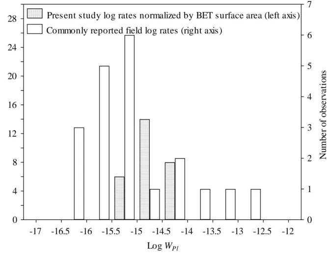
estimated in the field. In all cases the rates were already or have been normalized by the BET surface area. The distributions of plagioclase log rates are represented in Figures 7a and 7b by the white histograms. In both cases weathering rates span several orders of magnitude, a variation that essentially has been attributed to a time effect. This time argument has also been used to justify the usual reports that, on average, field rates are several orders of magnitude smaller than laboratory rates.

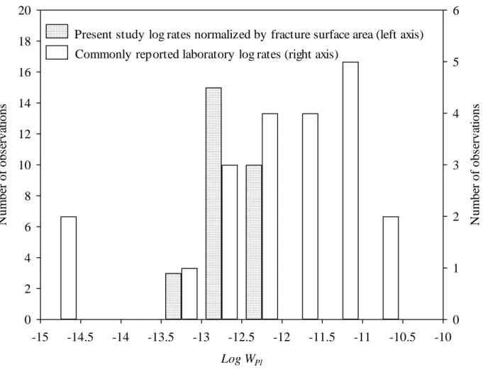
In view of our own results, the strongest argument that helps explaining the huge discrepancy between laboratory and field weathering rates is the underestimation of field rates due to BET normalization. The rationale for plagioclase is as follows: (1) on one hand, the distribution of present study log rates, but expressed as BET log rates (Table 6 values reduced by log(8.04103

)), matches the highest frequencies of published field rates (compare the white and dotted histograms of Figure 7a), meaning that our results are consistent with results by other workers when the assumption made about the reactive surface area is identical; (2) on the other hand, it was demonstrated for fractured rocks that a realistic reactive surface area is represented by the fracture surface area (Equation 13), and rates normalized by this area (Table 6 values) are solely one order of magnitude smaller than laboratory rates (compare the white and dotted histograms of Figure 7b). Thus, if a real discrepancy exists between field and laboratory weathering rates, this is probably represented by a factor of 10 or so difference, not by a factor of 1000 or more difference.

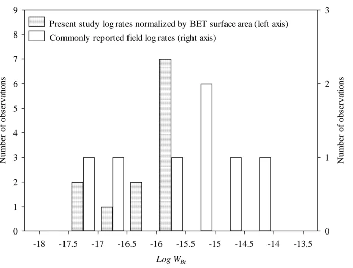
The discussion made for plagioclase can be transposed to biotite because present study weathering rates normalized by the BET area (Table 6 values reduced by log(3.37104)) are comparable to reported field weathering rates (Figure 8a), and simultaneously present study

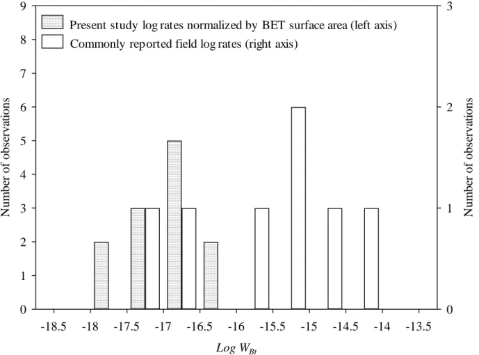
weathering rates normalized by the fracture surface area are on average one order of magnitude smaller than reported laboratory rates (Figure 8b).

CONCLUSIONS

In this study of weathering of solid rocks, it has been demonstrated that the gap between laboratory and field weathering rates can be narrowed if rates are normalized by a fracture surface area derived from field-estimated hydraulic parameters (hydraulic conductivity, effective porosity) instead of a BET surface area measured over samples of disaggregated rock. We believe our approach is correct because in geological environments such as granites and metasediments, groundwater flows essentially through joints and fractures and minerals weather predominantly at joint and fracture walls.

ACKNOWLEDGEMENTS

REFERENCES

Agroconsultores & Coba, 1991. Carta de solos, carta do uso actual da terra e carta de aptidão da terra do nordeste de Portugal. Technical Report, Trás-os-Montes e Alto Douro University, Vila Real, 311 pp.

Berner, R.M., 1971. Principles of chemical sedimentology. McGraw-Hill, New York, 240 pp.

Blum, A.E., 1994. Feldspars in weathering. In: Parsons I. (Ed.), Feldspars and Their Reactions. Kluwer Academic Publishers, Dordrecht, pp. 595630.

Brantley, S.L., White, A.F., Hodson, M.E., 1999. Surface areas of primary silicate minerals. In: Jamtveit, B, Meakin, P. (Eds.), Growth, Dissolution and Pattern Formation in Geosystems. Kluwer Academic Publishing, Dordrecht, pp. 291326.

Domenico, P.A., Schwartz, F.W., 1990. Physical and chemical hydrogeology. John Wiley & Sons Inc., New York, 824 pp.

Drever, J.I., Clow, D.W., 1995. Weathering rates in catchments. In: White A.F., Brantley, S.L. (Eds.), Chemical Weathering Rates of Silicate Minerals. Mineral Soc. Amer, 31: 463481.

Gautier, J.M., Oelkas, E.H., Schott, J., 2001. Are quartz dissolution rates proportional to B.E.T. surface areas? Geochim Cosmochim Acta, 65: 0591070.

Kirchner, J.W., Feng, X., Neal, C. (2000) Fractal stream chemistry and its implications for contaminant transport in catchments. Nature, 403: 524527.

Kirchner, J.W., Feng, X., Neal, C. (2000). Catchment-scale advection and dispersion as a mechanism for fractal scaling in stream tracer concentrations. Journal of Hydrology, 254: 82101.

Matos, A.M., 1991. A geologia da região de Vila Real. PhD Thesis, Trás-os-Montes and Alto Douro University, Vila Real, 312 pp.

Neal, C. (2002). From determinisn to fractal processing, structural uncertainty, and the need for continued long-term monitoring of the environment: the case of acidification. Hydrological processes, 16: 24812484.

Pacheco, F.A.L., 2002. Response to pumping of wells in sloping fault zone aquifers. Journal of Hydrology, 259: 116135.

Pacheco, F.A.L., Alencoão, A.M.P., 2002. Occurrence of springs in massifs of crystalline rocks, northern Portugal. Hydrogeology Journal, 10: 239253.

Pacheco, F.A.L., Van der Weijden, C.H., 1996. Contributions of water-rock interactions to the composition of groundwater in areas with sizeable anthropogenic input. A case study of the waters of the Fundão area, central Portugal. Water Resour Res, 32: 35533570.

Pacheco, F.A.L., Van der Weijden, C.H., 2002. Mineral weathering rates calculated from spring water data. A case study in an area with intensive agriculture, the Morais massif, NE Portugal. Appl Geochem, 17: 583603.

Pacheco, F.A.L., Sousa Oliveira, A., Van der Weijden, A.J., Van der Weijden, C.H., 1999. Weathering, biomass production and groundwater chemistry in an area of dominant anthropogenic influence, the ChavesVila Pouca de Aguiar region, north of Portugal. Water Air Soil Pollut, 115: 481512.

Pereira, E., 1989. Notícia explicativa da folha 10-A (Celorico de Basto). Direcção Geral de Geologia e Minas, Serviços Geológicos de Portugal, 53 pp.

Press, W.H., Flannery, B.P., Teukolsky, S.A., Vetterling, W.T., 1989. Numerical Recipes in Pascal, Cambridge University Press, Cambridge, 759 pp.

Silva, J.M.V., 1983. Estudo mineralógico da argila e do limo de solos derivados de granitos, xistos e rochas básicas da região de Trás-os-Montes. Garcia de Orta, Ser. Est. Agron., v. 10(12), pp. 2736.

Snow, D.T., 1968. Rock fracture spacings, openings, and porosities. Journal of Soil Mechanics, 94: 7391.

Sousa, M.B., 1982. Litoestratigrafia e estrutura do “Complexo Xisto-Grauváquico ante-Ordovícico” - Grupo do Douro (Nordeste de Portugal). PhD Thesis, Coimbra University, 223 pp.

Sverdrup, H.U. (1990). The kinetics of base cation release due to chemical weathering. Lund University Press, Lund, Sweden, 246 pp.

Van der Weijden, C.H., Pacheco, F.A.L., 2003. Hydrochemistry, weathering and weathering rates on Madeira island. Journal of Hydrology, 283: 122145.

White, A.F., Brantley, S.L., 2003. The effect of time on the weathering of silicate minerals: why do weathering rates differ in the laboratory and field?. Chem Geol, 202(34): 479506.

White, A.F., Peterson, M.L., 1990. The role of surface area characterization in geochemical models. In: Melchior, R.L., Bassett, R. (Eds.), Chemical Modeling of Aqueous Systems II. Amer. Chem. Soc. Symp. Ser., 416: 461475.

TABLE LEGENDS

Table 1 – Mineralogical composition of the Cambrian metasediments and of the Hercynian granites. Structural formulas of chlorite and of metasediments’ muscovite were compiled from Pacheco and Van der Weijden (2002); of biotite and of granites’ muscovite from Matos (1991). Abundances were determined by the Balance of Cation Proportions (Pacheco and Van der Weijden, 2002). Variable x is the anorthite content of plagioclase; for the granites, 0  x  0.2 (plagioclase is albiteoligoclase) and for the metasediments 0  x  0.1 (plagioclase is albite).

Table 2 – Hydrological parameters of the monitored springs (location in Figure 3). Monitoring period: July 2002October 2003. Symbols: Nr  spring’s identification code; M and P  Hayford-Gauss coordinates; t – time passed since the monitoring campaign has started. Q  measured discharge rate; R  recharge between recession periods as determined by Equation 1.

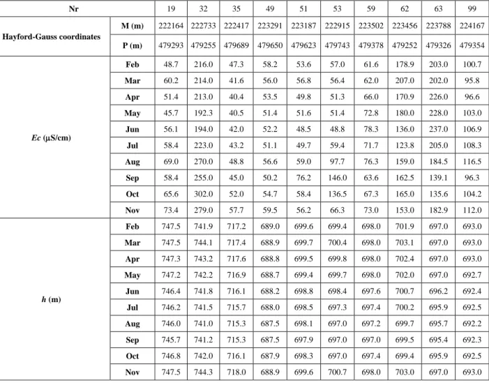
Table 3 – Hydraulic head (h) and electrical conductivity (Ec) data of the 10 monitored dug wells (location in Figure 5). Monitoring period: February 2003  November 2003. Symbol: Nr  Dug well identification code.

Table 4 – Physical and chemical characterization of the monitored spring waters (location in Figure 3). Symbols: Nr  spring’s identification code; T  water temperature; Ec  corresponding electrical conductivity. The deviation from charge balance (Err) was calculated by: (cations]anions]cations]+anions])100, with concentrations of major cations and anions in the eq/l scale.

Table 5  Weathering reactions of plagioclase (Pl), biotite (Bt) and chlorite (Ch) into kaolinite (Kl). Structural formulas of Pl, Bt and Ch in agreement with Table 1, kaolinite formula given by Al2Si2O5(OH)4. For the granites, 0  x  0.2; for the metasediments, 0  x  0.1.

Table 6 – Results of Weathering. Symbols: Nr  spring’s identification code; Qmed  median

discharge rate of the spring, calculated from data in Table 2; A  fracture surface area, calculated by Equation 13; [M]  number of moles of mineral M dissolved during weathering, calculated by the SiB algorithm (Equations 9a,b); WM  weathering rate of mineral M, expressed in mol/m2.s,

calculated by Equation 15; Log  logarithm of the weathering rate; Pl, Bt and Ch  plagioclase, biotite and chlorite; x  assumed anorthite content of plagioclase.

FIGURE CAPTIONS

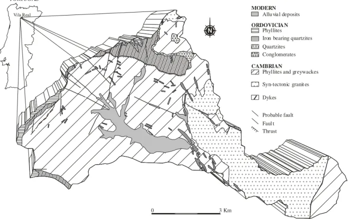
Figure 1 – Geological map of the Sordo river hydrographic basin. Adapted from Pereira (1989).

Figure 2  Soil map of the Sordo river hydrographic basin. Adapted from Agroconsultores and Coba (1991). M and P are Hayford-Gauss coordinates.

Figure 3  Location of the mapped and monitored springs. Mapped springs are represented by the bullets, springs monitored in the metasediments by the diamonds, and springs monitored in the granites by the circles. Relation between ‘fracture’ densities (shaded areas) and spring occurrence (scatter bullets). M and P are Hayford-Gauss coordinates.

Figure 4 –Procedure used to estimate the recharge associated with spring Nr 13 (see also Equation 1). Bullets represent measured discharge rates and solid lines the base flow trends. Symbols: Qf – base flow at the end of an earlier recession; Qi – base flow at the beginning of the

next recession; t1 – time corresponding to one log cycle of discharge.

Figure 5 – Location of the area used for estimation of K and n. Bullets represent the monitored dug wells, circles the four analyzed springs located inside the rectangle. Labels of bullets agree with the numbers in row “Nr” of Table 3. Shaded areas represent different ‘fracture’ densities.

Figure 6 – Median values and inter-quartile ranges for hydraulic conductivity (K), effective porosity (n) in the area of the monitored dug wells (Figure 5). Median values for the water table

depth (s) in the same area. For K and n, the median values are represented by the dots and circles, and the inter-quartile ranges by the dashed and solid thin vertical bars.

Figure 7a – Distribution of plagioclase weathering log rates (dotted histogram) and of corresponding commonly reported field log rates (white histogram; source: White and Brantley, 2003). Rate data are expressed in mol/m2.s. Prior to projection, present study log rates (cf. Table 6) were normalized by the BET surface area, i.e. were reduced by log(8.04103

).

Figure 7b – Distribution of plagioclase weathering log rates (dotted histogram) and of corresponding commonly reported laboratory log rates (white histogram; source: White and Brantley, 2003). Rate data are expressed in mol/m2.s.

Figure 8a – Distribution of biotite weathering log rates of (dotted histogram) and of corresponding commonly reported field log rates (white histogram; source: White and Brantley, 2003). Rate data are expressed in mol/m2.s. Prior to projection, present study log rates (cf. Table 6) were normalized by the BET surface area, i.e. were reduced by log(3.37104).

Figure 8b – Distribution of biotite weathering log rates (dotted histogram) and of corresponding commonly reported laboratory log rates (white histogram; source: White and Brantley, 2003). Rate data are expressed in mol/m2.s.

TABLE 1

Mineral Structural Formula Rock Type

Granites Metasediments

Quartz SiO2 36.5 25.9

K-feldspar KAlSi3O8 16.4

Plagioclase _{Na1xCaxAl1+xSi3xO8} 24.5 10.5

Chlorite (Al2.8Fe5.6Mg3.6)(Si5.3Al2.7)O20(OH)16 19.5

Biotite (Na0.3K1.7)(Mg1.5Fe2.5)(Al0.9Ti0.4Fe0.7)(Si5.2Al2.8)O20(OH)4 3.8 Muscovite (Na0.3K1.7)(Al3.6Fe0.2Mg0.2)(Si6.3Al1.7)O20(OH)4 44.1

TABLE 2

Nr M (m) P (m)

t (days) and associated year and month

R (m3₎

0 62 90 126 157 202 219 246 281 309 338 372 401 435 466

2002 2003

Jul Sep Oct Nov Dec Jan Feb Mar Apr May Jun Jul Aug Sep Oct

Q (l/s) 1 220262 481928 0.430 0.050 0.019 2.110 3.990 8.370 1.640 2.450 2.140 1.740 0.490 0.160 0.140 0.030 0.033 19471 5 220510 482983 0.400 0.040 0.050 2.440 3.500 6.490 1.290 2.680 1.440 1.470 0.430 0.160 0.080 0.032 0.078 17937 13 223457 483453 0.050 0.008 0.005 0.050 0.160 0.230 0.080 0.150 0.130 0.120 0.030 0.010 0.010 0.005 0.005 1011 14 223353 482952 0.720 0.060 0.045 2.000 2.600 2.650 2.010 2.480 2.800 2.050 0.840 0.310 0.150 0.074 0.063 15041 16 220743 479809 0.690 0.190 0.360 0.640 0.600 0.590 0.310 0.380 0.560 0.500 0.410 0.280 0.130 0.140 0.111 5741 18 220019 478505 0.350 0.220 1.630 2.180 2.050 2.720 1.910 1.840 1.750 1.440 0.570 0.350 0.150 0.086 13199 30 221199 479503 0.060 0.310 1.800 1.930 3.210 2.110 3.000 1.730 1.480 0.470 0.240 0.060 0.036 0.306 11240 34 222534 479263 0.150 0.130 0.150 0.160 0.240 0.480 0.170 0.180 0.220 0.160 0.140 0.130 0.130 0.138 0.156 3461 34A 222381 479164 0.050 0.096 0.210 0.160 0.270 0.260 0.270 0.260 0.260 0.110 0.050 0.010 0.040 0.116 831 43 222449 481779 0.032 0.035 0.060 0.140 0.120 0.130 0.140 0.130 0.070 0.040 0.050 0.040 0.041 1741 56 222147 479784 0.040 0.050 0.480 0.440 0.440 0.450 0.390 0.430 0.440 0.300 0.080 0.020 0.008 0.054 2942 57 223415 481024 0.340 0.260 0.550 4.500 18.000 3.380 0.700 0.380 0.670 0.400 0.320 0.215 15098 65 224076 479343 0.500 0.920 1.450 1.690 1.980 1.830 1.350 0.980 0.740 0.470 0.430 0.116 9477 93 225627 479589 0.170 0.090 0.092 0.050 1.000 0.860 0.390 0.210 0.150 0.112 0.104 4889 104 226659 478793 0.280 0.300 0.370 0.570 2.790 4.290 4.500 2.610 2.730 3.170 1.880 1.130 0.750 0.680 0.716 41002 110 226935 477946 0.170 0.110 0.130 0.190 3.060 4.910 5.240 2.930 1.520 0.930 0.340 30112 113 224994 480932 10.000 2.530 3.100 3.270 4.290 5.020 4.290 4.170 4.110 4.370 3.600 2.880 2.200 2.090 2.230 53551 120 226685 479675 0.440 0.080 0.160 0.530 1.010 1.030 0.940 0.980 1.000 0.940 0.440 0.410 0.330 0.116 0.092 8957 125 228488 478211 0.070 0.046 0.140 0.170 0.350 0.390 0.230 0.220 0.230 0.180 0.150 0.130 0.070 0.039 0.047 3155 140 227308 478536 0.060 0.027 0.030 0.140 0.280 0.260 0.210 0.230 0.220 0.200 0.150 0.090 0.060 0.037 0.034 3033 141 227589 477555 0.120 0.060 0.080 0.270 0.280 0.250 0.950 0.120 0.090 0.500 0.250 0.210 0.120 0.072 2524 150 228702 477164 0.055 0.170 0.640 0.760 0.280 0.280 0.340 0.190 0.090 0.090 0.089 0.092 4882 154 229302 477330 0.040 0.034 0.035 0.050 0.300 0.310 0.230 0.230 0.250 0.160 0.110 0.060 0.040 0.047 0.460 2625 156 229662 477511 0.050 0.046 0.069 0.070 0.410 0.500 0.480 0.570 0.340 0.290 0.130 0.100 0.060 0.053 0.077 3344 162 229579 476706 0.013 0.009 0.015 0.050 0.080 0.050 0.040 0.010 0.020 0.030 0.020 0.010 0.010 0.005 0.008 237 166 229791 476740 0.013 0.010 0.010 0.040 0.050 0.060 0.040 0.040 0.060 0.040 0.030 0.030 0.010 0.007 0.008 465 178 231450 478463 0.320 0.300 0.310 0.350 1.250 1.340 2.050 5.460 1.380 1.150 0.860 0.660 0.530 0.460 0.535 52195 184 230914 478269 0.140 0.150 0.160 0.140 0.160 0.990 0.650 0.780 0.690 0.730 0.500 0.150 0.070 0.059 0.060 4711 189 230156 476948 0.080 0.069 0.076 0.080 0.090 0.180 0.150 0.080 0.130 0.140 0.110 0.100 0.070 0.082 0.079 1405 195 230925 476882 0.080 0.062 0.050 0.940 1.230 0.290 0.550 0.350 0.240 0.120 0.050 0.050 0.022 4545 196 231275 477051 0.030 0.019 0.030 0.060 0.340 0.350 0.190 0.360 0.130 0.100 0.100 0.050 0.030 0.023 0.053 2753

TABLE 3 Nr 19 32 35 49 51 53 59 62 63 99 Hayford-Gauss coordinates M (m) 222164 222733 222417 223291 223187 222915 223502 223456 223788 224167 P (m) 479293 479255 479689 479650 479623 479743 479378 479252 479326 479354 Ec (S/cm) Feb 48.7 216.0 47.3 58.2 53.6 57.0 61.6 178.9 203.0 100.7 Mar 60.2 214.0 41.6 56.0 56.8 56.4 62.0 207.0 202.0 95.8 Apr 51.4 213.0 40.4 53.5 49.8 51.3 66.0 170.9 226.0 96.6 May 45.7 192.3 40.5 51.4 51.6 51.4 72.8 180.0 228.0 103.0 Jun 56.1 194.0 42.0 52.2 48.5 48.8 78.3 136.0 237.0 106.9 Jul 58.4 223.0 43.2 51.1 49.7 59.4 71.7 123.8 205.0 108.3 Aug 69.0 270.0 48.8 56.6 59.0 97.7 76.3 159.0 184.5 116.5 Sep 58.4 255.0 45.0 50.2 76.2 146.0 63.6 162.5 139.1 96.3 Oct 65.6 302.0 52.0 54.7 58.4 136.5 67.3 165.0 135.6 104.2 Nov 73.4 279.0 57.7 59.5 56.2 66.3 73.0 153.0 182.9 112.0 h (m) Feb 747.5 741.9 717.2 689.0 699.6 699.4 698.0 701.9 697.0 693.0 Mar 747.5 744.1 717.4 688.9 699.7 700.4 698.0 703.1 697.0 693.0 Apr 747.3 743.2 717.6 688.8 699.5 699.8 698.0 702.4 697.0 693.0 May 747.2 742.2 716.9 688.7 699.4 699.7 698.0 702.0 697.0 692.7 Jun 746.4 741.8 716.1 688.2 698.8 698.4 697.6 700.7 696.2 692.4 Jul 746.2 741.5 715.7 688.0 698.5 697.3 697.4 700.2 695.9 692.5 Aug 746.0 741.0 715.3 687.5 698.1 697.0 697.2 699.7 695.7 692.2 Sep 745.7 741.2 715.3 687.5 697.9 697.0 697.0 699.5 695.4 692.3 Oct 746.8 742.0 716.1 687.9 698.3 697.0 697.4 699.4 695.9 692.5 Nov 747.5 744.3 718.0 688.9 699.6 700.7 698.0 703.0 697.0 693.0

TABLE 4

Nr T Ec pH

Major inorganic compounds and concentration units

Err log(PCO2) pHin Na+ _K+ _Mg2+ _Ca2+ _HCO 3- Cl- SO42- NO3- H4SiO40 (ºC) (S/cm) mg/l mg/l mg/l mg/l mg HCO3/l mg/l mg SO4/l mg NO3/l mg H4SiO4/l % Granites 93 13.5 22.9 4.9 3.58 0.26 0.23 0.46 5.00 3.81 0.51 1.37 12.38 4.5 _-1.1 4.47 104 12.1 42.0 4.9 4.13 1.08 1.36 2.16 10.00 4.86 1.70 4.30 14.06 2.8 _-0.9 4.35 110 13.7 38.7 5.8 4.30 0.76 1.58 1.82 7.50 4.68 0.44 3.68 17.14 14.2 _-1.9 4.86 113 11.7 23.1 5.0 2.94 0.29 0.50 0.95 5.00 3.25 1.14 1.55 9.17 0.5 _-1.3 4.56 120 13.9 49.4 5.8 6.36 1.19 0.96 2.23 10.00 7.87 2.16 3.23 13.24 1.7 _-1.8 4.80 125 16.6 296.0 5.2 41.20 4.23 3.60 10.20 5.00 86.70 3.00 7.18 23.09 0.0 -1.5 4.66 140 13.3 33.3 4.9 5.75 0.20 0.33 0.67 5.00 7.60 0.65 1.64 13.44 3.3 -1.2 4.51 141 15.5 44.5 6.1 4.48 1.22 1.16 2.03 5.00 6.11 2.13 7.93 14.44 0.5 _-2.4 5.10 150 14.0 316.0 5.0 26.70 9.80 5.69 22.60 10.00 40.47 22.52 76.58 42.07 0.0 _-1.0 4.38 154 15.5 62.0 5.7 10.70 0.55 0.70 3.46 25.00 6.67 1.46 0.00 28.32 6.4 _-1.3 4.56 156 14.1 58.5 6.3 10.80 0.42 0.57 3.42 22.50 6.26 0.88 0.27 46.86 10.6 _-2.0 4.88 162 17.1 103.4 5.9 14.20 0.88 1.52 7.18 15.00 9.72 15.60 7.75 50.97 10.6 _-1.7 4.73 166 23.0 92.7 5.8 11.60 0.65 1.60 5.37 5.00 10.33 18.35 5.45 38.65 7.8 _-2.1 4.94 184 16.7 67.9 6.7 12.60 0.71 0.80 1.41 20.00 7.44 2.43 0.13 55.07 9.4 -2.3 5.07 189 18.0 111.3 6.2 19.80 0.86 1.35 4.15 17.50 15.30 7.38 16.79 48.57 2.9 -2.0 4.88 Metasediments 1 12.6 29.8 5.2 3.26 0.29 0.71 1.81 7.50 3.12 0.33 1.68 15.70 10.0 _-1.3 4.55 5 11.6 33.0 5.2 3.72 0.35 0.74 1.34 7.50 3.86 1.07 2.48 13.82 0.8 _-1.3 4.56 13 12.8 19.0 4.6 1.91 0.30 0.59 0.12 5.00 3.31 0.24 0.35 6.53 12.7 _-0.9 4.35 14 12.8 25.4 4.5 2.66 0.58 0.54 0.39 5.00 4.17 0.57 1.99 7.97 11.9 _-0.8 4.31 16 12.2 27.4 5.2 2.98 0.20 0.49 1.40 5.00 3.87 0.77 1.99 8.59 1.3 _-1.5 4.63 18 9.5 21.5 5.8 2.72 0.18 0.48 1.15 5.00 3.11 0.64 0.58 8.35 7.1 -2.1 4.94 30 11.5 41.6 5.4 5.79 0.16 0.75 1.61 5.00 9.13 1.03 0.93 10.19 3.1 -1.7 4.75 34 12.6 123.4 4.9 12.50 7.04 1.54 5.09 5.00 18.26 5.13 24.01 11.29 0.7 _-1.2 4.50 34A 13.4 143.1 4.9 17.40 2.20 2.87 6.57 7.50 32.84 3.15 12.58 12.45 2.4 _-1.0 4.41 43 14.6 41.8 5.1 3.73 0.42 1.39 2.55 7.50 4.15 0.83 5.89 12.76 8.5 _-1.2 4.50 56 11.5 41.6 5.4 3.25 0.13 0.53 1.10 5.00 3.97 0.40 1.33 10.50 4.4 _-1.7 4.75 57 11.9 29.2 5.9 3.54 0.40 0.73 1.31 7.50 3.16 0.47 2.52 14.67 5.1 _-2.0 4.91 65 12.9 104.7 5.0 7.66 0.92 4.05 7.14 10.00 5.55 24.46 8.46 14.47 8.1 _-1.0 4.41 178 17.2 175.7 6.3 20.80 2.65 6.34 8.77 30.00 14.63 28.56 14.93 49.94 7.7 -1.8 4.79 195 14.2 235.0 6.3 22.70 1.98 9.39 14.40 20.00 25.74 32.05 33.57 41.05 7.7 -2.0 4.91 196 16.2 181.6 6.3 21.40 1.88 6.89 8.33 15.00 21.53 18.62 29.32 43.79 8.6 -2.1 4.93

TABLE 5

Mineral Reaction (round-off coefficients)

Pl 4 4 -3 2 2 2 H SiO 1 1 4 2HCO Ca 1 2 Na 1 1 2 Kl 2CO O H Pl 1 2                                  x x x x x x n x Bt

0.54Bt + nH2O + 2.7CO2 + 1.51O2  Kl + 0.86Fe2O3 + 0.22TiO2 + 0.16Na+ + 0.92K+

+ 0.81Mg2+ + 2.7HCO3 + 0.81H4SiO4

Ch

0.36Ch + nH2O + 2.62CO2 + 1.5O2 + 0.07H4SiO4  Kl + Fe2O3 + 1.31Mg2+ +

TABLE 6

Nr x [Pl] (mol/l) [Bt] (mol/l) [Ch] (mol/l) Qmed (l/s) A 108 (m2) Log WPl Log WBt Log WCh

Granites 93 0.0 61.6 4.1 0.15 5.9 -13.2 -13.6 104 0.2 76.8 15.4 1.13 49.3 -13.1 -13.0 110 0.1 90.7 9.8 0.93 36.2 -13.0 -13.2 113 0.2 52.7 4.3 3.60 64.4 -12.9 -13.2 120 0.2 70.9 16.5 0.44 10.8 -12.9 -12.8 125 0.0 80 0.5 0.15 3.8 -12.9 -14.3 140 0.1 72.5 1.2 0.14 3.7 -12.9 -13.9 141 0.0 73.7 1.7 0.17 3.0 -12.8 -13.6 150 0.0 162 0.4 0.18 5.9 -12.7 -14.5 154 0.11 3.2 156 0.10 4.0 162 0.0 261.7 4.5 0.02 0.3 -12.2 -13.2 166 0.03 0.6 184 0.1 294.5 9.4 0.16 5.7 -12.5 -13.2 189 0.0 244.3 11.4 0.08 1.7 -12.3 -12.8 Metassediments 1 0.0 82.7 7.4 0.49 23.4 _-12.8 -14.1 5 0.0 72.4 7.2 0.43 21.6 _-12.9 -14.1 13 0.0 34.6 6.6 0.05 1.2 _-12.9 -13.9 14 0.0 42.2 5.5 0.84 18.1 _-12.7 -13.9 16 0.0 45.3 5.3 0.38 6.9 _-12.6 -13.8 18 0.1 48.9 4.8 1.54 15.9 _-12.3 -13.6 30 0.0 53.6 4.7 0.98 13.5 _-12.4 -13.8 34 0.0 59.3 3.6 0.16 4.2 _-12.7 -14.2 34A 0.0 65.7 10.1 0.14 1.0 _-12.1 -13.1 43 0.0 67.6 9.9 0.06 2.1 _-12.7 -13.8 56 0.1 57.7 3.7 0.35 3.5 _-12.3 -13.7 57 0.0 76.9 7.3 0.48 18.2 _-12.7 -14.0 65 0.0 77 14.8 0.95 11.4 _-12.2 -13.2 178 0.0 263.8 38.4 0.66 62.8 _-12.6 -13.7 195 0.0 216.3 24.8 0.12 5.5 _-12.3 -13.6 196 0.0 229 11 0.06 3.3 _-12.4 -14.0

FIGURE 1 + + + + + + + + + + + + + + + + + + + + + + + + + + + + + + + + + + + + + + + + + + + + + + + + + + + + + + + + + + + + + + + + + + + + + + + + + + + + + + + + + + + + + + + + + + + + + + + + + + + + + + + + + + + + + + + + + + + + + + + + + + + + + + + + + + + + + + + + + + + + + + + + + + + + + + + + + + + + + + + + + + + + + + + + + + + + + + + + + + + + + + + + + + + + + + + + + + + + + + + + + + + + + + + + + + + + + + + + + + + + + + + + + + + + + + + + + + + + + + + + + + + + + + + + + + + + + + + + + + + + + + + + + + + + + + + + + + + + + + + + + + + + + + + + + + + + + + + + + + + + + + + + + + + + + + + + + + + + + + + + + + + + + + + + + + + + + + + + + + + + + + + + + + + + + + + + + + + + + + + + + + + + + + + + + + + + + + + + + + + + + + + + + + + + + + + + + + + + + + + + + + + + + + + + + + + + + + + + + + + + + + + + + + + + + + + + + + + + + + + + + + + + + + + + + + + + + + + + + + + + + + + + + + + + + + + + + + + + + + + + + + + + + + + + + + + + + + + + + + + + + + + + + + + + + + + + + + + + + + + + + + + + + + + + + + + + + + + + + + + + + + + + + + + + + + + + + + + + + + + + + + + + + + + + + + + + + + + + + + + + + + + + + + + + + + + + + + + + + + + + + + + + + + + + + + + + + + + + + + + + + + + + + + + + + + + + + + + + + + + + + + + + + + + + + + + + + + + + + + + + + + + + + + + + + + + + + + + + + + + + + + + + + + + + + + + + + + + + + + + + + + + + + + + + + + + + + + + + + + + + + + + + + + + + + + + + + + + + + + + + + + + + + + + + + + + + + + + + + + + + + + + + + + + + + + + + + + + + + + + + + + + + + + + + + + + + + + + + + + + + + + + + + + + + + + + + + + + + + + + + + + + + + + + + + + + + + + + + + + + + + + + + + + + + + + + + + + + + + + + + + + + + + + + + + + + + + + + + + + + + + + + + + + + + + + + + + + + + + + + + + + + + + + + + + + + + + + + + + + + + + + + + + + + + + + + + + + + + + + + + + + + + + + + + + + + + + + + + + + + + + + + + + + + + + + + + + + + + + + + + + + + + + + + + + + + + + + + + + + + + + + + + + + + + + + + + + + + + + + + + + + + + + + + + + + + + + + + + + + + + + + + + + + + + + + + + + + + + + + + + + + + + + + + + + + + + + + + + + + + + + + + + + + + + + + + + + + + + + + + + + + + + + + + + + + + + + + + + + + + + + + + + + + + + + + + + + + + + + + + + + + + + + + + + + + + + + + + + + + + + + + + + + + + + + + + + + + + + + + + + + + + + + + + + + + + + + + + + + + + + + + + + + + + + + + + + + + + + + + + + + + + + + + + + + + + + + + + + + + + + + + + + + + + + + + + + + + + + + + + + + + + + + + + + + + + + + + + + + + + + + + + + + + + + + + + + + + + + + + + + + + + + + + + + + + + + + + + + + + + + + + + + + + + + + + + + + + + + + + + + + + + + + + + + + + + + + + + + + + + + + + + + + + + + + + + + + + + + + + + + + + + + + + + + + + + + + + + + + + + + + + + + + + + + + + + + + + + + + + + + + + + + + + + + + + + + + + + + + + + + + + + + + + + + + + + + + + + + + + + + + + + + + + + + + + + + + + + + + + + + + + + + + + + + + + + + + + + + + + + + + + + + + + + + + + + + + + + + + + + + + + + + + + + + + + + + + + + + + + + + + + + + + + + + + + + + + + + + + + + + + + + + + + + + + + + + + + + + + + + + + + + + + + + + + + + + + + + + + + + + + + + + + + + + + + + + + + + + + + + + + + + + + + + + + + + + + + + + + + + + + + + + + + + + + + + + + + + + + + + + + + + + + + + + + + + + + + + + + + + + + + + + + + + + + + + + + + + + + + + + + + + + + + + + + + + + + + + + + + + + + + + + + + + + + + + + + + + + + + + + + + + + + + + + + + + + + + + + + + + + + + + + + + + + + + + + + + + + + + + + + + + + + + + + + + + + + + + + + + + + + + + + + + + + + + + + + + + + + + + + + + + + + + + + + + + + + + + + + + + + + + + + + + + + + + + + + + + + + + + + + + + + + + + + + + + + + + + + + + + + + + + + + + + + + + + + + + + + + + + + + + + + + + + + + + + + + + + + + + + + + + + + + + + + + + + + + + + + + + + + + + + + + + + + + + + + + + + + + + + + + + + + + + + + + + + + + + + + + + + + + + + + + + + + + + + + + + + + + + + + + + + + + + + + + + + + + + + + + + + + + + + + + + + + + + + + + + + + + + + + + + + + + + + + + + + + + + + + + + + + + + + + + + + + + + + + + + + + + + + + + + + + + + + + + + + + + + + + + + + + + + + + + + + + + + + + + + + + + + + + + + + + + + + + + + + + + + + + + + + + + + + + + + + + + + + + + + + + + + + + + + + + + + + + + + + + + + + + + + + + + + + + + + + + + + + + + + + + + + + + + + + + + + + + + + + + + + + + Vila Real 0 3 Km N + + + + + + + + + + + + + + + + + + + + + + + + + + + + + + + + + + + + + + + + + + + + + + + + + + + + + + + + + + + + + + + + + + + + + + + + + + + + + + + + + + + + + + + +

Allu vial deposits

MODERN

ORDOVICIAN

CAMBRIAN

Phyllites

Iron bearing quartzites Quartzites

Conglomerates Phyllites and greywackes Syn-tectonic granit es Dykes Probable fault Faul t Thrust PORTUGAL

FIGURE 3 218000 220000 222000 224000 226000 228000 230000 232000 M (m) 478000 480000 482000 484000 P ( m )

kilometers of 'fracture' per square kilometer of area

0 10 20

Mapped spring

1 to 2 2 to 3

Monitored spring (metassediments) Monitored spring (granites)

FIGURE 4 0.001 0.010 0.100 1.000 0 50 100 150 200 250 300 350 400 450 500 Time - t (days) Discharge rate - Q (l/s ) Q_f Q_i t1

FIGURE 5 222500 223000 223500 224000 M (m) 479250 479500 479750 P ( m ) 19 32 35 49 51 53 59 62 63 99 34 34A 56 65

kilometers of fracture per square kilometer of area Sordo river hydrographic basin

FIGURE 6 0 2 4 6 8 10 12

Mar Apr Mai Jun Jul Aug Sep Oct Nov

Month n (%), K ( 10 -6 m /s) 0.0 0.5 1.0 1.5 2.0 2.5 3.0 3.5 s (m ) K n s

FIGURE 7a -17 -16.5 -16 -15.5 -15 -14.5 -14 -13.5 -13 -12.5 -12 Log W_Pl 0 4 8 12 16 20 24 28 N u m b e r o f o b se rv a ti o n s 0 1 2 3 4 5 6 7 N u m b e r o f o b se rv a ti o n s

Present study log rates normalized by BET surface area (left axis) Commonly reported field log rates (right axis)

FIGURE 7b -15 -14.5 -14 -13.5 -13 -12.5 -12 -11.5 -11 -10.5 -10 Log W_Pl 0 2 4 6 8 10 12 14 16 18 20 N um be r of obs erva ti ons 0 1 2 3 4 5 6 N um be r of obs erva ti ons

Present study log rates normalized by fracture surface area (left axis) Commonly reported laboratory log rates (right axis)

FIGURE 8a -18 -17.5 -17 -16.5 -16 -15.5 -15 -14.5 -14 -13.5 Log W_Bt 0 1 2 3 4 5 6 7 8 9 N um be r of obs erva ti ons 0 1 2 3 N um be r of obs erva ti ons

Present study log rates normalized by BET surface area (left axis) Commonly reported field log rates (right axis)

FIGURE 8b -18.5 -18 -17.5 -17 -16.5 -16 -15.5 -15 -14.5 -14 -13.5 Log W_Bt 0 1 2 3 4 5 6 7 8 9 N um be r of obs erva ti ons 0 1 2 3 N um be r of obs erva ti ons

Present study log rates normalized by BET surface area (left axis) Commonly reported field log rates (right axis)