I
T
RABALHO
F
INAL DE
M
ESTRADO
DISSERTAÇÃO
HOW WELL CAN SIMPLE RULES TRACK THE BEHAVIOR OF
THE ECB?
POR
II
MESTRADO EM
ECONOMIA MONETÁRIA E FINANCEIRA
TRABALHO FINAL DE MESTRADO
DISSERTAÇÃO
HOW WELL CAN TAYLOR RULES TRACK THE BEHAVIOR OF
THE ECB?
ALUNO:
Jodzinda Irvina De Almeida Pires
ORIENTAÇÃO:
Professora Doutora Maria Cândida Rodrigues Ferreira
JÚRI:
Presidente: Professor Doutor António Manuel Pedro Afonso
Arguente: Professor Doutor Emanuel Cláudio Reis Carvalho Leão
III
HOW WELL CAN TAYLOR RULES TRACK THE BEHAVIOR OF THE ECB?
Abstract
Taylor (1993) proposed a simple rule that drew attention of economists, scholars and central bankers due to its simplicity and outstanding description of Fed’s behavior in 1980s. Over time, different versions of Taylor Rules (TRs) emerged aiming to evaluate the conduct of monetary policy of US and other countries, including recently the Euro area. Attending to the fact that previous studies concerning the Euro area are limited by short-time span of data, in this dissertation we analyze the performance of TRs in tracking the behavior of the European Central Bank (ECB), through a simple forward-looking approach and relatively long span of data (which comprises the two more severe economic turmoil of XXI century so far). The results obtained confirm that TRs, in general, track the ECB behavior very closely, mainly due to the gradualism of the ECB monetary policy. However, during economic turbulence we verified some deviations from the rule. The small magnitude of our empirical results reminds us that TRs are rough simplification of a complex reality.
JEL Classification: E52,E58
IV
QUAL A CAPACIDADE DAS REGRAS DE TAYLOR DE DESCREVER O
COMPORTAMENTO DO BCE?
Resumo
Devido à sua simplicidade e excelente descrição da política monetária dos EUA entre os anos de 1987 e 1992, a Regra de Taylor (RT) (1993) atraiu a atenção dos académicos, analistas e decisores de política monetária; e, ao longo do tempo, foram surgindo diferentes versões de regras de Taylor, sendo cada versão uma tentativa de as tornar num instrumento mais prático a ser usado na avaliação da política monetária dos EUA e de outros países, incluindo recentemente a área do Euro. Atendendo ao facto de que os estudos anteriores associados à área do Euro estão, de certa forma, limitados por poucos dados disponíveis, nesta dissertação, analisamos as RT tendo em conta uma base de dados relativamente mais abrangente (que engloba, até então, as duas turbulências económicas mais severas do século XXI). Através de uma abordagem
forward-looking, o objetivo é de verificar a capacidade das simples regras de Taylor em descrever as
decisões de política monetária do Banco Central Europeu (BCE). Os resultados obtidos confirmam que as RT, no geral, fazem uma boa descrição da política monetária do BCE, principalmente devido ao ajuste gradual da política monetária. No entanto, face às turbulências económicas verificam-se desvios das RT. Além disso, a magnitude dos resultados estatísticos remete-nos para o facto de que as RT são uma simplificação de uma realidade muito complexa.
Classificação JEL: E52, E58
V
Index
I. INTRODUCTION ... 1
II. THEORETICAL AND EMPIRICAL BACKGROUND ... 4
2.1BACKGROUND ON TAYLOR RULES ... 4
2.2OVERVIEW OF EMPIRICAL RESULTS FROM SELECTED LITERATURES ... 9
III. EMPIRICAL MODEL ... 12
3.1MODEL SPECIFICATION ... 12
3.2DATA AND VARIABLES ... 13
3.3DATA DIAGNOSIS ... 15
3.4ESTIMATOR ... 17
IV. EMPIRICAL RESULTS ... 18
4.1BASELINE SPECIFICATION RESULTS ... 19
4.2CROSS-CHECKING DIFFERENT SAMPLE PERIOD ... 23
4.3CHANGE IN THE ECONOMIC STRUCTURE ... 24
4.4IMPACT OF ADDITIONAL EXPLANATORY VARIABLES ... 27
V. CONCLUSION ... 29
VI. REFERENCES ... 31
VII. ANNEX... 34
Annex A ... 34
Annex A1: Description Of The Variables And Respective Sources. ... 34
Annex A2: Summary Statistics ... 38
Annex A3: Tests For Stationarity ... 38
Annex A4: Endogeneity Test ... 39
Annex A5: Tests For Heteroskedasticity ... 39
Annex A6: Serial Correlation Test ... 40
Annex A7: Cross-Checked Results; Estimantes Of TR In The Euro Area -1994:01-2011:12 – Other Estimators. 41 Annex A8: Cross-Checked Results; Estimantes Of TR In The Euro Area -1999:01-2011:12 – Different Sample. 42 Annex A9: Cross-Checked Results; Estimantes Of TR In The Euro Area- 1994:01-2011:12–Exclud Expected Realized Output Gap as Regressor. ... 42
1
I.
Introduction
Most economic scholars consider that in the short-run, optimal monetary policy response to economic shocks should combine some sort of interest rate rules involving a certain level of discretion and set of inflation targets.
Proponents of simple interest rate rules argue that implementing monetary policy by means of rules provide low probability of time inconsistence problem and, consequently, of low inflation bias. Although simple rules cannot account completely for unexpected circumstances,
they satisfy the need for transparency, adequate communication and robustness (e.g., Peersman
and Smets, 1999; Orphanides, 2007). Furthermore, many foresight or rational expectation models require the presence of systematic (rule-like) behavior on the part of the central banks for the equilibrium rate to be found.
The most popular rule in the economic literature stems from Taylor (1993) in which the key interest rate set by the Federal Reserve System (Fed) is described as a linear combination of inflation and output gap. That is, a reaction function that describes how Fed should attain its two-fold mandates (i.e. control of inflation as well as the maintenance of low business cycle fluctuations).
Given the Taylor rule (TR) simplicity and its outstanding description of the behavior of the Fed funds rate during the 1987 and 1992 – a period of long expansions and short recessions – it rapidly drew attention of economists, analysts and central bankers. Over time, different versions of TR emerged in an attempt to make it a better and actualized tool for policy makers to evaluate the conduct of monetary policy of many central banks, including recently the
2
European Central Bank (ECB) (Asso et al, 2010, give detailed discussion on TR influence on the practice of central banking).
As responsible for conducting the monetary policy of the Euro area, the ECB has an overriding mandate – price stability over the medium term – that is not dual as suggested by the TRs framework. However, in line with the ECB Governing Council monetary policy strategy, built on an analytical framework which is based on two pillars - monetary and economic analysis (ECB, 2011, p.69) – one can find room for TRs in the first pillar strategy given that output gap measures are included in the set of leading indicators for future inflation. In addition, this stability-oriented monetary policy strategy causes the ECB to behave in a systematic manner; a feature that we expect TRs to be able to track.
Considering that previous studies on TRs for the Euro area were limited by short-time span of data available and also that there are few studies analyzing the impact of the recent economic turmoil in context of TRs, in this dissertation, we intend to contribute to the literature by dealing with: relatively long time span of data – a sample period that comprises the launch of the euro as single currency and two major economic turbulence (subprime crisis and the subsequent European sovereign debt crisis); three different measures of output gap, in which we specially include the OECD’s composite leading indicator (CLI), given that it aims to reveal early signs of economic turning-points and move in the same direction as the business cycle. Through a simple forward-looking approach with a smoothing parameter we aim to assess the TRs’ performance in tracking the ECB monetary policy-making. To complete this assessment, we extended the rule by a set of additional variables.
The results found do not differ much from those already seen in the literature, as will be mentioned through the dissertation: simple TRs seem to track the ECB policy decision very
3
closely (which testifies in favor of ECB’s systematic behavior). The use of Hodrick-Prescott-filtered industrial production output gap points to output gap or the overall economic performance as the main trigger of ECB’s intervention, while the use of annual growth in the industrial production index (and the CLI) as proxy for output gap point that ECB policy rate reacts not only to inflation but also to the output gap ( both results are perfectly in line with the ECB’s main objective of price stability as output gap measures serve as leading indicator of inflationary pressure ).
Another result confirmed in this dissertation is the fundamental rule of interest rate smoothing in enhancing the fit of the TR: the particularly high and robust value of the smoothed interest rate coefficient is consistent with the ECB’s cautious policy intervention and suggests that past interest rates are the main determinants of actual policy rates.
Nevertheless, the main advantage of TRs – simplicity – turns out to be their main weakness: TRs, in essence, capture the general course of a stability-oriented central bank such as the ECB, but leave out a wide range of information needed to backup a central bank’s decision. This may justify the small (inflation and output gap) coefficients responses obtained. In fact, TRs are rough simplification of a complex, but may be used as an additional informative indicator.
The rest of the paper is organized as follows: section 2 reviews the theoretical and empirical background; section 3 develops the econometric model; section 4 reports the empirical results; section 5 draws conclusions.
4
II.
Theoretical and Empirical Background
In this section we first present a brief background on TRs and then systematize the empirical results obtained from selected literature regarding the Bundesbank and the ECB.
2.1 Background on Taylor Rules
The economic literature related to Taylor-like rules is considerably vast. The different Taylor rule specifications vary from theoretical to empirical perspectives regarding: backward- and/or forward-looking perspective; measures of inflation and output gap; policy rate proxy; estimation methods; instruments and additional explanatory variables chosen; type of data; geography; sample period; models (e.g., Dynamic Stochastic General Equilibrium) and so on. Each line of research on TRs has been an attempt to make it a more actualized and operational tool.
Clearly a thorough survey on TRs literature is beyond the scope of this dissertation; hence, we modestly review the ones that contributed the most to the present analysis.
We start by Taylor (1993) which proposed a simple rule that states that Fed should set its short-term nominal interest rate (it) – federal funds rate – in response to the equilibrium real rate
( r ); inflation gap (πt - π ) defined as the deviation of inflation (πt) from its target ( π ); and
output gap (xt = Yt - Yt*) defined as the deviation of real GDP (Yt) from its potential level (Yt*).
The rule is depicted as follows:
5
Implicitly, the rule recommends central banks to match their policy rate to the nominal interest rate ( r + πt) as inflation rate and output are at their respective long-run levels.
Taylor gave same emphasis to both inflation and output stabilization, by assuming that
the betas of inflation (βπ) and output gap (βx) were equal to 0.5, which implies that Fed should
raise the fed funds rate about 0.5 percent as inflation (or output) raises 1 percent above the target.
Additionally, he assumed that the equilibrium real interest rate ( r ) and inflation target ( π )
are equal to 2 percent.
With these values attributed in Taylor (1993), the TR entails what is called “Taylor principle”, which assumes that βπ should be greater than a unit, implying that as inflation
deviates from its target, nominal interest rates (it) should raise more than one-for-one
(sufficiently) to cause an increase in the real rates ( r ); where a βπ <1 would imply deficient policy response to rising inflation, tending to aggravate inflationary pressure. This principle also assumes that βx should be positive but not necessarily above a unit, meaning that in order to
achieve a stabilizing impact on output, monetary policy should accommodate shocks from the supply side. Such principle is consistent with the properties of model-specific optimal and more complex policy rules and provides a mean to anchor inflation over time. Such principle becomes visible when Taylor reaction function is rearranged as follows:
(2) it* = 1.5 πt + 0.5xt + 1 where xt =(Yt - Yt*)
Clarida et al (1998) proposed a forward-looking version of TRs in which it is claimed that by considering inflation and output forecasts it is possible to incorporate a broad array of
6
information taken into account in monetary policy decision-making. This version of TRs comes as
(3) it* = r + βπ (﹝Etπt+n |Ω﹞ - π ) + βx(Ext |Ω)+ εt
where x denotes the measure of average output gap ((EYt |Ω) - Yt*); E denotes the
expectation term; πt+n stands for inflation rate at t+n; π is a constanttarget inflationrate; (Ωt) is the set of information available to policy makers at the time of decision-making regarding the short-run interest rate, and εt denotes the error term (assumed to be i.i.d).
Given the environment of pervasive uncertainty faced by policy makers, it has been
argued that they rather follow the “Brainard conservatism”(see Brainard, 1967) and implement
monetary policy in a rather cautious and sluggish fashion. Hence, partial interest rate adjustment is modeled as
(4) it = (1 – ρ)it*+ ρit-1 + υt
Where it* stands for target nominal interest rate; ρ ∈ (0, 1) denotes the degree of
smoothing of the interest rates; and υt denotes an exogenous random walk shock to the interest
rate.
Adding this partial adjustments into the equation (3)1 and assuming that there are no systematic forecast errors we can re-write the reaction function in terms of realized variable as follows
(5) it = ( 1 – ρ) α + ( 1 – ρ) βπ(πt+n - π ) + ( 1 – ρ)βx xt+n + ρit-1 + εt ;
1 At this step we get the following eq.: i
t = (1 – ρ) ( r + βπ (﹝Etπt+n |Ωt﹞ - π )) + βx (〔EYt |Ωt 〕- Yt*)) + ρit-1 +
7
where rt* stands for target interest rate; α = ( r - βπ π ); xt+n stands for the measure of
average output gap and πt+n stands for inflation rate at time t+n; π a constant target inflation
rate; ρ ∈ (0, 1) denotes the degree of smoothing of the interest rates; and εt denotes the error
term .
Nevertheless, Rudebusch (2002) contradicts interpretation of ρ as monetary policy inertia, suggesting that ρ could be interpreted as persistent shocks faced by central banks and that the distinction between partial adjustment and serially correlated shocks is not clear. Gerlach-Kristen (2004) finds that ρ is mainly the result of omitted or unobserved variables, while Sauer and Strum (2007) advocate that it is an indication of a “too little and too late” policy rate response to changes in the economic outlook. Castelnuovo (2007) used modified models in first-differences to assess Rudebusch (2002) claims (for the case of the Euro area). His results confirm the importance of the lagged interest rate, but do not rule out the influence of the serially correlated shocks when fitting simple Taylor-like rules.
Another contribution to the TRs literature is related to the application of large number of explanatory variables as inputs in the TR aiming at the identification of relevant macroeconomic variables to monetary policy decision-making. These variables (among many others) include: unemployment rate (e.g., Clarida et al, 2000), exchange rate (e.g., Molodtsova et al, 2011), annual growth in the monetary aggregate (e.g., Ullrich, 2003; Gerdesmeier and Roffia, 2004), asset prices (e.g., Cecchetti et al, 2000), interest rate spread (e.g., Dotsey, 1998; Belke and Klose (2010); financial condition or stability index composed by indicators such as fiscal indicators, stock valuations, private sector expectations, international commodity prices, credit quality, etc,
8
that capture the vulnerability of the financial market, resilience of the banking system and external and internal vulnerability (e.g., Albulescu, 2010; Castro, 2011).
Concern regarding the stationarity of the variables is also an issue dealt with in the TRs literature. In some research papers, authors assume that relevant variables are stationary (e.g., Clarida et al. 2000), while in few other papers authors use variables in first differences (e.g., Orphanides, 2003) or implement techniques such as the error-correction, cointegration approach (e.g., Gelarch-Kristen, 2003; Ruth, 2007; Sauer and Strum, 2007) to avoid spurious results.
Other issues are associated with the use of real-time data instead of ex-post revised data. Orphanides (2001) emphasized the preeminence of using real-time data, the information available to central banks at the time they consider monetary policy decisions, in policy reaction functions. Many recent papers have been dealing with this issue; for instance, Gorter et al (2008) findings suggest that the ECB’s monetary policy is stabilizing when real time expected inflation and output are used as opposed to the use of ex-post revised data (see also Orphanides, 2004; Gerdesmeier and Roffia, 2005; Belke and Klose, 2011 among others). However, Sauer and Strum (2007) suggest that real-time industrial production index data does not add much to the TR performance for the Euro area; in addition, Marcellino and Musso (2010) pointed out that real-time estimates of the Euro area output gap are associated with reasonable high degree of uncertainty and perform poorly as leading indicator for future inflation.
Given its simplicity and despite of its limitations (e.g., inability to assure that past mistakes will not be repeated (Orphanides, 2003)), over time Taylor-like rules became considered as a valuable guideline for policy makers (because TRs may enhance transparency
9
and monetary policy communication) and for the financial markets to evaluate the conduct of monetary policy of many central banks, including recently the European central bank (ECB).
As responsible for conducting the monetary policy of the Euro area, the ECB has an overriding mandate – price stability over the medium term (ECB, 2011, p.64) – that is not dual as suggested by the TRs framework. However, in line with the ECB Governing Council monetary policy strategy, built on an analytical framework based on two pillars – monetary and
economic analysis (ECB, 2011, p.69) – one can find room for TRs, given that output gap
measures are valuable leading indicators for future inflation. In this context, a number of researchers were motivated to examine the potential usefulness of TRs as an informal policy guide for the ECB. For instance, some studies focused in estimating Taylor-like rules for the “fictitious” ECB prior to 1999 when ECB was not yet in charge of the Euro area monetary policy (e.g., Peersman and Smets, 1999; Gerlach and Schnabel, 2000); Other studies estimate and compare the ECB monetary policy with a benchmark such as the Bundesbank (e.g., Faust et al, 2001), or the Federal Reserve System (Fed) (e.g., Ullrich, 2003), just to name a few.
2.2 Overview of empirical results from selected literatures
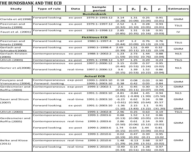
This section presents in the Table I an overview of the empirical results of different Taylor rule estimations regarding the Bundesbank and the ECB from selected literature, most of them mentioned above.
We start by presenting TRs estimates for the Bundesbank attending to the fact that due to its outstanding anti-inflationary monetary policy performance, it became a benchmark of monetary policy for European countries. Consequently, ECB was designed to follow the Bundesbank policy-making preferences (in order to inherit some credibility since there was no
10
track record proving ECB’s reputation). Therefore, most studies on ECB monetary policy compare Bundesbank (and /or Fed’s) reaction functions to the hypothetical ECB prior to 1999 and also to the actual ECB reaction functions.
A first look at the Table I shows that TRs produce a variety of results under different specifications and sample periods; some results are very similar while others seem discrepant.
For instance, the inflation coefficient response, βπ,rangesfrom 6.62 to values very close to zero
such as 0.08 or even negative ones.
TABLE I: OVERVIEW OF EMPIRICAL RESULTS OF TAYLOR RULE ESTIMATIONS REGARDING THE BUNDSBANK AND THE ECB
Study Type of rule Data Sample
period α βπ βx ρ Estimators
Forward looking ex-post 1979:3–1993:12 3.14 1.31 0.25 0.91 (0.28) (0.09) (0.04) (0.01) Forward looking ex-post 1979:1–1997:12 2.52 1.3 0.28 0.93
(0.32) (0.10) (0.05) (0.01) Forward looking ex-post 1985:1–1998:12 2.85 1.31 0.18 0.91
(0.85) (0.35) (0.16) (0.03) Forward looking ex-post 1980:1–1997:4 3.87 1.2 0.76 0.76
(0.44) (0.09) (0.13) (0.13) Forward looking ex-post 1990:1–1998:4 2.65 1.51 0.49 0.32
(0.39) (0.11) (0.12) (0.19)
Contemporaneous ex-post 1988:1–2002:2 1.23 2.73 1.44 0.88 NLS (1.59) (0.55) (0.76) (0.04)
Ullrich (2003) Contemporaneous ex-post 1995:1–1998:12 1.97 1.25 0.29 0.23 TSLS Contemporaneous ex-post 1997:1-2006:12 3.15 0.09 0.37 0.95
(0.40) (0.53) (0.24) (0.02) Forward looking real-time 1997:1-2006:12 3.6 1.39 1.52 0.86
(0.15) (0.53) (0.22) (0.04) Contemporaneous exp-post 1999:1-2003:10 0.18 0.08 0.03 0.90 Forward -looking 1999:1-2003:10 0.38 0.42 0.03 0.84 Contemporaneous exp-post 1999:1–2002:1 2.6 0.45 0.30 0.72 GMM (0.06) (0.11) (0.07) (0.04) Contemporaneous ex-post 1991:1-2003:10 4.81 -0.84 1.45 0.94 NLS (2.82) (-0.89) (1.99) (25.50)
Forward looking real-time 1991:1-2003:10 -6.23 6.62 9.24 0.98 GMM (-0.61) (0.90) (0.64) 35.57
Forward looking ex-post 1991:1-2003:10 -1.36 2.15 1.1 0.91
(1.10) (3.83) (3.22) (31.20) GMM Ullrich (2003) Contemporaneous 1999:1–2002:8 2.96 0.25 0.63 0.19 TSLS Contemporaneous ex-post 1999:1-2003:6 0.88 1.52 1.12 0.86 (0.13) (0.08) (0.05) (0.01) Contemporaneous real-time 1999:1-2003:6 2.86 0.61 2.14 0.99 (0.50) (0.06) (0.12) (0.01) Forward looking ex-post 1999:1-2003:6 1.74 0.64 1.44 0.81
(0.15) (0.07) (0.04) (0.01) Contemporaneous ex-post 1999:1-2010:6 0.02 0.47 0.39 0.95
(0.19) (0.35) (0.21 (0.02 Contemporaneous real-time 1999:1-2010:6 1.48 -6.13 3.68 0.97
(1.29) (6.29) (3.31) (0.02) Forward looking real-time 1999:1-2010:6 -0.49 0.14 1.28 0.97
(0.33) (0.51) (0.56) (0.02) Belke and Klose
(2011)
GMM
Actual ECB
Gerdesmeier and Roffia (2004) Sauer and Strum (2007) Gerdesmeier and Roffia (2005) Fourçans and Vranceanu (2004) GMM GMM GMM Gerlach-Kristen (2003) Gorter et al(2008) NLS Gerlach and Schnabel(2000) Faust et al. (2001) IV Fictitious ECB Peersman and Smets (1999) TSLS Bundesbank Clarida et al(1998) GMM Peersman and Smets (1999) TSLS
11
Note: standard errors in parentheses (when available); The contemporaneous TR refers to: rt = ( 1 – ρ) α +( 1 – ρ) βπ πt+( 1 – ρ)
βxxt + ρrt-1 + εt; Forward-looking TR refers to: it = ( 1 – ρ)( r + βπ (﹝Etπt+n |Ωt﹞ - π )) + βxxt+ ρit-1 + εt ,( xt = (EYt |Ωt ) -
Yt*); GMM stands for generalized method of moments; TSLS stands for Two-Stage Least Squares; NLS stands for nonlinear
least-squares; and the IV stands for instrumental variables estimator.
As for the output gap response coefficient, βx, the Table I shows that, in overall, it
complies with the Taylor principle (βx >0), which may indicate that the ECB reacts to the
economic activity to the extent it poses threats to price stability (possibility identified in the Economic analysis).
Also, it is evident that the coefficient responses regarding Bundesbank’s and the “fictitious” ECB’s monetary policy reveal small differences (probably because of the Germany’s economic importance and, consequently, large weight in the calculation of the fictitious ECB’s interest rate); both central bank’s reaction functions fulfill the Taylor principle (i.e., βπ >1, βx >0)
andreflect a consistent anti-inflationary philosophy.
Next, we observe that, in general and independently of the specifications, we have positive and high degree of interest rate smoothing (ρ). This suggests that the ECB has engaged in interest-rate smoothing in its monetary policy and that actual short-term interest rate depends heavily on its past value, or decisions taken beforehand by the ECB Governing Council (fact which attest the important role of credibility in monetary policy).
Concerning the type of data, the use of real-time data seems to improve the ECB’s policy rate response to inflation gap (βπ) relative to the use of ex-post revised data.
This brief survey also suggests that according to the Taylor principle (i.e., βπ >1, βx >0),
the actual ECB adopts a destabilizing policy regarding inflation and appears to give more emphasis to the output. However, given the ECB’s anti-inflation philosophy, this might be an indication that the ECB loosened policy to stabilized output while creating credibility to anchor
12
inflation expectations, or TRs, more specifically, the Taylor principle is not in harmony with the reality of the actual ECB.
Interestingly and regardless of the criticisms undergone by the TRs, this kind of rule continues to be analyzed by researchers and economists over the years.
III.
Empirical Model
In this section we present the econometric model, the definition of the variables, the diagnosis of the data and introduce the estimator used. The regressions are based upon aggregated data of the Euro area (EA), not regarding the asymmetric nature of shocks affecting each member state of the EMU and the heterogeneity that exist among them (since single monetary policy is not able respond to country-specific shocks). STATA is the statistical software chosen to carry out our analysis.
3.1 Model specification
We followed the type of Clarida et al (1999) reaction functions, without giving specific
emphasis to the real interest rate, and estimated a simple TR model as depicted in the equation (6):
(6) it = α + βπ (πt+p- π ) + βxxt+q + ρit-1 +εt .
where it stands for the money market interest rate; α is a constant; p and q correspond to the
time horizon for inflation and output gap expectations, respectively; πt+p - π denotes the
inflation gap – deviation of expected realized inflation(πt+p) at time t+p from its target ( π ),
13
as assumed in the original TR; xt+q represents the expected realized output gap at time t+q (p
and q denotes time horizon for inflation and output gap which happens to be different); βπ and βx
stands for the interest rate response to inflation and output gap respectively; ρ denotes the interest rate smoothing term; and εt denotes the residual term.
3.2 Data and variables
To deal with the short time span of data available for the actual ECB, we considered the beginning of the second stage of Economic and Monetary Union (EMU) and used monthly data covering the sample period 1994:01 to 2011:12. The estimations are carried out in levels and
based upon ex-post revised data. In the Annex A1 all variables are explained in more detail, and
in the Annex A2 we have the summary statistics.
As depicted in the eq. (6) the three main variables are: short-term nominal interest rate (it), inflation rate (π
)
and the output gap (xt).In normal circumstances, short-term money market rates such as the Euro Overnight
Index Average (EONIA) is very close to the main policy rate, namely the Main Refinancing Operation (MRO) – minimum bid rate. Besides, the data on ECB key interest rates is not available on monthly (or quarterly) frequency, which makes it difficult to use any of the key rates directly in the reaction function. Therefore, we deemed appropriate to use the EONIA as proxy for the policy rate, which is in line with most TRs empirical work concerning the Euro area (e.g., Gerdesmeier and Roffia, 2005).
With regard to the inflation rate, it is measured by the year-over-year growth rate in the overall Harmonized Index of Consumer Prices (HICP). The inflation target is set according to
14
the definition of the Governing Council of the ECB, that is, bellow but close two percent over the medium term.
As for the output gap, we encounter two main issues: first, there is no monthly data available for real GDP; second, potential output is not observable. Therefore, we have to find proxies for both variables.
To deal with the lack of monthly real GDP data, some scholars implement linear interpolation methods such as Chow and Lin (1971) procedure to convert quarterly real GDP series into monthly series. However, attending to the fact that the Industrial Production (IP)
index displays a strong co-movement with the GDP2, we don’t go through linear interpolation
methods, but use annual growth rate in the overall IP as proxy for the annual growth rate in the
real GDP instead.
To circumvent the potential output issue and get output gap measures, we took three different approaches, and hence started our analysis by using three different proxies for the output gap, which by definition fluctuate around zero mean:
1) The standard HP output gap: measured as the deviation of the logarithm of the annual growth of industrial production (IP) from its HP trend. Following e.g., Gerdesmeier and Roffia (2004) and Clarida et al (1998); we employed Hodrick-Prescott (HP) filter – a mathematical technique used to separate the cyclical component of in output from the growth component – with the smoothing parameter set to 14.400 for monthly series to fit a trend to the IP index data (Annex A1);
2
15
2) The IP output gap: measured by the annual growth of the index as proxy for the output
gap (e.g.,Fourçans and Vranceanu, 2004);
3) The CLI output gap: The two aforementioned output gap proxies are standard in the literature. In addition to it, we found interesting to proxy output gap by the annual growth of the OECD composite leading indicator (CLI), considering that (though it gives more qualitative than quantitative indication) it comprises a number of selected macroeconomic indicators and aims to forecast cycles or turning-points in the reference
series chosen as proxy for economic activity (in this case, the IP index) (Annex A1).
We finalize our analysis by extending our baseline specification to consider the effect of
other variables such as federal fund rate, Dow Jones Euro Stoxx 50 index, exchange rates, annual growth of monetary aggregate (M3) gap on the augmented TR. We also included an interest rate spread variable and sovereign (Greek and Portuguese) risk premium (see Annex A1), attending to the fact that there is a significant issue regarding the role risk plays in departures of policy from the rule.
3.3 Data diagnosis
At this stage we carry out the diagnosis of our time series with regard to the stationarity
and endogeneity of the variables, the heteroskedasticity and serial correlation of the error term. In addition, we check the multicollinearity effect on the model and, finally, determine the time horizon.
In order to check the stationarity, we employed the modified Dickey-Fuller test (DF-GLS), which has the best overall performance in terms of small-sample size and power
16
compared to the ordinary Dickey-Fuller test; we complemented this test by employing the Kwiatkowski-Phillips-Schmidt-Shin (KPSS). The tests resulted that the short-term money market rate, inflation, and the growth rate in the IP index are nonstationary I (1) variables. The standard HP output gap is stationary I (0) by construction. The CLI as well as its annual growth
rate are also stationary I (0). The stationarity test results are available in the annex (see Annex
A3).
In fact, we found that the error term resulting from a linear combination between the variables is a stationary I (0) process. For this reason, the variables are cointegrated and hence, any regression relationship between those variables is non-spurious. Therefore we proceeded by using the variables in terms of level as opposed to first differences.
Regarding endogeneity, contrary to what is expected, the endogeneity test defined as the
difference of two Sargan-Hansen statistics (see Annex A4), failed to reject the null hypothesis,
and hence, inflation gap as well as output gap could be treated as exogenous.
To test for heteroskedasticity, we used tests such as Breusch-Pagan/ Cook-Weisberg (see
Annex A5). Their rejection of the null hypothesis ascertains that the variance of the residuals is not constant over time. As result, the model is corrected to be robust to this fact.
The serial correlation test, Cumby-Huizinga test, failed to reject the null which states that
there is no serial correlation (see Annex A6). This calls for feasibility of least square estimates
and no need for model correction accounting for autocorrelation.
The degree collinearity of the variables was tested through variance inflation factor (VIF), which results came out no greater than 10, implying that multicolinearity does not represent a problem to the model. Besides, STATA automatically removes the variables that present collinearity problem.
17
Finally, we address the issue regarding the appropriate target horizon for both inflation (p) and output gap (q). There is no consensus about it, moreover, the ECB monetary strategy does not specify a fixed time horizon for policy stance, though it has a medium term (one to two years) target for inflation, inflation and economic activity forecasts over two to three years. The time horizon used here is not chosen randomly: after running several regressions with different horizons, the model was chosen based on link test (an option built into STATA) model specification, Root Mean Squared Errors (RMSE), the Akaike’s (AIC) and Schwarz's Bayesian (BIC) information criteria. The time horizons implemented in this exercise are, therefore: six-month and three-six-month for inflation and output gap, respectively – which happens to reflects the “conventional wisdom” which shows that economic activity react faster to monetary policy decision than inflation does. When working with CLIs, no time lead is applied given that,
conceptually, it is comparable to business cycle projections (see Annex A1) with short /medium
term lead ranging between two to eight months.
3.4 Estimator
In general, forward-looking models are based upon future realized economic variables which in turn are affected by past policy. This should imply the existence of endogeneity and the need to implement instrumental variable (IV) estimators. However, as it was seen above, endogeneity test showed that inflation and output may be treated as exogenous variables. In this case, apart from providing us with descriptive statistics and working well as benchmark estimator, the ordinary least square (OLS) would be consistent and unbiased. Nevertheless, we
18
(questioning the test results) opted to employ the generalized method of moments (GMM) 3even
though in small-sample its performance may sometimes be poor requiring cautious interpretation of its estimates.
GMM estimator (as well as other IV estimators) is very sensitive to the choice of instrumental variables, which are to be orthogonal to error term and correlated with the endogenous variables. It is common to select the lags of inflation, output gap and other explanatory variables as potential instruments. Our instruments are set as follows: one-month lag of inflation, six- and twelve-month lags of the output gap (for both when it is measured by the standard HP output gap and by the annual growth rate of the IP index); one- and six month lag of inflation and three-month lag of output gap when proxied by CLIs. The j-test for over-identifying restrictions approves the validity of our instruments. The results produced by Limited-Information Maximum Likelihood (LIML), which is more robust to weak instruments, do not differ from those obtained from GMM, indicating that the instruments used are quite suitable.
IV.
Empirical results
In this section we present the econometric results. First, we show the results of the GMM estimator using the three measures of output gap for the whole sample. Then, we consider a sample period that begins with the launch of the euro (January, 1999). Next, we analyze the effect of changes in the economic structure on the course of the ECB policy. And finally, we extend the model to account for the impact of additional variables.
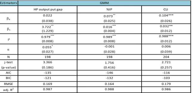
19 4.1 Baseline specification results
The Table II reports the results of our baseline specification (eq. 6) estimated through GMM with three different measures of output gap. At first glance, one may notice that the results are very sensitive to output gap measures. The results obtained from the standard HP output gap contradict those from the annual growth of the IP index and the annual growth of the
OECD composite leading indicator (CLI) (regardless of estimator used, see Annex A7).
The use of standard HP output gap provides us with statistically insignificant policy rate response to inflation gap (or even a negative response under OLS, see Annex A7), and points to a prominent role of the output gap in the monetary transmission mechanism due to its strong influences on future inflation (e.g., economic growth acceleration triggers a hike in the inflation expectation) – as also pointed in Gerlach and Smets (1999).
TABLE II: ESTIMATES OF TR IN THE EURO AREA: 1994:01-2011:12
Note: 1. Eq.6 : it = α + βπ (πt+6 - π )+ βxXt+3 + ρit-1 +εt Estimators 0.022 0.073** 0.104*** (0.038) (0.025) (0.026) 3.722** 0.016*** 0.032** (1.229) (0.004) (0.012) 0.979*** 0.989*** 0.988*** (0.008) (0.008) (0.012) 0.055* -0.001 0.006 (0.027) (0.028) (0.039) N 198 198 204 j-test 3.366 1.756 2.721 (p-value) (0.186) (0.416) (0.257) AIC -135 -146 -116 BIC -121 -132 -103 RMSE 0.169 0.164 0.179 adj. R2 0.987 0.988 0.986 GMM ρ βx α βπ
20
2. Standard errors in parentheses. *p < 0.05, ** p < 0.01, *** p < 0.001
3. AIC and BIC stands for the Akaike and Schwarz information criteria, respectively - the lower their value, the better the model; RMSE stands for root mean square error which measures the dispersion in the error term;
4. HP output put gap stands for the difference between the logarithm of the IP index and its Hodrick-Prescott-filtered
trend; %IP stands for the annual growth rate of the Industrial production index, and CLI for the annual growth rate of the amplitude adjusted composite leading indicator (CLIs) of the OCDE (see Annex A1);
5. The j-test stands for the Sargan-Hansen test, a test of overidentifying restrictions. The joint null hypothesis is that the instruments are valid instruments (uncorrelated with the error term). A rejection casts doubt on the validity of the instruments.
Contrary, when the economic activity is measured by the annual growth rate of the IP index or by the annual growth rate of CLIs, the policy rate response to the output gap, though statistically different from zero, is reasonably small in magnitude. Also, in these two cases, inflation gap appears to gain statistical relevance. According to these results, the ECB not only adjust the policy rate in response to inflation but also to the economic activity (conclusion not very distinct from those of Fourçans & Vranceanu (2004)).
The aforementioned observations support the ECB mandate for price stability, but none
of the specifications seems to fulfill the Taylor principle. Like in the Table 1, if we follow the
precept of the Taylor principle, it can be inferred that, the general small or no reaction to inflation gap might indicate a destabilizing behavior of the ECB (which is not realistic considering the ECB’s mandate). However, looking from other perspective, the small or no reaction to inflation gap might indicate the ECB’s success in anchoring inflation expectations, which caused inflation to be stable with small or insufficient variation regarding its target4. In fact, higher credibility of inflation targeting leads to less monetary policy response to changes in inflation (e.g., Peersman and Smets, 1999)
21
The relatively small magnitude in both inflation and output gap response coefficients may also be justified by the high degree of interest rate smoothing (ρ) and by the fact that the ECB considers a wide range of indicators of macroeconomic development other than inflation and output gap.
Concerning the policy rate response to its past values (ρ), it can be seen from the Table II
that ρ is robust and remarkably high, a common feature found across the different forms of TRs as noticed in the Table I (e.g., Clarida el al, 1998; Faust el al, 2001; among others), which points that the actual policy rate depends more on its past values that it does on the fundamentals. This monetary policy inertia suggests that only 3 to 4 percent of change in the interest rate is reflected in the policy rate within the month of change and that the rest will be adjusted in the remaining period. Therefore, rational agents should be able to anticipate future rates quite accurately.
Figure 1
In fact, as depicted in the Fig.1, ECB follows interest-rate smoothing in its monetary policy: ECB interest rates slowly fell from 3 to 2.5 percent then raised gain to 3 percent during 1999 and remained unchanged until 2000 when it gently rose to 4.75 percent, falling to 2
0 1 2 3 4 5 199 9M 01 199 9M 10 200 0M 07 200 1M 04 200 2M 01 200 2M 10 200 3M 07 200 4M 04 200 5M 01 200 5M 10 200 6M 07 200 7M 04 200 8M 01 200 8M 10 200 9M 07 201 0M 04 201 1M 01 201 1M 10
EBC 's Main Refinancing Rate
main refinancing rate
22
percent throughout 2003 and then remained unchanged for more than two years, starting smoothly ascending until 2008 when the ECB began to lower interest rates in response to the critical economic conjecture. Most recently, the ECB has cut interest rate to historically low level (0.75 percent in July 2012).
No matter the interpretation of ρ, it does enhance the fit of TRs: as it is removed from the regression, TRs show a significant departure from the actual interest rate with reasonable serially correlated errors (Fig.2 right side). From Fig.2 (left side), it can be seen that TRs track the ECB actual policy rate very closely – feature robust to all measures of the output gap,
independently of the estimator employed5. The major deviation of the actual policy rate from the
TR can be found in the interval encompassing mid-1998, the outburst of the financial crisis (mid-2007) and the ongoing Euro area sovereign debt crisis (mid-2009 – ).
Figure 2
These deviations can be seen not as ECB departure from a systematic behavior but an evidence of the need of some level discretion (or flexibility) in the implementation of monetary policy. The deviations from the TR correspond to crisis episodes (that impaired monetary policy
5 The chart associated to the OLS and LIML estimates are available on request.
0 2 4 6 8 1995m1 2000m1 2005m1 2010m1 mdate Eonia TR
Actual vs contrafactual policy rates
0 2 4 6 8 1995m1 2000m1 2005m1 2010m1 mdate Eonia TR
23
transmission channels) to which the ECB responded through non-standard measures (ECB, 2011, p.126-128).
The remarkably high adjusted R2 confirms the feature observed in the Fig.2, showing that, under the specifications used and regardless of output gap measures, TRs fit the actual data pretty well(except during economic turbulence period).
In terms of preferred specification, the information criteria the Akaike’s (AIC) and Schwarz's Bayesian (BIC) information criteria appear to reward the model in which the annual growth of the IP index is used as measure of the output gap. Intuitively, the annual growth of the IP index is not subjected to estimation uncertainty as the other two measures do, and hence, appears to be less misleading. Although the use of CLI produces better results regarding policy response to inflation, the model displays higher AIC. Therefore, in the rest of the paper the estimations will be based on the output gap measured by annual growth of the industrial production (IP) index.
4.2 Cross-checking different sample periods
In this section, the sample used covers the period which correspond to launch of euro area (January 1999) up to December 2011. The objective is to observe whether the use of unchained data displays major differences as compared to the chained pre-EMU and post-EMU data used so far (the estimation results are available in the Annex A8).
We observed a slight increase in the magnitude of the inflation response coefficient (βπ),
a decrease in magnitude and statistical significance of the output gap response coefficient (βx),
which asserts the ECB’s overriding mandate for price stability; and a slight decrease in the AIC
24
may tell us that though the ECB is more anti-inflationary than individual central banks of the
EMU member states, the national central banks cooperation and monetary policy coordinationin
the pre-EMU was indeed aimed at low inflation.
The βπ still does not exceed the value embodied in the Taylor principle. When the
expected realized output gap is removed from the TR (but included in the instruments set for inflation in the GMM estimator, as to reflect the ECB monetary policy mandate which does not respond directly to economic activity, but to its effects on inflation), βπ becomes statistically
very significant but still does not exceed a unit (results available in the Annex A9).
4.3 Change in the Economic Structure
Here we analyze the impact of the changes in the economic structure associated with the introduction of the single currency in 1999, the two more recent and severe financial crisis since the Great Depression, namely, the outbreak of the subprime crisis (August 2007) and the European sovereign debt crisis (November 2009), by considering dummy variables. In addition, given the results obtained, we also cross-check the TRs performance during subprime crisis period (2007:8-2009:06) and in the absence of it (by removing crisis period of time from the sample).
The dummies were set such that it takes on value 0 prior and 1 after January 1999, August 2007, and November 2009, respectively. The equation is depicted as follows:
(7) it = α + δD + βπ(πt+6 - π )+βxxt + ρit-1 + εt , where D stands for dummies.
The results concerning the inclusion of the dummies are reported in the table III. With regard to the introduction of the single currency in 1999, under the specifications being used,
25
apparently it did not triggered monetary policy response. This comes without surprise given the monetary convergence process (Maastricht Treaty or Criteria) that preceded the introduction of the single currency. This is in line with the results we obtained in the previous section.
As for the subprime crisis, the ECB appears to ignore it as the coefficient (dummy 2) shows up statistically insignificant, which may correspond to the fact that the ECB didn’t react aggressively to the subprime crisis at its outburst. This goes in line with Bouvet and King (2011), that found that August 2007 does not correspond to a structural break in the ECB policy (but December 2008, instead), given that the spillover effect of the US housing crisis on Europe started to feel severe only in the second half of 2008 (even though state interventions actuated offering liquidity to the banking system from the onset of the subprime crisis).
TABLE III: ESTIMATES OF TR IN THE EURO AREA: 1994:01-2011:12 DUMMIES FOR CHANGE IN THE ECONOMIC STRUCTURE
Note:
1. it = α + δD + βπ(πt+6 - π )+βxxt + ρit-1 + εt , estimated through GMM ;
2. Standard errors in parentheses (expect for the p-value). * p < 0.05, ** p < 0.01, *** p < 0.001;
3. Dummy1=0 prior and 1 after January 1999; Dummy2=0 prior and 1 after August 2007;and Dummy3= 0 prior and 1 after November 2009;
4. The output gap is measured as the annual growth in the industrial production index (%IP).
Dummy 1 Dummy 2 Dummy 3
δ -0.0292 0.00876 -0.0877* (0.061) (0.042) (0.044) βπ 0.0835 0.0817*** 0.0796** (0.048) (0.024) (0.028) βx 0.0153* 0.0154** 0.0155*** (0.006) (0.005) (0.004) ρ 0.984*** 0.991*** 0.978*** (0.015) (0.010) (0.012) α 0.0389 -0.00548 0.0426 (0.094) (0.045) (0.049) j-test 1.974 2.639 0.83 (p-value) (0.3726) (0.2672) (0.6604) N 198 198 198 adj. R2 0.987 0.987 0.988 GMM
26
In fact, it was not until October 2008 that the ECB Governing Council decided on interest rate cut by 50 basis points to 3.75 percent. The positive sign observed may be an indication of the increase in the policy rate carried out by the EBC in July 2008 on the basis of its assessment of risk to price stability.
Apparently the subprime crisis caused no change in the ECB’s behavior, so we cross-checked this outcome by both removing the financial crisis period from our sample and also restraining the sample to the crisis period6. In the first case, the policy response to both inflation
and output gap increases in magnitude and statistical significance. However, during the
subprime crisis, while policy response to output gap remains slightly the same, the response to inflation is rather statistically lower and has even a negative value. This may indicate that during the subprime crisis the focus of the ECB was not on inflation itself (variations appear to be perceived as temporary by the ECB, because long term inflation expectations are well-anchored), which by the way has been above 2 percent, but rather on factors that threat price stability (e.g., the economic activity). Also the interest rate smoothing coefficient, ρ, shows that monetary policy is more inertial in the absence of the crisis.
We also removed the output gap from the TR when working with the subprime crisis
sample (see footnote 6), and found that policy response to inflation, βπ, becomes very significant.
This outcome reinforces the important role of the output gap as leading indicators for inflation pressure.
As for the sovereign debt crisis (dummy 3) the result is consistent with the ECB dealing with it at its outburst through cuts in the interest rate.
27 4.4 Impact of additional explanatory variables
As we have seen, the relatively small magnitude in both inflation and output gap response coefficients, may also suggest that the ECB base its decision regarding the adjustment of the policy rate on a wide range of indicators of macroeconomic development, other than inflation and output gap. Therefore, following e.g., Clarida et al (1998), Gerlach and Schnabel (2000) among others, we extended the baseline regression by taking into account additional variables to widen the set of information to some extent. The regression is depicted as follows
(for the estimation results see AnnexA10)
(8) it = α + βπ(πt+6 - π )+βxxt + βγzt+ρit-1 + εt
where zt stands for additional explanatory variables such as federal funds rate; stock market
barometers, namely, Dow Jones Euro Stoxx, the DJ corrected for the economic activity growth, and the interest rate spread measure as the difference between the Euro area 10-year Government bond yield and 3-month euribor; exchange rates, both Real effective (REER) and Nominal effective (NEER) measure as annual change rates; monetary aggregate (M3) gap
measures as the deviation of M3 annual growth from the reference value (4½%) set by the ECB
(see Annex A1). In addition, regarding the role sovereign risk played in departures of policy from the rule we included Greek and Portuguese risk premiums measured as the difference between 10-year bond yield (Greece, Portugal) and 10-year Germany Government (“risk-free”) bond yield.
The results we obtained suggest that the predictive ability of many variables for future
28
is very responsive, given the existing financial flows links (a result that is contrary to Gerdesmeier and Roffia (2004) but consistent with Ullrich (2003)), the additional variables considered, appear to provide statically no additional information to the ECB governing council. However, they seem to have some economic significance, as we expect ECB to react to, for instance, a rise in the DJ euro stoxx by raising the policy rate, while lowering the policy rate in
response to hikes in the interest rate spread7. The sovereign risk premium (Greece, Portugal) is
only statically significant from August 2007 (only when both risk premiums are included in the regression simultaneously). The latter results may be related to ECB’s non-standard measures and the intervention of “Troika”8.
The result (from AnnexA10: βγ (M3)= -0.003) suggests that, though the M3 plays an
important role as a leading warning indicator of threats to price stability in medium to long term in the ECB monetary analysis, under the specification used (output gap measured by the annual growth in the IP index) the ECB policy rate is unresponsive to M3. This outcome is not uncommon in the TRs literature as e.g., Gorter et al (2008) and Gerlach and Schnabel (2000)
testifies. Also, this negative coefficient confirms the conclusions of Ullrich (2003), by which the
ECB follows a counterintuitive action regarding M3 growth, because, theoretically, we expect interest rate hikes in response to “harmful” money growth. Nevertheless, it does not imply that the growth of the M3 should be disregarded. As a matter of fact, monetary policy does not react
mechanically to deviations of M3 growth from the reference value9 .
7 See Annex B5 on https://www.dropbox.com/s/lz9qtw0ha5n7t73/AnnexB.pdf
8 The committee led by the European Commission(EC) with the ECB and the International Monetary Fund (IMF),
that organize and monitor loans to the governments of Greece, Ireland and Portugal.
29
In general, the output gap and inflation gap coefficient response, (βx) and (βπ)
respectively, continues to point out to the ECB’s overriding goal - price stability.
V.
CONCLUSION
This dissertation analyzes the capability of Taylor rules in tracking the ECB behavior from 1994:01 to 2011:12. Three different measures of output gap were employed and the TRs were estimated through GMM, following a simple forward-looking approach. The impact of the change in the economic structure associated to the launch of the euro, the outbreak of the subprime crisis and the subsequent European sovereign debt crisis on the course of the ECB’s policy-making were also analyzed. And finally, the TR was extended to consider the impact of additional explainable variables other than inflation and output gap.
It was found that policy rates response to either inflation or output gap is very sensitive to the output gap measure and estimation method: The standard Hodrick-Prescott output gap points to a prominent role of the output gap in the monetary transmission mechanism, which is consistent with the fact that economic growth is an indicator of risk to price stability. Contrary, when the economic activity measured by the annual growth rate of the industrial production (IP) index or by the annual growth rate of the composite leading indicator (CLIs), the general result suggests the ECB not only adjust the policy rate in response to inflation but also to the economic activity, even though their response coefficient are relatively small in magnitude.
Although the use of CLI (which components exhibit leading relationship with IP index at turning points) as proxy for the economic activity produces better result regarding the policy rate response to inflation gap, the model is penalized with higher Akaike’s (AIC) and Schwarz's
30
Bayesian (BIC) information criteria.
The empirical results also point to ECB unresponsiveness to the launch of the euro (January 1999) and to the subprime crisis at its outburst (August 2007). However, the sovereign debt crisis seemed to trigger an immediate response from the ECB. Results which are roughly consistent with observed ECB’s behavior.
With regard to the additional variables, our analysis suggests that the predictive ability of money and many other variables for inflationary pressure has weakened in recent years, showing no statistical significance.
We could see that, although simple, TRs seem to track the ECB policy decision very closely with major deviations occurring during the crises episodes. This close track is mainly caused by the gradualism of ECB monetary policy (attested by the high and robust degree of interest rate smoothing) and its systematic behavior. In fact, the outcome obtained points that the actual short-interest rate is heavily dependent on its own past values (fact which confirm the important role of credibility in the monetary policy). Despite of the close track, TRs may have little to say regarding all relevant information underlying the decision-making of the ECB.
For instance, none of the specifications employed fulfilled the Taylor principle and, in general, the coefficients obtained in our empirical results are quite small in magnitude. This may either be an evidence of a destabilizing behavior (according to the Taylor principle) of the ECB or of the ECB´s effort (through its two-pillar monetary policy strategy) to anchor inflation expectations which caused inflation to be stable with small variation regarding its target. Given the ECB’s anti-inflationary philosophy, it may be inferred that TRs or, more specifically, the Taylor principle is not in harmony with the reality of the actual ECB. This outcome calls for further and deepest research.
31
Because TRs are superficial representation of a complex reality, it does not cover all relevant information underlying the decision-making of the ECB. Nevertheless, due to it nature, TRs may still be used as an additional informative indicator.
VI.
REFERENCES
Albulescu, C.T. (2010), Forecasting Romanian Financial System Stability Using a Stochastic Simulation Model, Romanian Journal of Economic Forecasting, 13(1), 81-98.
Asso, P. F., Kahn, G. A., Leeson, R. (2010), The Taylor Rule And The Practice Of Central Banking, Federal Reserve Bank of Kansas City, Research Working Paper 10-05.
Belke, A. & Klose, J. (2010), How Do the ECB and the Fed React to Financial Market Uncertainty? The Taylor Rule in Times of Crisis, Ruhr Economic Paper 166.
Belke, A. & Klose, J. (2011), Does the ECB Rely on a Taylor Rule During the Financial Crisis? Comparing Ex-post and Real Time Data with Real Time Forecasts, Economic
Analysis & Policy, 41(2).
Bouvet, F & S. King (2011), Interest-Rate Setting At the ECB Following the Financial and Sovereign Debt Crises, In Real-Time, Modern Economy, 2(5), 743-56.
Brainard, W. (1967), Uncertainty and the Effectiveness of Monetary Policy, American
Economic Review, Papers and Proceedings, 57, 411-425.
Castelnuovo, E. (2007), Taylor Rules and Interest Rate Smoothing in the Euro Area, The
Manchester School, 75(1), 1-16.
Castro, V. (2011), Can Central Banks’ Monetary Policy be Described by a Linear (augmented) Taylor rule or by a Nonlinear Rule? Journal of Financial Stability, 7, 228-246.
32
Cecchetti, S. G., Genberg H., Lipsky J. & Wadhwani, S. (2000), Asset Prices and Central Bank Policy, Geneva: International Center for Monetary and Banking Studies 140.
Chow, G. & A. Lin (1971), Best Linear Interpolation, Distribution and Extrapolation of Time Series by Related Series, The Review of Economic and Statistics, 53(4), 372-375.
Clarida, R., J. Gali, & M. Gertler (1998), Monetary Policy Rules in Practice: Some International Evidence, European Economic Review, 42, 1033-1067.
Clarida, R., J. Gali, & M. Gertler (1999), The Science of Monetary Policy: A New Keynesian Perspective,” Journal of Economic Literature, 37, 1661-1707.
Clarida, R., J. Gali, & M. Gertler (2000), Monetary Policy Rules and Macroeconomic Stability: Evidence and Some Theory, Quarterly Journal of Economics, 115, 147-180.
Dotsey, M. (1998), The Predictive Content of the Interest Rate Term Spread for Future Economic Growth, Federal Reserve Bank of Richmond Economic Quarterly, 84(3). Elliott, G., T. Rothenberg, & J. Stock (1996), Efficient Tests for an Autoregressive Unit Root,
Econometrica 64, 813–836.
European Central Bank (2011), The Monetary Policy of the ECB, Third Edition, May, pp. 55-90.
Faust, J., J. Rogers & J. Wright (2001), An empirical comparison of Bundesbank and ECB
Monetary Policy Rules, Board of Governors of the Federal Reserve System
International Finance Discussion Papers 705.
Fourçans, A. & Vranceanu, R. (2004), The ECB interest rate rule under the Duisenberg presidency, European Journal of Political Economy, 20, 579–95.
33
Area, Swiss J Econ Stat, 140(1), 37–66.
Gerdesmeier, D. & Roffia, B. (2005), The Relevance of Real-Time Data in Estimating
Reaction Functions for the Euro Area, North American Journal of Economics and
Finance, 16(3), 293-307.
Gerlach, S. & Smets, F. (1999), Output Gap and Monetary Policy in the EMU area,
European Economic Review, 43, 801-812.
Gerlach, S. & G. Schnabel (2000), The Taylor Rule and Interest Rates in the EMU Area,
Economics Letters, 67, 165–171.
Gerlach-Kristen, P. (2003), Interest Rate Reaction Functions and the Taylor Rule in the Euro Area, European Central Bank, Working Paper 258.
Gerlach-Kristen, P. (2004), Interest-Rate Smoothing: Monetary Policy Inertia or Unobserved Variables? Contributions to Macroeconomics, 4, 1-17.
Gorter, J., Jacobs, J. & de Haan, J. (2008), Taylor Rules for the ECB using Expectations Data, Scandinavian Journal of Economics, 110(3), 473–488.
Marcellino, M. & A. Musso (2010), Real time Estimates of the Euro Area Output Gap: Reliability and Forecasting Performance, ECB Working Paper 1357.
Molodtsova, T., Nikolsko-R A. & Papell, D. H. (2011), Taylor Rules and the Euro, Journal
of Money, Credit, and Banking, 43 (2-3), 535-552.
Orphanides, A. (2001), Monetary Policy Rules Based on Real-Time Data, American
Economic Review, 91(4), 964-985.
Orphanides, A. (2003), Historical Monetary Policy Analysis and the Taylor Rule, Journal
of Monetary Economics, 50(5), 983-1022.
34
View from the Trenches, Journal of Money, Credit, and Banking, 36 (2), 151-75.
Orphanides, A. (2007), Taylor Rules, Federal Reserve Board Finance and Economics
Discussion Series 18.
Peersman, G. & Smets, F. (1999), The Taylor Rule: A Useful Monetary Policy Benchmark
for the ECB? International Finance, 2(1), 85–116.
Rudebusch, G.D. (2002), Term Structure Evidence on Interest Rate Smoothing and Monetary Policy Inertia, Journal of Monetary Economics, 49 (6), 1161-87.
Ruth, K. (2007), Interest Rate Reaction Functions for the Euro: Evidence from Panel Data Analysis, Empirical Economics, 38, 541-569.
Sauer, S. & Sturm, J. (2007), Using Taylor Rules to Understand European Central Bank Monetary Policy, German Economic Review, 8(3), 375-398.
Taylor, J. B. (1993), Discretion versus Policy Rules in Practice, Carnegie-Rochester
Conference Series on Public Policy, 39, 195-214.
Ullrich, K. (2003), A Comparison Between the Fed and the ECB: Taylor Rules, ZEW
Discussion Paper 03-19, Mannheim.
VII.
ANNEX
Annex A
Annex A1: Description of the variables and respective sources.
The ex-post data used in this exercise comprises monthly data covering the sample period 1994:01 to 2011:12, and refers to the Euro area - changing composition*. All the series are seasonally adjusted.
Variable Explanation Key
Source/re trieved on/Unit