UNIVERSIDADE DA BEIRA INTERIOR
Ciências Sociais e Humanas
On the nexus of energy use - economic
development: a panel approach
Jorge Fernando dos Santos Gaspar
Dissertação para obtenção do Grau de Mestre em
Economia
(2º ciclo de estudos)
Orientador: Prof. Doutor António Manuel Cardoso Marques
ii
Acknowledgements
I wish to express my sincere thanks to Professor António Cardoso Marques. I am extremely thankful and indebted to him for sharing expertise and encouragement extended to me. I also thanks to my family, especially to my parents, for the unceasing encouragement, supported me through this venture. I wish to thank my friends and colleagues for their support.
iii
Resumo
Considerando os desafios que se colocam à sustentabilidade do Planeta, está em curso um debate acerca do alvo crescimento económico versus desenvolvimento sustentável. O Produto Interno Bruto (PIB) tem sido o indicador usado para medir ambos, mas é ineficiente quando se trata de avaliar o desenvolvimento. Como alternativa considera-se o Índice de Bem-estar Económico Sustentável (IBES), o índice mais prominente avaliador do desenvolvimento. Este artigo compara os indicadores de desenvolvimento sustentável (IBES) e de crescimento económico (PIB), e a suas relações com o consumo de energia. A questão de investigação é: Os resultados evidenciados na literatura a propósito do nexus consumo de energia – crescimento económico serão sensíveis à consideração de outro indicador, mais fiel do desenvolvimento económico? Este trabalho testa as hipóteses tradicionais do nexus energia-crescimento através do estimador Panel-Corrected Standard Errors (PCSE), para um painel de 22 países num horizonte temporal anual compreendido entre 1995-2013. Foi usado o estimador PCSE pois foram detetados no painel fenómenos como dependência seccional, autocorreção e heterocedasticidade. Os resultados evidenciam importantes diferenças entre o IBES e o PIB no âmbito do estudo do nexus de energia. Verifica-se um efeito negativo do IBES no consumo de energia, assim foi descoberta uma nova hipótese negativa. A hipótese de feedback foi determinada para o PIB em relação ao consumo de energia. Para que se beneficie de desenvolvimento sustentável é necessário que os decisores políticos revejam a quantidade de energia consumida, a maneira como lidam com as trocas comerciais, os níveis ótimos de inflação e das taxas de juro. Assim sendo, devem ter em conta o IBES como indicador complementar do PIB e implementado globalmente. Isto deve intensificar o respeito pelos recursos naturais, aumentar o número de políticas referentes à eficiência de energia e melhorar o Bem-estar económico dos países.
Palavras-chave: Desenvolvimento Sustentável, Crescimento Económico, PCSE, IBES, Europa.
Palavras-chave
iv
Resumo Alargado
Hoje em dia é claro que o maior desafio que enfretamos enquanto especie prende-se com as alterações climáticas. O aumento de uma população cada vez mais consumista e satizfeita através da utilização de recursos naturais tem agravado o problema. O esforço para ultrapassar este desafio tem de ser global e como tal têm sido organizadas várias convençôes internacionais, das quais resultam medidas contra o problema. Apesar do que já foi feito ainda falta percorrer um longo caminho até os países começarem a crescer de forma sustentável, evitando o perigo das alterações climáticas. Um dos passos ainda por tomar é a forma como medimos o crescimento dos países, já que ainda utilizamos o Prodruto Interno Bruto (PIB) não podendo assim avaliar de que forma os países utilizam os recursos naturais que têm disponiveis, nem se tomam medidas que visam o crescimento sustentável e responsabilização dos danos feitos no ambiente. Nesse espirito tem surgido ultimamente na literatura o Índice de Bem-estar Económico Sustentável (IBES), que além de avaliar a pegada ecológica de cada país, ainda avalia o bem-estar económico, cobrindo assim várias areas, além da ambiental, em que os países têm de evoluir, tais como a pobreza e desigualdade na distribuição de rendimento. Sendo assim este trabalho foca-se na comparação entre o PIB e o IBES através do nexus de energia, já que o consumo de energia é o principal responsável pela exploração dos recursos naturais.
A literatura não é abundante quanto a estudos sobre o IBES, já quanto ao PIB e o nexus de energia é extensa destancando-se dela quatro hipoteses tradicionais: hipótese de feedback, hipótese de crescimento, hipótese de conservação e hipótese de neutralidade. Estas quatro hipoteses são testadas para os dois indicadores, comparando-se depois os resultados. O consumo de energia é ainda dividido em energias renováveis e energias de origem fóssil, permitindo, além de permitir avaliar o nexus de duas perspectivas diferentes, ainda é visto o impacto que estes dois tipos de energia têm no IBES e no PIB. Além do nexus de energia são ainda tidos em conta a diferença dos efeitos dos fatores economicos tradicionais, tais como tecnologia, inflação, investimento, abertura ao exterior e capital humano, nos dois indicadores estudados.
Foram utilizados vinte e dois países no estudo, todos aqueles que foram possíveis, já que se tratando de comparar indicadores macro-económicos, é de extrema importância que o maior número de países possível esteja envolvido. Pricipalmente tendo em conta a preocupação com as alterações climáticas, pois qualquer decisão tomada por um país que desrespeite gravemente o ambiente afecta todos. O horizante temporal considerado é de 1995 até 2013 de forma anual.
De forma a atingir o objetivo do estudo foi utilizada a base de dados em painel trabalhada com estimador Panel-Corrected Standard (PCSE), isto porque os testes Wald, Wooldridgde,
v
Pesaran, Frees e Friedman demonstraram heterocedasticidade, dependência entre “cross-sections” e autocorrelação contemporânea. Com a utilização do PCSE foram calculados quatro modelos, o 1º para avaliar o impacto dos fatores tradicionais de crescimento no IBES, o 2º averiguar se os mesmos fatores têm efeitos similares no PIB, o 3º com o principal objetivo de saber de que forma o IBES influência o consumo de energia e o 4º averiguar se o PIB têm impacto diferente no consumo de energia
Os resultados demonstram diferenças substanciais entre o IBES e o PIB. Em termos de nexus de energia foi descoberta uma nova hipótese conservativa negativa entre o IBES e o consumo de energia, já o PIB tem uma relação do tipo feedback. Quanto às energias renováveis foi descoberta apenas uma relação de crescimento com o IBES, tal como para as energias não renováveis com o PIB. Foi também visto que os fatores tradicionais de crescimento têm diferentes impactos nos dois indicadores estudados, entre eles a relação com a inflação, com o investimento e a abertura ao exterior. É assim concluído que para um desenvolvimento sustentável os países devem diminuir a energia consumida, principalmente nas cidades, rever os níveis ótimos de inflação e ter atenção ao tipo de trocas comerciais efetuadas. O IBES promove a aplicação de politicas de eficiência energética, o bem-estar económico e o respeito pelos recursos naturais. É importante que este índice seja implementado pelo maior número possível de países, evitando assim a movimentação de custos ambientais. Apesar disso o IBES é um índice mais apropriado para os desafios que a sociedade tem de enfrentar no futuro.
vi
Abstract
At a time when the major concern is the future of the planet, the debate of the distinction between growth and development is ongoing in scientific literature. Traditionally the Gross Domestic Product (GDP) is the indicator commonly used to measure both. However, it is very inefficient to evaluate development. The most prominent indicator as an alternative is the Index of Sustainable Economic Welfare (ISEW). The paper compares the sustainable development proxy (ISEW) with the economic growth measure (GDP), and their relation-ship with energy consumption. The research question is: The usual results for energy-growth nexus found in the literature change with a more suitable indicator to economic development? The traditional hypotheses of the energy-growth nexus are tested through Panel-Corrected Standard Errors estimator (PCSE), for a panel data that contains twenty-two Countries in annual data frequency for the time span 1995-2013. The PCSE is used because in the panel were detected cross-section dependence, serial correlation and heteroscedasticity. The results point out some differences between ISEW and GDP in the energy nexus. It was founded a negative effect from the ISEW on energy consumption, so a new negative conservative hypothesis was founded. The conservative hypothesis was proved for the GDP with energy consumption. It is also noted that for countries having sustainable development, policymakers should review the energy consumption quantity, the way that they manage the trade market, inflation and interested rates optimal levels. Therefore, policymakers should look at ISEW as complementary indicator to GDP and must be adopted by the most countries possible. This may intensify the respect for natural resources, increase the number of energy efficiency policies and improve countries economic welfare
Keywords
vii
Índex
1. Introduction 1
2. Measuring Sustainable Development 3
2.1. Measuring and comparing ISEW 5
3. Literature Review 11
3.1. Energy Nexus 11
3.2. Economic growth determinants 12 3.3. Energy consumption determinants 13
4. Data and Methodology 15
5. Results 17 6. Discussion 21 7. Conclusion 24 Appendix 26 References 27
viii
Figures list
Figure 1. Comparison between GDP and ISEW means in South and Central America Figure 2. Comparison between GDP and ISEW means in North America
Figure 3. Comparison between GDP and ISEW means in Asia. Figure 4. Comparison between GDP and ISEW means in Oceania. Figure 5. Comparison between GDP and ISEW means in Europe.
ix
Tables List
Table 1. ISEW components Table 2. Description of Models Table 3. Variables VIF values
Table 4. Specification tests for Model I and Model II Table 5. Specification tests for Model III and Model IV Table 6. Model I - Sustainable development
Table 7. Model II – Economic growth
Table 8. Model III - Energy consumption approached in a sustainable way Table 9. Model IV - Energy consumption approach in a traditional way Table 10. Pair-wise Granger causality tests
x
Acronyms list
BPSR BP Statistical Review CPI Consumer Price Index
ECOMPC Primary energy consumption per capita EEXPTPC Exported energy per capita
ENVTAXPC Environmental taxes revenue per capita EXPECTLIFE Expectancy life at birth
GDP Gross Domestic Product IEA International Energy Agency
ILOSTAT International Labour Organization Statistics IMPORTSPC Imports of goods and services per capita ISEW Index of Sustainability and Economic Welfare
NREPC Non-renewable energy sources consumption per capita OCDE OCDE Statistics
PATENTS Number of residential patents RENTSPC Natural resource rents per capita
REPC Renewable energy sources consumption per capita SAVINGSPC Savings per capita
SDGs Sustainable Development Goals TXEMP Employment rate
UN United Nations URBAN Level of urbanization VIF Variation Inflation Factor
1
1. Introduction
In 2015 was recorded the highest average temperature ever, which was a warning to the danger face by our planet at the moment and in the future. At same time World population is increasing. It currently stands at 7.3 thousand million, and is expected to increase 1.5 thousand million by 2030, causing the reborn of the possibility of the Malthusian trap (Malthus and Bonar 1965). To fight this, every country must decrease they environmental footprint. It is insufficient half of the countries starting have more respect for the environmental if the other half don’t do nothing. So since 1972 until 2015 in Paris, were organized several international meetings, every single one with insufficient results, but some with promising outcomes like the Sustainable Development Goals (SDGs).
One of the steps left to take is rethink the way we measure a country’s economic development, so that it becomes seen as an indication of the well-being provided by a nation and its efforts to ensure the planet’s future. Measuring only the consumption of goods and services, distribution and production processes is insufficient to evaluate countries’ sustainable development, defined as "development that meets the needs of the present without compromising the ability of future generations to meet their own needs" (WCED 1987).
The Gross Domestic Product (GDP) is the most used indicator to evaluate the sustainable development, however was recognized a long time ago as scarce by one of its creators (Kuznets et al. 1934). Is insufficient to measure the damage done to the environmental (Aşıcı et al. 2013) and is inefficient to quantify the society welfare (Costanza et al. 2009; Stockhammer et al. 1997). In view of this, the United Nations (UN) is naturally concerned with the use of the Earth’s resources and well-being. This has not only led to the drawing up of the 17 SDGs to this century, but also to concerns about measuring the well-being of countries and respect for the environment. This problem has been discussed more seriously, and there are several indices that measure social well-being, such as the Human Development Index and Gross National Happiness. However, only the Index of Sustainability and Economic Welfare (ISEW) created by Daly and Cobb in 1989, is established in the literature and includes the use of natural resources by each country. In addition, it takes into account factors such as inequality in income distribution, exchange of goods/services and investment in health or education by the Government. All this makes the ISEW the best indicator for measuring sustainable development, because it considers practically all the elements necessary to achieve the goals set by the UN as essential for the future of our planet and the generations who will live on it (Hák et al. 2016). These concerns are ignored in Gross Domestic Product calculating, the economic development proxy most used in scientific papers.
2
The ongoing world energy consumption growth is the biggest threat to a sustainable development (Oyedepo et al. 2014; M. Ozturk and Yuksel 2016). As is widely proven in the literature that a rise in energy consumption is related to economic growth (Bartleet and Gounder, 2010; Eggoh et al. 2011; Lise and Van Montfort, 2007), countries have lack of will to stop consumption. Following this line of thought, this paper compares the sustainable development proxy (ISEW), with the economic growth indicator (GDP), and examines the relationship of these two variables with energy consumption. The central question of this paper is: are the usual results of traditional energy-growth nexus (measured by GDP) valid when using a more suitable indicator for economic development, specifically the ISEW? Consequently, the paper’s main objectives are: (i) to assess the impact of energy consumption on sustainable development; (ii) to appraise the different effects on ISEW from renewable and non-renewable energies; (iii) to illustrate the differences between economic growth and sustainable development. For this purpose, annual data for twenty-two countries, covering the period from 1995 to 2013, was used. To achieve the main goals, micro econometric techniques were employed.
The results show the differences between using the ISEW and GDP to analyze the energy nexus. For ISEW is founded a new negative conservative hypothesis. Despite this hypothesis being new is proved very robust, however must be check in more detail. Energy produced by renewable sources is important to development as measured by the ISEW. However, one of the major drivers of GDP growth is the consumption of non-renewable energy sources, which makes the ISEW a better indicator to measure a country’s efforts to preserve the Planet.Also
some traditional economic growth factors have different effects in ISEW and GDP, such as inflation, trade openness and natural resources rents.
The reminder of this study is organized as follows: Section two explores the limitations of the way is measure the sustainable development, how ISEW can solve them and graphic comparison in 5 continents between ISEW and GDP; Section three provides the literature review about energy nexus, growth and energy consumption determinants; Section four describes data, the methods and the reasons to used them; Section five analyzes the empirical results; Section six present the discussion and Section seven the final conclusions.
3
2.
Measuring sustainable development
All indicators that estimate the economic development are proxies, because one single indicator cannot measure all the economy features. Then it is unlikely that GDP can measure correctly two different types of economic development such as economic growth and sustainable development. GDP arise as principal indicator in a post-world war II period, when was imperative a fast economic growth with peaceful international relationships. The indicator did his job, since it is a good way to look at the pace of the flow of goods and services, the consumption and the capital formation. However without looking at depreciation of the human, natural and social capital, the GDP growth, after a certain point, increases the income inequality and can reach the threshold point (Costanza et al. 2009; Max-Neef et al. 1995; Stockhammer et al. 1997).
Over time, GDP variation has been the country’s main concern, trying to increase it by the production and consumption of goods and services. Increasing economic activity has its costs, part of that are irreversible and others must be pay sooner or later. Rather sooner than later to avoid their accumulation like a debt between generations (Daly and Cobb, 1989). So a share of outputs of the production must be used to compensate the economy activity costs, so-called defensive costs. Just that way can be assured the same maximum consumption in a future period than in the current period, which is the main assumption of the Hicks income definition (Brennan et al. 2008; Hicks et al. 1946; Stockhammer et al. 1997).
In this paper the defensive costs taking into account in the ISEW construction (Table 1) are the income inequality with Gini Index, the natural resources depletion, the gross capital consumption and the inefficiency cost of the education and health public system. This defensive costs are part of the ISEW construction standard, thus decreasing the arbitrariness of their choice. The non-inclusion of the indicators like the cost of noise, cost of crime, cost of divorce or the non-intentional cars accidents, brings more liability to the statistics used. This kind of indicators is usually calculated from different ways in every countries and with lot of subjectivity. All the indicators used in this paper ISEW construction are withdraw from World Bank and ILOSTAT, removing calculation ambiguity (Table 1).
To the energy and mineral depletion calculation was used the resource rent method (El Serafy et al. 1997; Neumayer et al. 2000). It’s calculated the production profit discount in a 4 per cent rate until the resource end of life. The rate and the resources lifetime was defined by the World Bank taking into account that the profit decreases as the resource life time declines, mostly because resources became more difficult to extract. As the forest is a natural resource relativity easy to reset, they depletion calculation is done through the difference between forest exploration profit and reforestation. The damages caused by CO2
4
emissions are evaluate in 20 euros per ton by the World Bank, including the social cost which makes it different than they market value.
The unpaid work is included in the ISEW to accounting the welfare brought by unpaid domestic and volunteering work. The net capital growth is important to evaluate if the countries are formatting more capital than consume, thus satisfying the growing population with increasingly needs. The private consumption reveals the society wellbeing through families’ available income and is adjusted to Gini Index, because when rich families acquire more money create less welfare than the poor families (Daly and Cobb, 1989). As higher Gini Index value means more income inequality through society, is subtracted to one in the adjusted private consumption calculation.
This paper ISEW follows standard calculation to turn easier the adoption of this indicator as global. Other fact taking into account in the construction is the data available for the 22 countries. Given that the ISEW can be formally express as follows:
Where C is the private consumption adjusted to the GINI Index, G is the non-defensive public expenditures in health and education, K stands for net capital formation, N represents the natural environmental depletion and C represents the social defensive costs. As the last component is formed by different indicators in the several ISEWs and these indicators are calculated in different forms by each country, is difficult to study ISEW with social cost with panel data. Until the social costs having a standard calculation is almost impossible to ISEW contain this costs and became global. Therefore, ISEW in this study is formally express as follows:
This kind of formation can be seen in several ISEW studies, normally with social costs and with more environmental indicators, but just for one country (Gigliarano et al. 2014; Menegaki and Tsagarakis 2015; Pulselli et al. 2012). Due to lack of data there are few ISEW studies with panel data, standing out the Menegaki and Tugcu (2016) work that studies the Sub-Saharan Africa countries, also choosing exclude social cost from ISEW calculation. All this studies concluded that are substantial differences between ISEW and GDP, thus between sustainable development and economic growth.
5
Table 1. ISEW components
2.1. Measuring and comparing ISEW
The macro-economic indicators are very useful if they are used to compare countries, mainly when the indicator main objective is measure the sustainable development and the economic welfare. For this kind of indicators, the greater the number of countries used them, the more reliably they became. Which is even more evident for one indicator that measure negative externalities in the environment, damages that affect every country in the world and must be pay be someone. Taking into account this point of view, this paper studies every country with data available for the nine ISEW components formed by twelve indicators (Table 1). For a first comparison between ISEW and GDP, the countries were divided by continents to a more meticulous economic analyses and for take into account the regional economic changes. The only continent excluded from the study due to lack of data is Africa and the Mexico as single country from Central America was included in South America, because this economy evolution is more similar to the South America economies than to the North America economies.
The first comparison in this study is made between the ISEW per capita mean and the GDP per capita mean with a graph for each continent. The figure 1 demonstrates the difference
Component Data Source Computation
Adjusted private
consumption (+) Final household consumption expenditure – WDI Gini index – WDI
Final household consumption expenditure * (1- GINI Index)
Net capital
growth (+/-) WDI Gross Capital Formation - Gross Capital Consumption Health
expenditure (+)
WDI Public health expenditure * 0,5 Education
expenditure (+) WDI Public education expenditure * 0,5 Unpaid work (+) Number of unpaid workers-
WDI
Minimum wage – ILOSTAT
Number of unpaid workers * Average wage Mineral
depletion (-)
WDI Ratio of the value of the stock of mineral resources to the remaining lifetime reserve (capped at 25 years). It includes tin, gold, lead, zinc, iron, copper, nickel, silver, bauxite, and phosphate.
Net forest depletion (-)
WDI Calculated as the product of unit resource rents and the excess of round wood harvest over natural growth.
Energy depletion (-)
WDI Ratio of the value of the stock of energy resources to the remaining lifetime reserve (capped at 25 years). It includes coal, crude oil and natural gas.
Carbon dioxide
damage (-) WDI Carbon dioxide damage is estimated to be $20 per ton of carbon (the unit damage in 1995 in U.S. dollars) times the number of tons of carbon emitted.
Note: WDI, The World Bank- World Development Indicators; ILOSTAT, International Labour Organization Statistics;
6
between GDP and ISEW in South and Central America represented in the study by Brazil, Colombia, México, Chile and Peru.
Figure 1. Comparison between GDP and ISEW means in South and Central America The Gap between the two indicators started to be 627.58 dollars’ and increases until 2003, when ISEW reach is minimum value, where is 2977.324 dollars. Before the 2008 world crisis the gap is 2992.1 dollars, mostly because of the natural resources depletion that increases seven times is initial value (1995). With the crisis, the ISEW lost 13.8 % of its value and GDP “just” 2.4%, increasing again the gap between the two indicators, this trend goes on until the end (2013), reaching the 3244.7 dollars. As the countries studied in South and Central America were underdeveloped in 1995, they try to reach the rest of the world using them huge natural resources. Besides directly hit the ISEW, due to the damages done to the environmental, the gains with that exploration are unequally distributed through society. This continent has the lower ISEW value, because the economies from that region are based in the natural resources exploration, what causes same kind of “sustainable resource curse”. This happens when countries have many natural resources, naturally end up to explore them as possible, mostly when are less development countries, directing large part of the economy to activities that brings negativity externalities and social costs.
7
In North America were studied the two countries from this continent, the difference between the ISEW and GDP in that region can be seen in Figure 2.
Figure 2. Comparison between GDP and ISEW means in North America
The difference between the two indicators was 17322.13 dollars in 1995 and increases until 2000 to 20022.47 dollars, mainly because the adjusted private consumption just increase 7.7%, in this period, far from the approximately 17% who grew the two indicators studied. Which means that the increase of goods and services flow and capital formation was not reflected in available income of all society groups. In that period the capital was create mainly in tech enterprises, many overrated like was obvious in 2000s tech bust, causing 3% fall in the ISEW, however GDP rise around 0,3 % in that period. After the tech bust, the gap between the two indicators starts to diminish, reaching the 18660.5 dollars in 2007. With the world crisis, the ISEW lost 9% of this value, from 2008 to 2009, and GDP lost 3.8%. After that, the gap starts to diminishes again until 2013, where was 17985.98 dollars, but never reaching the minimum initial point in 1995. This continent is the one that starts with a major difference between the ISEW and GDP, because is formed only by Canada and the United States of America, two economies already developed in begging of the time span considered in the study. This difference does not expressively diminish, because these countries use the massive natural resources available and have structural problems related with the income distribution. The Canada has 0,665 like Gini Index mean during the time study and United States of America has 0,59, very high number for development countries
8
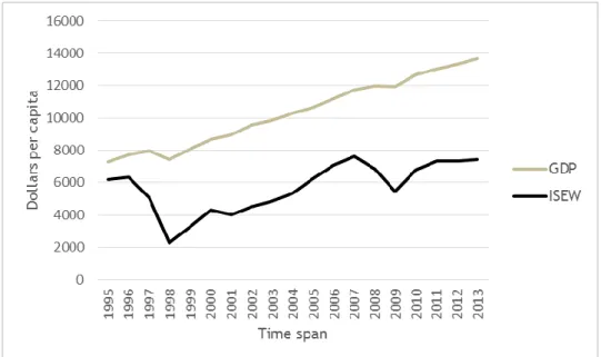
In Asia there was just two countries with available data for the ISEW construction, they were South Korea and Thailand. The differences between the two indicators studied in this paper for the two countries can be seen in Figure 3.
Figure 3. Comparison between GDP and ISEW means in Asia.
The ISEW value began to be just 1097.47 dollars less than GDP, but in 1997 this number starts to increase. In this year the Thailand government decided to stop the peg between the local currency (bath) and the dollar leading to a quick currency devaluation, causing exports revenues reduction and stock market declines. This crisis spreads throughout Asia, included South Korea, where banks stop to loan money at low interested rates, in the time when enterprises in Korea starts to expand. Therefore, the GDP, from 1997 until 1999, decreases 7.2% and ISEW loses 54.7% of this value. Despites the ISEW recovery, after the “Asia contagious” crisis, the gap between the two indicators never became as short. The world crisis brings other major ISEW depreciation, this time around 20 %, from 2008 to 2009, and GDP just fell 0.1%. While the first crisis had several structural damages, like Capital formation decreasing, the major effect of the second in the ISEW was in adjusted private consumption falling 10 %. Asia is the continent were crisis had more negative impact in ISEW, mostly due to characteristic markets deregulation from the region, then having many negative externalities, which are more explored in the “darkest times”.
9
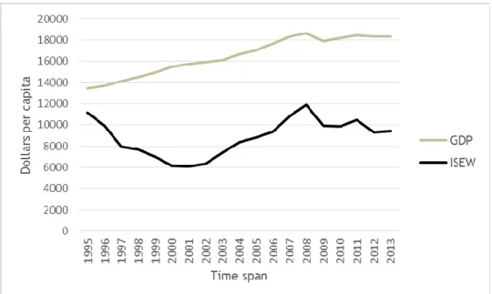
From Oceania this study contains also just two countries, Australia and New Zealand. In Figure 4 it can be seen the comparison between ISEW mean per capita and GDP mean per capita.
Figure 4. Comparison between GDP and ISEW means in Oceania.
The gap between ISEW and GDP in 1995 is 10903.42 dollars and increases until 2001, mainly because the adjusted private consumption diminished about 30 % in that period. This ISEW component is the most effective in this continent, because is value is around 60% of the ISEW value in the first years, reaching the 89% in 2012. The fact that this component being adjusted to Gini Index turns it even more important, since if Australia isn’t famous for their Gini value, (0.33 mean in the time span considered for developed country is not great), New Zealand has a serious problem of income distribution with 0.66 mean value in the studied period. Taking to account that one as Gini index value, means that all the income belongs to one person, the New Zealand Gini Index is one of the worst in the developed world. Saying that, it is normal that the gap between the two indicators remains the same or even increases, mainly with a global crisis like was seen in 2008, when ISEW from Oceania fell 16% and GDP just 1 %. After the crisis the all scenario changed, mostly because the measures taking by the governments to fight inequality, provided more income to the families. Thus this continent became the only one studied ending with lower gap between GDP and ISEW in 2013 than in the beginning of the considered time span (10092.37 dollars).
10
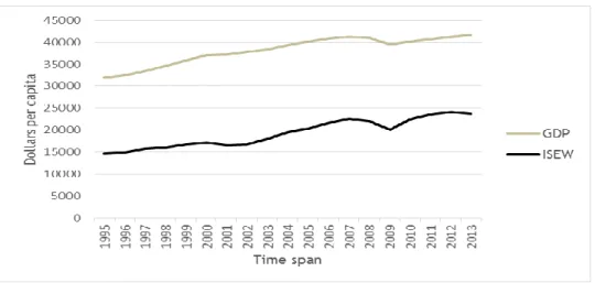
Europe was the region with more countries with available data, being they Portugal, Poland, Belgium, Russia, Ukraine, Slovakia, Romania, Netherlands, Czech Republic, France and Hungary. The difference between ISEW and GDP in that region can be seen in Figure 5.
Figure 5. Comparison between GDP and ISEW means in Europe.
The initial gap between the ISEW and GDP is just 2250.37, reaching the maximum value in 2002(9588.592 dollars). This major increasing happens due to the globalization effect seen in this period and widely proved in literature being linked to the income inequality growth (Asteriou et al. 2014; Bergh and Nilsson, 2010; Sheng et al. 2014). In addition to this, some European countries in this study were still underdeveloped and they were trying to reach the others countries development, mainly Russia and Ukraine that were trying by using them natural resources, which adversely affects the ISEW value. In the early 2000s the European countries studied start to have a more uniform growth, mostly because the entry in European Union by the less development countries like Romania, Czech Republic, Hungary and Slovakia. This brought to these countries more welfare and more suitable environmental standards, which was reflected by the ISEW growth in the early 2000s. The Gap between ISEW and GDP just starts to growth again with the world crisis in 2008, which leads the ISEW decreases 17.11% and GDP just 2.34%, from 2008 until 2010. The gap in 2013 was 8904.99 dollars, four times more than the initial gap registered in 1995.
11
3. Literature Review
There is a lack of empirical studies analyzing the nexus by focusing on development instead of economic growth, and few with comparisons of the ISEW and GDP (Beça and Santos 2014). The literature review to support this paper was divided into sections. The relationship between energy consumption and economic growth is presented in sub-section 3.1, the determinants of economic growth in 3.2.1, and energy consumption in 3.2.2.
3.1. Energy nexus
The causality relationship between economic growth and energy consumption has been widely explored, mostly by testing four hypotheses:
(i) The feedback hypothesis, in which energy consumption causes economic growth and vice versa. If this hypothesis is confirmed to ISEW it will mean that this indicator is fully dependent on energy consumption and energy efficient policies are harmful to sustainable development. The alternative to prevent the ongoing increase of the natural resources depletion, is promote the use of renewable energies, mainly if this hypothesis is settled to them. If this is the case the sustainable and economic welfare are fully dependent of renewables energies increasing. The same is true for the non-renewable energies and for economic growth. There has been a huge debate in the literature about the effects of renewables in economic growth, but few studies prove the feedback hypothesis in this relationship. As used of energy from non-renewables sources is based on resource depletion, it is unlikely that this hypothesis be proven between ISEW and non-renewables.
(ii) The neutrality hypothesis, which assumes that energy consumption and economic growth are neutral in regards to each other, meaning that energy efficiency policies can be used without production decreasing. Since is expected that the implementation of energy efficient policies does not affect the sustainable development, the neutrality hypothesis is likely to be confirmed. Energy consumption, particularity from the non-renewable resources, is one of the major factors to economic growth, having been widely proven in literature the positive link between the two (Apergis and Payne, 2012; Tugcu et al. 2012). Saying that, it is unlikely that this hypothesis can be settled with energy consumption and economic growth. This hypothesis is expected to be confirmed to the relationship between non-renewables and ISEW, due to the environmental damages that this kind of energy provokes. And to the renewables and economic growth, since it is not established in the literature that this kind of energy can increase production.
(iii) The growth hypothesis, which specifies a unidirectional relationship running from energy consumption to economic growth, therefore diminishing energy consumption affects economic growth. In Economies which GDP or ISEW depends on energy consumption are not
12
technological advanced enough or have an unappropriated legal frameworkto address energy flows. In economies like that, structural changes must take place to turn the economy receptive to energy efficient policies. With the methodology used in this paper, this hypothesis must be settled for the model I to sustainable development and for the model II to economic growth. There is many studies that established this hypothesis, mostly for the relationship between economic growth and energy consumption (Bowden and Payne, 2009; Kraft and Kraft, 1978; Stern et al. 2004).
(iv) The conservation hypothesis, which states a unidirectional causality implying that an increase in production causes an increase in energy consumption, but that economic growth is not fully dependent on energy consumption. If this hypothesis it will be confirmed, means that the economy of the countries is less dependent from energy consumption and closer to a sustainable economy. So this hypothesis it will be more likely to be proved with ISEW than with GDP, however several studies proved it using traditional energy nexus (Kraft and Kraft, 1978; Zhang and Cheng, 2009). For testing this hypothesis is computed the model III and IV, the first to demonstrate the connection from ISEW to energy consumption and the second the connection from GDP to energy consumption.
3.2. Economic growth determinants
The principal factors used in our study, which could potentially cause economic growth are labour, trade openness, inflation, energy, health and innovation. Due to lack of data, other factors like productivity and direct foreign investment were excluded from the study. Gross capital formation is an ISEW component and this precluded its use in the study. For trade openness, proxy imports per capita (IMPORTSPC) was used, which is widely proven to have a positive effect on growth, even in energy consumption studies (Al-mulali and Sheau-Ting, 2014). A higher value of imports per capita means more openness of the economy leading to better use for a comparative advantage in trade.
The employment rate is used as a labour proxy (TXEMP). A higher employment rate means more available income for more people, then is expected a positive effect in economic growth and in sustainable development. This variable is used in several energy nexus articles (Bowden and Payne, 2009; Ghali et al. 2004; Yildirim et al. 2012). All of these reach the same conclusion, i.e. a positive relation between employment and growth.
An important determinants of economic growth is inflation, represented in this study through the Consumer Price Index (CPI). One of the major targets to the policymakers is maintain the inflation levels inside certain limits, mostly to increase citizen’s purchasing power, thus increasing government popularity. However, the inflation management must be careful, because to much money supply has a negative effect in economic growth. The deflation and the stagflation phenomena are also dangerous to growth. Given that, in the literature,
13
inflation has a non-linear relation and is negative outside certain limits with Gross Domestic Product (Ibarra and Trupkin 2015).
Also tested in the study are the natural resource rents per capita (RENTSPC) from forests, oil, coal, and gas, allowing the valuation of the environmental impact for each country. Therefore, this determinant is essential to evaluate if ISEW is an indicator suitable to the environmental challenges that society faces, so a negative relation in ISEW is expected. The natural rents bring monetary advantages to the countries, therefore a positive relation with GDP is expected. However, can occur the natural resource curse effect due to the lack of diversification in resources used, which brings more exposure to external shocks, whether environmental or financial. On the other hand, an economy based on the export of resources leads, sooner or later, to an increase in foreign exchange rates, which brings a loss of competitiveness and subsequently, an economic crisis.
Part of the income is for consumption, the rest is for savings and turns into to investment. So savings per capita (SAVINGSPC) is used as a proxy for investment, which allows capital formation and so on economic growth. Then It is normal that savings as a determinant for economic growth has been widely studied, showing a positive effect (A. Ozturket al. 2015; us Swaleheen et al. 2008). The ability to save and invest leads to more available income and wellbeing grows, so is expected a positive relationship with ISEW.
The proxy of health is Expectancy life at birth (EXPECTLIFE) and also can show how capital accumulation can affect growth and sustainable development. Some studies demonstrate a non-linear relationship between EXPECTLIFE and growth, an invert U kind of association (Desbordes et al. 2011). Just turns in a positive linear relationship if the working day hours increase over time (Hickson 2009). With ISEW is expected a positive link, since people with higher longevity tends to have more concerns about future generations or/and they future, creating a concerned society (Frugoli et al. 2015; Mariani et al. 2010).
Technology innovation is measure through the number of residential patents (PATENTS). It is indicator of the innovation brought by a country society to the world. Technology innovation is the main factor responsible for having avoided that global capital depreciation overcame the capital formation throughout the ages. Thus countries could have economic growth without reaching the threshold point. Then it is usual be establish in the literature a positive relationship with economic growth and social welfare (Burhan et al. 2016; Niwa et al. 2016).
3.3. Energy consumption determinants
The principal primary energy consumption (ECOMPC) determinants seen in literature are the level of urbanization (URBAN), energy prices, GDP, the level of industrialization, taxation level and, less frequently, energy security. Levels of urbanization and industrialization have
14
been widely explored in energy studies with a consensual conclusion; they have a positive effect on energy consumption (Al-mulali and Sheau-Ting, 2014; York et al. 2003).
In this work, as pointed out previously, the consumer price index is used as a proxy for energy prices as it is in several other articles (Bartleet and Gounder 2010; Eggoh et al. 2011). Energy imports are used as the energy security proxy (Marques,Fuinhas and Manso, 2010). We predict that greater dependence on energy imports will lead to additional research into energy efficiency policies and will lead to a decrease in energy consumption. For energy exported (EEXPTPC) the opposite is expected. From RENTSPC is expect some kind of link, since more exploration of natural resources indicates easier access to them, increasing energy consumption. Is expected a negative from the environmental taxes revenue per capita (ENVTAXPC) on energy consumption, unless country already have reach the Laffer Curve fiscal critical point and the taxes rise no longer increase his revenues (Webster and Ayatakshi, 2013; Yin et al. 2016).
15
4. Data and Methodology
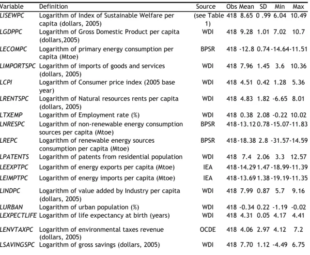
For the econometric models was used the same annual data, ranging from 1995 to 2013, for 22 countries around the world: Australia, Belgium, Brazil, Canada, Chile, Czech Republic, France, Hungary, Korea, Mexico, Netherlands, New Zealand, Poland, Portugal, Slovakia, United States of America, Colombia, Peru, Romania, Russia, Thailand and Ukraine. It was chosen taking into account the available data for the 12 indicators used to construct the ISEW (Table 1) and for the economic growth and the energy consumption determinants. The data sources, definition and descriptive statistics can be seen in Table 11 the Appendix.
An initial comparison was made between the ISEW and GDP by using a graph showing the evolution of each in five different continents (Sub-section 2.1). Then, to re-examine the energy nexus focusing on a sustainable approach, four panel data models were produced (Table 2), taking into account the growth determinants that affect economic growth and sustainable development at the same time. For an assessment of the traditional nexus hypotheses, a pair-wise Granger Causality test was performed to detect the direction of causality plus bidirectional relationships. The causality test was used between energy consumption (LREPC, LNREPC) and economic progress variables (LISEW, LGDPPC), with economic growth determinants as endogenous variables. Causality between primary energy consumption was also checked.
Table 2. Description of Models
All the variables are in natural logarithms to rescale the data and make the non-linear relations linear (L denotes natural logarithm before variable name). Data samples have been transformed into panel data form, which increases the number of observations, bringing higher viability to the study. Panel data can be performed under standard errors and residuals instability provided that the right estimators are chosen.
The Pesaran parametric test, the Friedman semi-parametric test and the Frees non-parametric test were carried out, all of them to random and fixed effects, in order to detect cross-section dependence. The Wooldridge test to identify serial correlation and the Wald modified test to recognize the group wise heteroscedasticity were also carried out. The used of four models with several explanatories each other can raise the suspicious of multicollinearity among them. Collinearity provokes loss of accuracy in the estimation of
Description Dependent variable
Model I Sustainable development LISEWPC
Model II Economic growth LGDPPC
Model III Energy consumption approach in a sustainable way LECOMPC
16
exogenous variables effects. To evaluate the presence of multicollinearity is compute the Variation Inflation Factor (VIF).
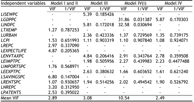
Table 3. Variables VIF values
As can be seen in the Table 3, the higher individual VIF value in Model I and II is 6.80 and the mean VIF is 2.89, in Model III the higher individual is 5.81 and the mean 3.08. No one reach the critical value 10, so is secure to ensure the nonexistence of multicollinearity. In Model IV (i), the mean VIF value is 10.54 and there are two individual values above 10, the LGDPPC (31.86) and the LINDPC (32.58) VIF values. There is linear dependence between them, so is made other model (IV) without LINDPC, since the presence of LGDPPC is essential to evaluate the energy nexus.
Independent variables Model I and II Model III Model IV(i) Model IV VIF 1/VIF VIF 1/VIF VIF 1/VIF VIF 1/VIF
LISEWPC LGDPPC - - - - 5.39 - 0.185426 - 31.86 - 0.031387 - 5.87 - 0.170303 - LINDPC - - 5.81 0.172018 32.58 0.030694 - - LTXEMP 1.27 0.787253 - - - - LURBAN - - 2.36 0.423336 1.37 0.729569 1.35 0.739175 LCPI LREPC LEXPECTLIFE 1.53 2.97 4.87 0.651993 0.337090 0.205365 1.11 - - 0.903319 - - 1.10 - - 0.907840 - - 1.08 - - 0.924071 - - LENVTAXPC - - 4.84 0.206416 2.91 0.343764 2.78 0.359508 LEIMPTPC LIMPORTSPC 1.76 - 0.568971 - 1.98 - 0.505956 - 2.27 - 0.439983 - 2.23 - 0.4477488 - LEEXPTPC LSAVINGSPC - 6.80 - 0.147004 2.63 - 0.380632 - 1.66 - 0.603652 - 1.61 - 0.621240 - LRENTSPC 1.07 0.930657 1.94 0.514256 2.02 0.494542 1.90 0.526792 LNREPC 3.20 0.312950 - - - - LPATENTS 2.53 0.395022 - - - - Mean VIF 2.89 3.08 10.54 2.49
Note: (i) Model not used in the study, with industrial level and GDP per capita included. The Model I and Model II VIF values are the same, since have equal independent variables. -, variables not used in the respective model.
17
5. Results
Besides the graphics seen in the sub-section 2.1, the comparison between the two indicators is also made through the energy-consumption nexus with panel data constituted by 22 countries. Due to the different characteristics of the countries seen in sub-section 2.1 different variations in economic growth are expected, which results in panel heteroscedasticity. Therefore, a modified Wald test was computed, where the null hypotheses is rejected, supporting the presence of heteroscedasticity. Panel data must be treated carefully, due the fact that they usually have complex error structures,therefore the Wooldridge, Pesaran, Free’s and Friedman tests were carried out.
Table 4. Specification tests for Model I and Model II
As it can be seen in Table 4 and Table 5 the modified Wald Test show evidence of group wise heteroscedasticity, through null-hypothesis rejection. With the rejection of null-hypothesis from the Wooldridge test was detected fist order autocorrelation. Only the null-hypotheses of Friedman test were not reject in model I, therefore was confirmed evidence of contemporaneous correlation across countries.
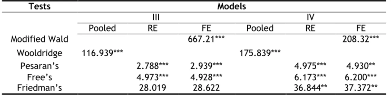
Table 5. Specification tests for Model III and Model IV
Results from the specification tests demonstrate contemporaneous autocorrelation, group-wise heteroscedasticity, and cross-section dependence for all four models. Coupled with the fact that FGLS is appropriate for panels with T>N and the panel used being constituted by 22 countries and 19 years, the PCSE is the most suitable estimator. In this way, four assumptions were tested for this estimator: one with first-order autocorrelation and a specific coefficient
Tests Models II II Pooled RE FE Pooled RE FE Modified Wald 2220.52*** 574.53*** Wooldridge 344.085*** 81.674*** Pesaran’s 2.588*** 2.686*** 13.062*** 12.237** Free’s 3.152*** 2.928*** 3.908*** 3.952*** Friedman’s 25.157 27.967 97.134*** 97.108*** Note: ***, **, *, denote significance level at 1, 5 and 10%, respectively.
Tests Models III IV Pooled RE FE Pooled RE FE Modified Wald 667.21*** 208.32*** Wooldridge 116.939*** 175.839*** Pesaran’s 2.788*** 2.939*** 4.975*** 4.930** Free’s 4.973*** 4.928*** 6.173*** 6.200*** Friedman’s 28.019 28.622 36.844** 37.372** Note: ***, **, *, denote significance level at 1, 5 and 10%, respectively.
18
AR (1) which is different for each country (Psar1); one with first-order autocorrelation but the same AR(1) coefficient for all countries (AR1); an independent (Ind) with unspecified autocorrelation but correlation over countries; and one with AR(1) common to all countries, and they resulted in heteroscedasticity level errors (Normal).
Model I (Table 6) shows the effects of economic growth determinants in LISEWPC. Thus it can be seen how traditional growth factors affect sustainable development.
Table 6. Model I - Sustainable development
Table 6 shows that only LRENTSPC are not statistically significant and it is kept in the table to reveal the differences with Model II. LPATENTS is not statistically significant with the Psar1 estimator, but significant with others. Model II (Table 7) was computed to understand the variations in economic growth in the time span considered. It also demonstrates the differences between effects on economic growth and sustainable development from the same determinants.
Table 7. Model II – Economic Growth
Independent variables OLS PCSE
Normal Psar1 AR1 Ind
LTXEMP 0.0929*** 0.0929*** 0.0934*** 0.0744** 0.0929*** LNREPC -0.1046** -0.1046** -0.1661** -0.0425 -0.1046** LREPC 0.0301*** 0.0301*** 0.0216** 0.0214** 0.0301*** LEXPECTLIFE 3.8040*** 3.8040*** 4.1211*** 4.0965*** 3.8040*** LCPI -1.0575*** -1.0575*** -0.9990*** -1.0105*** -1.0575*** LRENTSPC 0.0067 0.0067* -0.0080 -0.0107 0.0067* LIMPORTSPC 0.1713*** 0.1713*** 0.1591*** 0.1281** 0.1713*** LSAVINGSPC 0.5941*** 0.5941*** 0.6107*** 0.6031*** 0.5941*** LPATENTS 0.0270** 0.0270** -0.0003 0.0131 0.0270*** CONS -10.0356*** -10.0356*** -12.4206*** -10.3792** -10.0356*** N 418 418 418 418 418 R2 0.9190 0.9190 0.9951 0.9904 0.9190 Note: ***, **, *, denote significance at 1, 5 and 10% significance levels, respectively.
Independent variables OLS PCSE
Normal Psar1 AR1 Ind
LTXEMP 0.1369*** 0.1369*** 0.1726*** 0.1595*** 0.1369*** LNREPC 0.0973*** 0.0973*** 0.1400*** 0.2110*** 0.0973*** LREPC 0.0610*** 0.0610*** 0.0250*** 0.0186*** 0.0610*** LEXPECTLIFE 3.1740*** 3.1740*** 4.6032*** 5.0931*** 3.1740*** LCPI -0.4456*** -0.4456*** -0.1433*** -0.1171*** -0.4456*** LRENTSPC 0.0162** 0.0162*** -0.0018 -0.0043 0.0162*** LIMPORTSPC 0.2225*** 0.2225*** 0.2585*** 0.2392*** 0.2225*** LSAVINGSPC 0.3998*** 0.3998*** 0.2171*** 0.1629*** 0.3998*** LPATENTS 0.0266** 0.0266** 0.0081 0.0234** 0.0266** CONS -5.1944*** -5.1944*** -11.5547*** -12.4569*** -5.1944*** N 418 418 418 418 418 R2 0.9433 0.9433 0.9974 0.9935 0.9433 Note: ***, **, *, denote significance at 1, 5 and 10% significance levels, respectively.
19
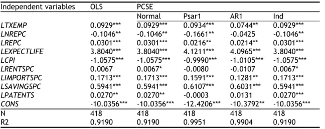
Model II show robustness with almost all variables except for LRENTSPC, not significant in AR1 and Psar1 estimators. Model III (Table 8) shows how energy consumption determinants affect this, mainly the LISEWPC.
Table 8. Model III - Energy consumption approached in a sustainable way
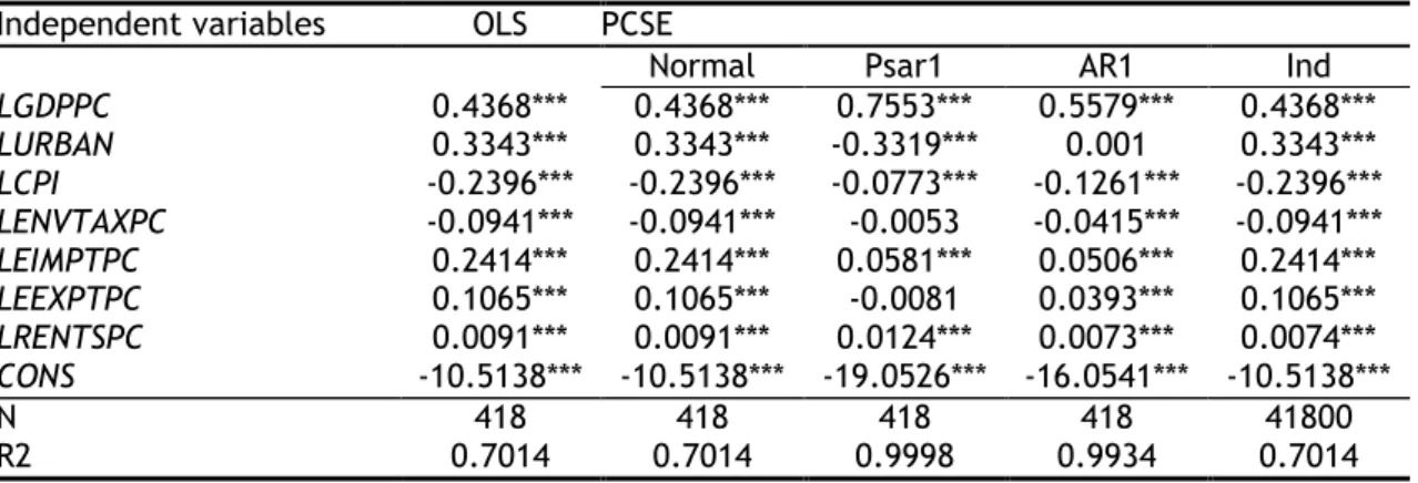
Model III is robust with almost all variables. Model IV (Table 9) is computed with the same variables excluding LISEWPC and adding GDPPC, to demonstrate the different effects of the two indicators on energy consumption. In comparison with Model III, LINDPC is excluded due to existence of multicollinearity with LGDPPC, which could have skewed the results.
Table 9. Model IV - Energy consumption approach in a traditional way
Table 9 shows that model IV is robust and that LGDPPC has a different effect on energy consumption than LISEWPC. Next, pair-wise Granger Causality was performed to analyze the traditional energy nexus and the energy nexus with LISEWPC as a proxy for sustainable development. So the two different nexuses can be compared.
Independent variables OLS PCSE
Normal Psar1 AR1 Ind
LISEWPC -0.1322** -0.1322*** -0.0286 -0.0345 -0.1322*** LINDPC 0.5783*** 0.5783*** 0.7766*** 0.5774*** 0.5783*** LURBAN 0.4011*** 0.4011*** 0.0186 0.1377 0.4011*** LCPI -0.3115*** -0.3115*** -0.1245*** -0.1466*** -0.3115*** LENVTAXPC -0.0856*** -0.0856*** -0.0083 -0.0355*** -0.0856*** LEIMPTPC 0.2652*** 0.2652*** 0.0777*** 0.0711*** 0.2652*** LEEXPTPC 0.1101*** 0.1101*** 0.0257*** 0.0484*** 0.1101*** LRENTSPC 0.0091*** 0.0091*** 0.0124*** 0.0073*** 0.0074*** CONS -9.2432*** -9.2432*** -16.9531*** -14.6561*** -9.2432*** N 418 418 418 418 41800 R2 0.6889 0.6889 0.9994 0.9925 0.6889 Note: ***, **, *, denote significance level at 1, 5 and 10%, respectively.
Independent variables OLS PCSE
Normal Psar1 AR1 Ind
LGDPPC 0.4368*** 0.4368*** 0.7553*** 0.5579*** 0.4368*** LURBAN 0.3343*** 0.3343*** -0.3319*** 0.001 0.3343*** LCPI -0.2396*** -0.2396*** -0.0773*** -0.1261*** -0.2396*** LENVTAXPC -0.0941*** -0.0941*** -0.0053 -0.0415*** -0.0941*** LEIMPTPC 0.2414*** 0.2414*** 0.0581*** 0.0506*** 0.2414*** LEEXPTPC 0.1065*** 0.1065*** -0.0081 0.0393*** 0.1065*** LRENTSPC 0.0091*** 0.0091*** 0.0124*** 0.0073*** 0.0074*** CONS -10.5138*** -10.5138*** -19.0526*** -16.0541*** -10.5138*** N 418 418 418 418 41800 R2 0.7014 0.7014 0.9998 0.9934 0.7014 Note: ***, **, *, denote significance level at 1, 5 and 10%, respectively.
20
Table 10. Pair-wise Granger causality tests
LISEWPC LPIBPC LCEPRIM LREPC LNREPC
LISEW does not cause - - 9.45*** 0.228 8.791***
LPIBPC does not cause - - 7.3778*** 0.232 0.239
LECOMPC does not cause - 6.151** 0.107 - -
LREPC does not cause 3.412* 0.165 - - -
LNREPC does not cause 0.395 3.094* - - -
Note: ***, **, *, denote significance level at 1, 5 and 10%, respectively
The pair-wise Granger tests demonstrate that the direction of causality between the endogenous variables used are; LREPC→LISEWPC; LNREPC→LGDPPC; LECOMPC←LISEWPC; LECOMPC ↔ GDPPC; and LNREPC → LISEWPC.
21
6. Discussion
The graphics from sub-section 2.1 shows different trends between GDP per capita and ISEW per capita from 1995 until 2013. In development countries, like in Oceania and North America, the two indicators diverge, mainly due to income inequality growing and private consumption decreasing. In less development countries, like in South, Central America and part of Europe, the difference between GDP and ISEW becomes bigger over time, when these countries were trying to development taking advantage from the natural resources, thus losing environmental standards. Every single financial crisis like the tech bust, “Asia contagious” or the world more effective in 2008, affects more the ISEW value than GDP value in every continent. Which proves that countries are willing to sacrifice the society wellbeing and losing the respect for the environment to have best financial results and having a higher economic growth. It was also noticed that in almost every continent, except for Oceania, the gap between GDP and ISEW increased during the time span studied. Meaning that the financial benefits from the economic growth are worse distributed through society and that growth is achieved causing bigger damages to the environmental. Which even cannot mean that countries are using more natural resources, but at least the resources are much scarcer, since is used the resource rent method in ISEW calculation, the decline came about them. Following economic theory, inflation, represented by LCPI in the model, has a negative effect on economic growth, mainly outside certain limits. In this study, this effect is stronger in ISEWPC, because when prices rise, increased production follows, leading to pressure on natural resources, less respect for the environment and losses in real income available. The limits for “good inflation” seem to be more restricted for sustainable development than for economic growth.
The incentives and ability to save, which defines the savings level, naturally has a positive influence on the two indicators studied. It is more effective in ISEWPC, because higher level of savings implies less consumption, which is the major cause of pressure on natural resources. Optimal interest rates should be redefined to promote sustainable development in the future. It is also important promote green investments, adopting “green Keynesian policies”.
Employment rate and expectancy life have the expected positive effect in ISEWPC and GDPPC. Higher employment rate means more people with additional income available, which brings more welfare to society and increase consumption, therefore brings higher flow of services and services, measured by GDPPC. A greater expectancy life at birth demonstrate a better health system, one of the most important facts to countries development. Besides welfare, is also a positive fact to the environment, since people with higher longevity tends to have more concerns with it.
22
In Model I and II the innovation has a positive sign, which is normal, since is a very important fact to human evolution. The effect of patents registered by residents is more robust in GDPPC than in ISEWPC. This is comprehensive due the fact that not every patents registered bring welfare or contribute to a resources efficient use. Patents of low technical merit and the “patenting in time strategy” used by enterprises leads to more consumption of goods and services but reduce competition, increasing prices, therefore diminishing welfare society. Imports of goods and services have an effect in models 1 and 2, showing the importance of open trade. In the case of the ISEW, this still has the effect that liberalized trade can shift polluting activities from developed countries with higher production cost, such as environmental taxes, to poorer countries. The influence is even stronger in GDPPC, which turns the race-to-the-bottom theory more likely. This theory states that after countries open up to trade, they prefer to adopt looser standards of environmental regulation in order to gain international competitiveness.
The increase of the money won with rents from natural resources (RENTSPC) has a different effect in GDPPC than it has in ISEWPC. The positive and significant effect in GDPPC it’s normal due to the profitability of resources exploration. The non-significant effect in ISEWPC is evidence of a “sustainable resource curse”. The money gain trough natural resources exploration activity is not enough to cover the environmental costs and still bring welfare to society. Which means that environmental costs are very high and the profits from natural resources activities are inequality distributed through society.
A negative effect can be seen for non-renewables energies with the ISEW, but increases in renewable energy sources consumption implies growth in the ISEW (growth hypotheses), the last was confirmed by the pair-wise Granger tests. So using the ISEW as an indicator, the choice between renewable and non-renewable energy becomes clear. The effect from non-renewable energy sources in GDP is stronger than the non-renewable energy sources, which is confirmed by the pair-wise Granger tests. So a decrease in non-renewable energy consumption provokes a higher reduction in production.Due this fact it is understandable why governments continue to invest in non-renewable energy.
The effects of IMPORTSTPC, RENTSPC, REPC and NREPC in GDPPC/ISEWPC, proves that internal production, mainly using natural resources, diminishes the chances of a sustainable development but increase economic growth. To achieve sustainable development, countries can stay with the production of goods and services, just have to find better way to produce them, for example with renewable energy sources. It is important that countries follow that pathway and stop to import from countries with lower environmental standard values. Therefore, the possible ISEW adoption as macroeconomic indicator has to be global with a standard calculation. Thus avoiding transfers from environmental costs by ISEW adopters’ countries to the others with “anything to loose”.
23
Models 3 and 4 confirm that energy prices have a negative effect on energy consumption,due to CPI and ENVREVPC effects, the last confirming the effectiveness of taxes on consumption. The EEXPTPC and RENTSPC confirmed that countries with energy production can get energy cheaper and easier, thus increasing the consumption. The rise of urbanization level brings all the energy consumption associated to the cities. The level of industrialization is important too. Energy consumption grows with increased energy imports, which suggests that countries are looking for better prices abroad, and not just for local production, which is more expensive.
The industrialization level is excluded from model IV, because is linearly dependent from GDPPC, indicating that they are a good proxy from each other. From this fact is concluded that GDP can demonstrate with reliably the evolution of industrial production. Without taken into account the costs from this activity, manly the damages provoked in the environment and well-fare. Then it was predictable the positive effect from the INDPC on ECONPC in Model III.
The unexpected energy imports positive effect in energy consumption can be explained by the fact that energy prices, even including profit production, political and social instability effects, is still cheaper than increase energy production and so leads to more consumption. Taken into account that mostly of energy imports is from fossil is easy to conclude that the renewable energy is still very expensive.
The feedback hypothesis was determined by Granger causality between GDP and total primary energy consumption. Economic growth is dependent on energy consumption, as seen in model 4 in a positive way. So, to become richer, more energy consumption is necessary, which at a certain point in the future, will be impossible. For the ISEW and energy consumption, the conservation hypothesis was determined, but with a negative effect, as seen in model 3. So is settle a new hypothesis in nexus, an increase in the ISEW provokes a decrease in energy consumption. Diminishing energy consumption can lead to sustainable development. Therefore, Model III and IV sets out same tips to policymakers make “sustainable decisions”. The higher positive coefficient affecting the energy consumption in the two models is from urbanization level, so is essential turn cities sustainable, with policies like making green buildings, electrifying transports and increasing green spaces. The Industrial level also has an important effect in energy consumption. One of the policies that can solve this problem is the rise of environmental taxes as results proved by Model III and IV. This kind of fiscal policy must be carried out with caution and idealistically must be global to avoid industries relocation to other countries taking advantage of facilities in green taxation.
24
7. Conclusion
In this paper, panel data techniques were applied, namely the PCSE estimator, to study the traditional energy growth-nexus from a perspective of sustainable development. As such, two alternatives were compared, the ISEW and the GDP for a set of twenty-two countries for a time span from 1995 to 2013. Beyond the nexus evaluation, the comparison is made through measuring the effects of economic growth in the two indicators. It’s also made two more models measuring the effects of energy consumption determinants and the pair-wise Granger tests to verify the nexus bidirectional hypothesis.
The findings prove that the conclusions reached using the traditional energy consumption-economic growth nexus are quite different from those obtained using the ISEW. The growth hypothesis was determined for the ISEW with renewables and for GDP with non-renewables. In turn, the feedback hypothesis between GDP and energy consumption was confirmed. Moreover, there was a negative effect from the ISEW on energy consumption, so a new conservation negative hypothesis was settled. This hypothesis is absent from traditional growth nexus, but very robust in this paper, however must be check by more studies in more detail.
Despite the focus of comparison between sustainable development (ISEW) and economic growth (GDP) in energy nexus, this study shows more important differences between the two. The econometric sustainable model compute suggests lowers inflation and interested rates than the classical optimal levels in economic growth model. The financial gains fail to cover the environmental costs and create enough welfare, evidencing a “sustainable resource curse”. For countries is still more financial rewarding import energies than the renewables own production. With different effects from trade dynamics in GDP than in ISEW and the rising globalization, this new indicator has to be adopted for all countries. Thus avoiding the competitive advantages gains and environmental costs transfers to countries with poorer environmental standards.
This paper sheds some light on the risk that a traditional interpretation of the energy-growth nexus could lead policymakers to make decisions that compromise the sustainable future, such as policies that indefinitely increase energy consumption. It’s one of the reasons for the countries studied being far from a sustainable development pathway. For change it, policymakers must promote energy efficiency policies, manly in industry and cities, like electrifying transports, stimulate renewables energies production and green buildings. These policies can be financing by standard green taxation for the greatest number of countries possible.
25
The global ISEW adoption as macroeconomic indicator can lead policymakers to implement energy efficiency policies, have more respect to natural resource and increase society wellbeing. GDP is a suitable indicator to measure financial variations but ISEW is more appropriated to the challenges faced by the society in the future.