Revisiting fiscal sustainability: panel cointegration and structural breaks in OECD countries

Carlos Pestana Barros & Nicolas Peypoch

A Comparative Analysis of Productivity Change in Italian and Portuguese Airports

WP 006/2007/DE _________________________________________________________

António Afonso & João Tovar Jalles

Revisiting fiscal sustainability: panel cointegration

and structural breaks in OECD countries

WP 29/2012/DE/UECE _________________________________________________________

De pa rtme nt o f Ec o no mic s

WORKING PAPERS

ISSN Nº 0874-4548

School of Economics and Management

Revisiting fiscal sustainability: panel cointegration

and structural breaks in OECD countries

*

2012

António Afonso

and João Tovar Jalles

Abstract

We assess the sustainability of public finances in OECD countries, over the period 1970-2010, using unit root and cointegration analysis, both country and panel based, controlling for endogenous breaks. Results notably show: lack of cointegration – absence of sustainability – between government revenues and expenditures for most countries (except for Austria, Canada, France, Germany, Japan, Netherlands, Sweden, and UK); improvements of the primary balance after past worsening in debt ratios for Australia, Belgium, Germany, Ireland, Netherlands and the UK; Granger causality from government debt to the primary balance for 12 countries (suggesting the existence of Ricardian regimes). Overall, fiscal policy has been less sustainable for several countries, and panel data results corroborate the time-series findings.

JEL: C32, E62, H62, H63

Keywords: debt, primary balance, fiscal regimes, stationarity, breaks, causality, panel cointegration, FMOLS

_____________________________

* _{The authors are grateful for comments from Artur Lopes, and from participants at ECB and at ISEG/UTL seminars, and to}

Roberta De Stefani for research assistance. The opinions expressed herein are those of the authors and do not necessarily reflect those of the ECB or the Eurosystem.

$ _{ISEG/UTL - Technical University of Lisbon, Department of Economics; UECE – Research Unit on Complexity and}

Economics. UECE is supported by FCT (Fundação para a Ciência e a Tecnologia, Portugal), email: aafonso@iseg.utl.pt.

# _{European Central Bank, Directorate General Economics, Kaiserstraße 29, D-60311 Frankfurt am Main, Germany. email:}

antonio.afonso@ecb.europa.eu.

+ _{University of Aberdeen, Business School, Edward Wright Building, Dunbar Street, AB24 3QY, Aberdeen, UK. email:}

j.jalles@abdn.ac.uk

# _{European Central Bank, Directorate General Economics, Kaiserstraße 29, D-60311 Frankfurt am Main, Germany. email:}

Contents

Non-technical summary ... 3

1. Introduction ... 4

2. Theoretical Framework ... 6

3. Econometric Methodology ... 9

3.1. Time series ... 9

3.2 Panel Data ... 13

4. Empirical Analysis ... 15

4.1 Stylised Facts and Data Overview ... 15

4.2 Country Analysis ... 19

4.3 Panel Analysis ... 22

5. Conclusion ... 25

References ... 26

Appendix A ... 31

Non-technical summary

The importance of sustainable public finances has received increasing attention particularly in the context and following the 2008-2009 economic and financial crisis. Sustainable fiscal policies can be continued indefinitely without any change in the policy stance, and when the intertemporal government budget constraint holds in present value terms. Conversely, if budgetary imbalances prevail, economic policies at both macro and microeconomic levels will quickly become unsupportable and changes would be required. If such a phenomenon occurs, then fiscal imbalances would imply a need for larger and more painful adjustments for the economy.

The main purpose of this paper is to investigate and draw some policy lessons on the sustainability of fiscal policy in a set of 18 OECD countries, using annual data over the period 1970-2010. Besides answering this policy question, we are also interested, among other things, in ascertaining the causal direction between government expenditures and revenues. The causal direction between the two budgetary variables may provide useful insights into how policy makers can manage budget deficits in the future. In our empirical approach we perform a systematic analysis of the stationarity properties of the first-differenced stock of government debt as well as, on the one hand, the relation between government revenues and expenditures and, on the other hand, the relation between primary balances and debt. These approaches provide us with an indirect test on the solvency of public finances in these countries. We conduct this analysis on a country-by-country basis, by means of several time series techniques, for robustness purposes, as well as for the country panel as a whole.

Our contributions are as follows: i) we combine both individual-country analysis by means of (recent) time-series techniques with panel data approaches for completeness and robustness purposes; ii) we take a longer time span and make use of uniform and comparable data for 18 OECD countries; iii) and we explore three different channels to evaluate fiscal sustainability as put forward in theoretical terms, that is, by looking at the first-differenced debt ratios, the relationship between government revenues and expenditures and, finally, the relationship between (lagged) public debt and primary balances.

Our results show that the first-differenced debt series for most countries is non-stationarity suggesting that the solvency condition would not be satisfied. Moreover, evidence suggests the existence of one cointegrating relationship in only 6 countries between revenues and expenditures. However, the overall test results allow the rejection of the cointegration hypothesis in both relationships under scrutiny. In other words, government expenditures, in half of the countries, exhibited a higher growth rate than government revenues, challenging therefore the hypothesis of fiscal sustainability.

On the other hand, the cointegrating coefficients for the revenues-expenditures relationship are positive (but less than one) and statistically significant, meaning that for each percentage point of GDP increase in public expenditures, revenues increase by less than one percentage point of GDP. In terms of causality, our evidence suggests stronger effects running from revenues to expenditures and most countries are not able to generate the revenues required to finance the planned expenditures. We find Granger-causality from government debt to the primary balance, which can be seen as evidence of the existence of a Ricardian regime.

1. Introduction

The importance of sustainable public finances has received increasing attention particularly in the context and following the 2008-2009 economic and financial crisis. From a fiscal perspective, maintaining a stable long-term relationship between expenditures and revenues is one of the key requirements for a stable macroeconomic environment and a sustainable economy. Therefore, our purpose is to find out whether fiscal imbalances in a number of OECD countries need to be curtailed before they become economically unsustainable, leading to insolvency situations.

Sustainable fiscal policies can be continued indefinitely without any change in the policy stance, and when the intertemporal government budget constraint holds in present value terms.1 Conversely, if budgetary imbalances prevail, economic policies at both macro and microeconomic levels will quickly become unsupportable and changes would be required. If such a phenomenon occurs, then fiscal imbalances would imply a need for larger and more painful adjustments for the economy. Given the detrimental impact of persistent deficits, practices on debt sustainability and appropriate fiscal policies are extremely important. For instance, Blanchard et al. (1990) present as a definition of a sustainable fiscal policy one that allows, in the short-term, that the debt-to-GDP ratio returns to its original level after some excessive variation.

There has been a substantial volume of empirical studies focusing on fiscal sustainability, tackling explicit government liabilities, looking notably at the US and European cases (see, Hamilton and Flavin, 1986; Hakkio and Rush, 1991; Trehan and Walsh, 1991; MacDonald, 1992; Ahmed and Rogers, 1995; Quintos, 1995; Makrydakis et al., 1999; Feve and Henin, 2000; Martin, 2000; Bravo and Silvestre, 2002; Hatemi-J, 2002; Afonso, 2005, Mendoza and Ostry, 2007; Arghyrou and Luintel, 2007; Afonso, 2008; Afonso and Rault, 2010; Afonso and Jalles, 2011, to name a few). In particular, Trehan and Walsh (1991) and Afonso (2008) are of interest in what follows since they emphasize the relationship between primary balances and government debt. In addition, Fincke and Greiner (2011), and Legrenzi and Milas (2011) focus on the possibility of finding structural breaks or possible non-linearities notably vis-à-vis debt thresholds, also in a fiscal reaction approach.2

_____________________________

1 _{Analysis on fiscal sustainability has focused on both the univariate properties of government debt (e.g. Hamilton}

and Flavin, 1986) and on the long-run relationship between government revenues and expenditures (e.g. Hakkio and Rush, 1991).

2 _{Regarding the specification of fiscal reaction functions, not the main purpose of the current paper, Afonso and}

On the other hand, Bohn (2007) provides a substantial challenge to the time series literature on fiscal policy. Specifically, Bohn suggested that rejections of stationarity-based sustainability tests are invalid because in an infinite sample, any order of integration of debt is consistent with the transversality condition which implies that the intertemporal budget constraint may be satisfied even if these particular time series tests are not. Instead, Bohn (2007) emphasizes whether a country’s primary balance responds positively to debt as an indicator of sustainability. As in Bohn (1998), this depends upon the assumption that the series are stationary, or when they are nonstationary, for them to be related in a statistical sense, they must be of the same order of integration and the primary balance and government debt must be cointegrated.

The main purpose of this paper is to investigate and draw some policy lessons on the sustainability of fiscal policy in a set of 18 OECD countries. Besides answering this policy question, we are also interested, among other things, in ascertaining the causal direction between government expenditures and revenues. The causal direction between the two budgetary variables may provide useful insights into how policy makers can manage budget deficits in the future. In our empirical approach we perform a systematic analysis of the stationarity properties of the first-differenced stock of government debt as well as, on the one hand, the relation between government revenues and expenditures and, on the other hand, the relation between primary balances and debt, in line with Bohn (1998). These approaches provide us with an indirect test on the solvency of public finances in these countries. We conduct this analysis on a country-by-country basis, by means of several time series techniques, for robustness purposes, as well as for the panel as a whole, using annual data over the period 1970-2010.

Thus, our contributions are as follows: i) we combine both individual-country analysis by means of (recent) time-series techniques with panel data approaches for completeness and robustness purposes; ii) we take a longer time span and make use of uniform and comparable data for 18 OECD countries; iii) we identified structural breaks in the series and in the cointegration relations; iv) and we explore three different channels to evaluate fiscal sustainability as put forward in theoretical terms, that is, by looking at the first-differenced debt ratios, the relationship between government revenues and expenditures and, finally, the relationship between (lagged) public debt and primary balances.

government expenditures, in half of the countries, exhibited a higher growth rate than government revenues, challenging therefore the hypothesis of fiscal sustainability.

On the other hand, the cointegrating coefficients for the revenues-expenditures relationship are positive (but less than one) and statistically significant, meaning that for each percentage point of GDP increase in public expenditures, revenues increase by less than one percentage point of GDP. In terms of causality, our evidence suggests stronger effects running from revenues to expenditures and most countries are not able to generate the revenues required to finance the planned expenditures. We find Granger-causality from government debt to the primary balance, which can be seen as evidence of the existence of a Ricardian regime. Finally, panel data analysis corroborates time-series findings and even though we find that long-run causality seems to run from lagged debt to the primary balance, on average the marginal long-run impact is zero. All in all, we cannot say that fiscal policy has been sustainable for most countries in our sample.

The structure of the paper is as follows. Section 2 discusses the underlying theoretical framework which serves as the basis for the empirical strategy that follows. Section 3 presents the time-series and panel data econometric methodology. Section 4 presents and discusses our main results and findings. The last section concludes.

2. Theoretical Framework

Regarding the sustainability of fiscal policy the empirical literature usually tests for the possibility of both public expenditures and government revenues continuing their historical growth patterns. In principle, any value for the budget deficit would be possible if the government could raise its liabilities without limit, which is naturally impossible since the government is faced with the present value of its own budget constraint.

The government budget constraint can be used to derive the present value of the budget constraint. The flow budget constraint is written as:

t t t t

t r B R B

G +(1+ ) −1= + (1)

where: G – government expenditures, excluding interest payments; R – government revenues; B

– public debt; r – real interest rate.

Rewriting equation (1) for the subsequent periods, and recursively solving leads to the intertemporal budget constraint:

∏

∏

j t j

s t s s s j j t s t s t t r B r G R B 1 1 1 ) 1 ( lim ) 1 (

When the second term in the right-hand side of (2) is zero, the present value of the existing stock of public debt will be identical to the present value of future primary surpluses. However, it is more useful to make several algebraic modifications to equation (1) to obtain an appropriate specification for the empirical tests. Assuming that the real interest rate is stationary, with mean

r, and defining:

1 )

( − −

+

= t t t

t G r r B

E . (3)

we obtain the following so-called Present Value Borrowing Constraint (PVBC):

∞ = + + ∞ → + + + − + + − + =

0 1 1

1 ) 1 ( lim ) ( ) 1 ( 1 s s s t s s t s t s t r B E R r

B . (4)

A sustainable fiscal policy should ensure that the present value of the stock of public debt, the second term of the right-hand side of (4), goes to zero in infinity, constraining the debt to grow no faster than the real interest rate, imposing the absence of Ponzi games. Therefore, the government needs to achieve future primary surpluses whose present value adds up to the current value of the stock of public debt.

It is also possible to derive the solvency condition, with all the variables defined as a percentage of GDP. Thus, the PVBC, with the variables expressed as ratios of GDP, with y

being the GDP real growth rate, is written as:

t t t t t t t t t t Y R Y G Y B y r Y B − + + + = − − 1 1 ) 1 ( ) 1

( _{. (5)}

Assuming the real interest rate to be stationary, with mean r, and considering also constant

real growth, the budget constraint is then given by:

[

]

b ρ . (6)

with b_t =B_t /Y_t, et =Et /Yt and

ρ

condition, given by 0

1 1 lim 1 = + + + + ∞ → s s t s _r y

b in order to bound public debt growth. This yields the

familiar result that fiscal policy will be sustainable if the present value of the future stream of primary surpluses, as a percentage of GDP, matches the “inherited” stock of government debt.

Recalling the PVBC, equation (4), it is possible to present analytically two complementary definitions of sustainability that set the background for empirical testing:3

i) The value of public current debt must be equal to the sum of future primary surpluses:

_____________________________

3 _{Hamilton and Flavin (1986) first used these procedures. See also Trehan and Walsh (1991) and Hakkio and Rush}

) ( ) 1 ( 1 0 1

1 t s t s

s

s

t R E

r

B _{+ +}

∞

= +

− −

+

= . (7)

ii) The present value of public debt must approach zero in infinity:

0 ) 1 (

lim ₁ =

+ + + ∞ → s s t s _r B (8)

In order to test empirically the absence of Ponzi games, one can test the stationarity of the

first difference of the stock of public debt (∆B_t) and the cointegration between primary balance

(s) and the (lagged) stock of the public debt, in line with Bohn (2007), using the following

cointegration regression: st =

α

β

implies that an increase in the previous level of debt would result in a larger primary balance today.

Such relationship has been explored notably by Bajo-Rubio et al. (2009) through the lenses of the Fiscal Theory of the Price Level (see, e.g., Leeper 1991, Kocherlakota and Phelan, 1999, survey and McCallum and Nelson, 2005, critical appraisal) and the distinction between what is referred in the literature as a Ricardian or Monetary-dominant regime (hereafter MD) (“active” monetary policy, being the determination of prices its nominal anchor; “passive” fiscal policy with the budget balance path being endogenous) and a non-Ricardian or Fiscal-dominant regime (hereafter FD) (which allows fiscal policy to set primary balances – “active” – and to follow an arbitrary process, not necessarily compatible with solvency). These concepts will be further addressed when discussing our empirical results in Section 4.

It is also possible to assess fiscal policy sustainability through cointegration between government revenues and expenditures. The implicit hypothesis concerning the real interest rate, with mean r, is also stationarity. UsingEt =Gt +(rt−r)Bt−₁, and GGt =Gt +rtBt−1, the

intertemporal budget constraint becomes

∞ = + + ∞ → + + − + + ∆ − ∆ + = −

0 1 (1 ) 1

lim ) ( ) 1 ( 1 s s s t s s t s t s t t r B E R r R GG (9)

and with the no-Ponzi game condition, GGt and Rt must be co-integrated variables of order

one for their first differences to be stationary.

Therefore the procedure to assess the sustainability of the intertemporal government budget

constraint involves testing the following cointegration regression:Rt =

α

β

null of no co-integration is rejected, the residual u_t must be stationary, and should not display a

However, when revenues and expenditures are expressed as a percentage of GDP or in per capita terms, it is necessary to have b = 1 in order for the trajectory of the debt to GDP not to diverge in an infinite horizon.

3. Econometric Methodology

3.1. Time series

3.1.1. Unit Roots and Structural Breaks

Stationarity-wise, unit root tests can provide a valuable insight into the presence of either a deterministic or stochastic secular component in the series. In this context, in addition to standard Augmented Dickey Fuller (ADF) and Phillips-Perron (PP) unit root tests – for purposes of robustness and completeness4 – we also conduct the four tests (M-tests) proposed by Ng and Perron (2001) (NP) based on modified information criteria (MIC): the modified Phillips-Perron

test MZ_α; the modified Sargan-Bhargava test (MSB); the modified point optimal test MPT; and

the modified Phillips-Perron MZ_T. These improve the PP-tests both with regard to size

distortions and power.

We then resort to unit root tests allowing for breaks and we begin with the Zivot-Andrews (1992) (ZA) one. This endogenous structural break test is a sequential test which utilizes the full sample and uses a different dummy variable for each possible break date. The break date is selected where the t-statistic from the ADF test of unit root is at a minimum (most negative). Consequently a break date will be chosen where the evidence is least favourable for the unit root null.5 We complement with the modified ADF test proposed by Vogelsang and Perron (1998) (VP) also allowing for one endogenously determined break. Finally, we take the two-break unit root test described by Clemente, Montanes and Reyes (1998) (CMR).6 These test the null of unit root against the break-stationary alternative hypothesis and provide us supplementary insights vis-à-vis conventional unit root tests that do not account for any break in the data.

For the unit root tests that allow for one or two endogenously determined breaks it is assumed

that the shift can be modelled by a dummy variable DUt =0 for t TB and for t>TB, where TB

is the shift date (time break). In the time series literature, two generating mechanisms of shifts are distinguished, additive outlier (AO) and innovational outlier (IO) models. The former results _____________________________

4 _{Moreover, these tests are especially appropriate under certain dynamic data structure, and when their random}

components are not white noise.

5 _{The critical values in Zivot and Andrews (1992) are different to the critical values in Perron (1989). The}

difference is due to the fact that the selection of the time of the break is treated as the outcome of an estimation procedure, rather than predetermined exogenously.

6 _{For more detailed discussion of these tests that allow for endogenously determined breaks, the reader should refer}

in an abrupt shift in the level, whereas the latter allows for a smooth shift from the initial level to a new level. Although both results are reported, we will mainly discuss tests constructed for AO models. As discussed in Vogelsang and Perron (1998), who consider an unknown shift date situation, the AO framework may be preferable to the IO statistics, even if the Data Generating Process (DGP) is an IO process.

However, it is important to recognize some important drawbacks in both previous unit root tests, particularly, the ZA and VP tests. In particular, with relation to the VP test, it has been shown that the critical values are substantially smaller in the I(0) case than in the I(1) case

(therefore, suggesting that the test is conservative in the I(0) case). The solution was then to

devise a procedure that would have the same limit distribution in both cases. This was first attempted by Vogelsang (2001) but simulations provided support for the lack of power in the

I(1) case. Perron and Yabu (2009) (PY) were more successful on this endeavour by proposing a

new test for structural changes in the trend function of the time series without any prior knowledge of whether the noise component was stationary or integrated and making use of Andrews and Ploberger’s (1994) exponential functional and Roy and Fuller’s (2001) finite sample correction procedure. This newer test has better properties in terms of size and power.7

3.1.2 Cointegration, Stability and Causality

Consider the following two cointegrating-relationship regressions, as identified in Section 2:

t t

t B u

s =

α

β

t t

t GG u

R =

α

β

where Bt is the government debt and st is the government primary balance; Rt are government

revenues and GG_t government expenditures. u_t is an iid disturbance term satisfying standard

assumptions.

Given the nonstationarity of each individual time series (to be tested and confirmed in Section 5), the relevant question becomes whether a linear combination of these two pairs of variables is stationary. If such a combination exists, government revenues and expenditures (government debt and primary balance) become cointegrated,8 which implies that the variables are attracted to a stable long-run (equilibrium) relation and any deviation from this relation reflected short-run (temporary) disequilibria. A remark is worth making with respect to equation (10): if a positive and significant coefficient is to be found that would be a sufficient condition

_____________________________

7 _{We thank Pierre Perron and Tomoyoshi Yabu for providing their GAUSS code.}

for solvency, indicating that the government satisfies its present-value budget constraint. A problem with such finding is that it is compatible with both the MD and FD regimes.9 Hence, we will combine cointegration with Granger-causality analysis.

We test for cointegrating (long-run) relations between government revenues and expenditures (primary balance and government debt) using the Johansen and Juselius (1990) methodology. This approach estimates the long-run attracting set in a VAR context that incorporates both the short- and long-run dynamics of the various models.

However, and as in the case of unit roots, a test for co-integration that does not take into account possible breaks in the long-run relationship will have lower power. The test will tend to under-reject the null of no co-integration if there is a co-integration relationship that has changed at some time during the sample period. Therefore, to further evaluate the previous results, one should also entertain the possibility that the series are co-integrated but that the linear combination has shifted at an unknown point in the data sample, in other words, that there might be a relevant break date. Following Gregory and Hansen (1996), the hypothesis of a structural shift in the co-integration relationships is then studied.10

In order to estimate the parameterβ in both equations (10) and (11) we resort to the method

of Dynamic Ordinary Least Squares (DOLS) of Stock and Watson (1993), following the methodology proposed by Shin (1994). This method has the advantage of providing a robust correction to the possible presence of endogeneity in the explanatory variable, as well as of serial correlation in the error terms of the OLS estimation.

As emphasized by Bruggemann et al. (2003), it is of some importance to formally investigate the stability of the cointegrating vectors further, once a long-run relationship has been identified. The temporal stability of estimated relations is also indicative of the usefulness of these relations for policy (forecasting) purposes. Hansen and Johansen (1993) outline a procedure that formally tests the constancy of cointegrating vectors in the context of Full Information Maximum Likelihood (FIML) estimations. Holding the short-run dynamics of the model constant, the procedure then treats these estimates as the null hypothesis in consecutive recursive tests. In this way, any rejection of the null of cointegration stability (constancy) should emanate from a breakdown in the long-run relation, rather than from any positive shift in the underlying

short-_____________________________

9 _{In a MD regime we would observe that an increase in previous’ period debt would lead to a larger primary}

balancel ex-post. Equivalently, in a FD regime, a derease in the expected primary balance would lead to a decrease in the current debt ratio, through a price increase.

10 _{The authors have extended the Engle-Granger model to allow for a single break in the co-integration relationship.}

run dynamics (Hoffmann et al., 1995). We apply this approach to test the stability of the cointegrating relation.

Moreover, by taking a VAR approach we can use one further important tool: Granger-causality tests. Many tests of Granger-type Granger-causality have been derived and implemented to test the direction of causality – Granger (1969), Sims (1972) and Gweke et al. (1983). These tests are based on null hypotheses formulated as zero restrictions on the coefficients of the lags of a subset of the variables. Thus, the tests are grounded in asymptotic theory. Other shortcomings of these tests have been discussed in Toda and Phillips (1994). Also, it is well documented that the exclusion of relevant variables induces spurious significance and inefficient estimates. In dealing with these problems and for robustness purposes, we employ Toda and Yamamoto (1995) and Dolado and Lutkepohl (1996) approach for Granger causality. They suggest a technique that is applicable irrespective of the integration and cointegration properties of the system. The method involves using a Modified Wald statistic for testing the significance of the parameters of a VAR(s) model (where s is the lag length in the system).11

We follow Rambaldi and Doran (1996) in formulating these tests. Define d_maxas the

maximum order of integration in the system, a VAR(k+d_max) has to be estimated to use the

Modified Wald test for linear restrictions on the parameters of a VAR(k) which has an

asymptotic _χ2_{distribution.}12 _{In our case, we will run a 2 variables’ VAR (for i) government}

revenues and expenditures; and ii) primary balance and (lagged) debt), with k=2 (AIC-based)

and d_max =1but for the sake of notation simplicity, we denote them asyi,i=1,2. For our

VAR(3) we estimate the following system of equations:

+ + + + = − − − − − − 2 1 3 2 3 1 3 2 2 2 1 2 1 2 1 1 1 0 2 1 y y t t t t t t t t e e y y A y y A y y A A y y

. (12)

The above system of equations is estimated via the seemingly unrelated regression (SUR) method. The test consists of taking the first k VAR coefficient matrix (but not all lagged

coefficients) to make Granger causal inference. If, e.g., we want to test that y2tdoes not

Granger-causey1t, the null hypothesis will be : 12 0

) 2 ( 12 ) 1 (

0 a =a =

H , where a(i)12 are the

coefficients ofy₂t−i,i=1,2.

_____________________________

11 _{As demonstrated by Toda and Yamamoto (1995), if variables are integrated of order d, the usual selection}

procedure is valid whenever k ≥d. Thus, if d = 1 , the lag selection is always consistent.

12 _{The traditional F tests and its Wald test counterpart to determine whether some parameter of a stable VAR model}

There are four main hypotheses with regard to the causal nexus of government revenues and expenditures:

1. One way causation from expenditures to revenues. This suggests that the government adjusts revenues to the level of the planned expenditures (see Barro, 1979).

2. One way causation from revenues to expenditures. Following this hypothesis, the authorities adjust their expenditures to the level of the revenue so that control over revenues leads to limited growth in the public sector (Friedman, 1978).

3. Bidirectional causality (fiscal synchronization). This hypothesis is based on the equivalence of marginal cost and marginal revenue that the utility-maximizing suppliers and demanders of the public services make. That is, the fiscal authorities made simultaneous decisions on expenditures and revenues. Hence, the two variables mutually reinforce each other. This is the classical view of public finance (Musgrave, 1966).

4. No causality. The authorities can set the level of expenditures and revenues by rule of thumb. This phenomenon reflects the institutional separation of allocation and taxation functions of the government (Hoover and Sheffrin, 1992). This view is also consistent with no cointegration and a potential sustainability problem.

It is worth noting that causality per se has implications only for the dynamics of the fiscal adjustments process and not for the sustainability condition. The latter depends on the existence of the condition outlined earlier. Since causality tests do give estimates of the authorities’ reactions to the past fiscal imbalances, it would provide a useful indicator of how the authorities may respond to the imbalances in the future.

3.2 Panel Data

3.2.1 Panel Unit Roots

3.2.2 Panel Cointegration and Panel Causality

We implement the panel cointegration tests proposed by Pedroni (2004). This is a residual-based test for the null of no cointegration in heterogeneous panels. Two classes of statistics are considered in the context of the Pedroni test. The first type is based on pooling the residuals of the regression along the within-dimension of the panel, whereas the second type is based on pooling the residuals of the regression along the between-dimension of the panel. For the first type, the test statistics are the panel v-statistic, the panel ρ-statistic, the panel PP-statistic, and

the panel ADF-statistic. These statistics are constructed by taking the ratio of the sum of the numerators and the sum of the denominators of the analogous conventional time-series statistics across the individual members of the panel. The tests for the second type include the group ρ

-statistic, the group PP--statistic, and the group ADF-statistic. They are simply the group mean statistics of the conventional individual time series statistics. All statistics have been standardised by the means and variances so that they are asymptotically distributed N(0,1)

under the null of no cointegration. As one-sided tests, large positive values of the panel ρ

-statistic reject the null hypothesis of no cointegration. For the remaining -statistics, large negative values reject the null.13 See Pedroni (2004) for a detailed discussion.

Assuming that government revenues and expenditures (government debt and primary balance) are cointegrated (to be confirmed in Section 5), one thus need to estimate the cointegrating coefficients to investigate the long-run relationship between them. We apply the between-dimension panel fully modified OLS (FMOLS) (Pedroni, 2000, 2001). The rationale for using FMOLS is that in the presence of unit root variables, the effect of superconsistency may not dominate the endogeneity effect of the regressors if OLS is employed (Lee et al., 2008). Pedroni (2000) showed that the FMOLS approach can be used to draw an inference about cointegration with heterogeneous dynamics. FMOLS takes care of endogeneity problem and provides unbiased estimates of the coefficients, which can be interpreted as long-run elasticities.

Individual estimates and standard errors for H₀:bi =0 in (10) and (11) are reported as well as

the panel estimation results.14

Therefore, if in each country the series R_t and GG_t are individually non-stationary but

together, generally speaking, are cointegrated, we know from the Granger representation

_____________________________

13 _{Pedroni (1999) shows that the panel ADF and group ADF tests have better small-smaple properties than the other}

tests, hence they are more reliable (Lee et al., 2008).

theorem that these series can be represented in the form of a dynamic error correction model (ECM). In line with Canning and Pedroni (2008) we estimate the following ECM:

it K j j it ij K j j it ij it i it it it K j j it ij K j j it ij it i it it R GG e c GG GG R e c R 2 1 22 1 21 1 2 1 1 12 1 11 1 1 ˆ ˆ ε ϕ ϕ λ ε ϕ ϕ λ + ∆ + ∆ + + = ∆ + ∆ + ∆ + + = ∆ = − = − − = − = − −

, (13)

where eˆ_it = R_it −

α

β

variables are from the equilibrium relationship, and the error correction mechanism estimates how this disequilibrium causes the variables to adjust towards equilibrium in order to keep the long-run relationship intact. The Granger representation theorem implies that at least one of the

adjustment coefficients λ1i or λ2imust be non-zero if a long-run relationship between the

variables is to hold. According to Caning and Pedroni (2008) one can test hypotheses about long-run effects by testing restrictions on the estimated coefficients in the dynamic ECM.

Hence, a test for the significance of λ1i(λ2i) for any one country can be interpreted as a test

of whether shocks or innovations in government expenditures (revenues) have a long-run effect

on government revenues (expenditures) and a test for the sign of the ratio −λ1i/λ2ican be

interpreted as a test of the sign of the long-run effect of shocks or innovations to government expenditures on revenues. In the next Section we present and discuss our main findings.

4. Empirical Analysis

4.1 Stylised Facts and Data Overview

Most data are taken from the European Commission AMECO (Annual MacroEconomic Data) database, covering the period 1970-2010 for the 18 OECD countries considered in our sample. For Australia, Canada, Japan and the USA, primary balance (% of GDP) data comes from the OECD database. Government Debt (% of GDP) series are retrieved from the recently compiled Abbas et al. (2010) dataset. Appendix A provides additional information on variables, definitions and their sources.

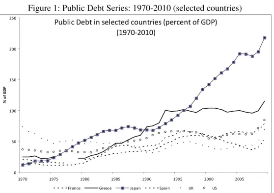
Figure 1: Public Debt Series: 1970-2010 (selected countries)

Public Debt in selected countries (percent of GDP) (1970-2010)

0 50 100 150 200 250

1970 1975 1980 1985 1990 1995 2000 2005

%

o

f

G

D

P

France Greece Japan Spain UK US

Source: Abbas et al. (2010).

For instance, government debt increased in Italy from an average of 51.8% of GDP in the 1970s to an average of 112.3% in the 2000s. In the case of Greece, Italy and Japan government debt has surpassed 100% of GDP, an average value that was kept during the 2000s. In the cases of Belgium and Italy, their high debt service payments induced substantial budget deficits despite primary surpluses. A reversal of that general trend is noticeable only at the end of the 1990s, as several “more indebted” European countries tried to fulfil or at least come closer to the Maastricht criteria (much of that effort was reversed in the most recent crisis). All in all, the main conclusion is that the burden of government debt has increased over time in almost every country under scrutiny.

Figure 2: Total Government Expenditures and Revenues: 1970-2010 (selected countries)

Government Expenditures in selected countries (percent of GDP)

(1970-2010)

15 35 55 75

1970 1975 1980 1985 1990 1995 2000 2005 2010

%

o

f

G

D

P

France Greece Japan Spain UK US

Government Revenues in selected countries (percent of GDP)

(1970-2010)

15 35 55 75

1970 1975 1980 1985 1990 1995 2000 2005 2010

%

o

f

G

D

P

France Greece Japan Spain UK US

Source: authors’ computations

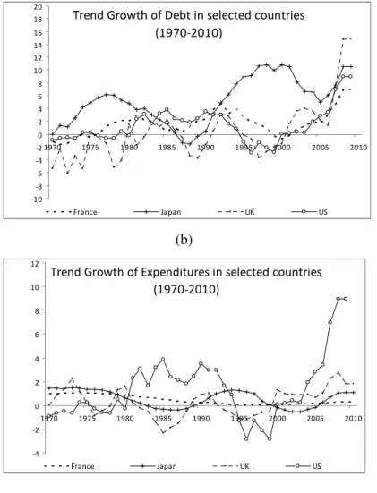
We continue with some descriptive statistics and in order to evaluate the possibility of the presence of a cyclical component in the series, objects such as the correlogram and the power spectrum can provide useful information. If sometimes the correlogram shows only small individual autocorrelations not providing enough strong evidence of the presence of cyclical movement in the series (despite some cycle evidence may be buried with noise), then a much clearer message emerges from the examination of the spectrum (not shown). Figure 3 shows the extracted (Structural Time Series Model-based)15 annual trend growth for total government debt, total government expenditures and total government revenues (all in % GDP), respectively in panels (a), (b) and (c) for France, Japan, the UK and the US (for reasons of parsimony).16

_____________________________

15 _{See Harvey (1989, 1991) for details. This class of models is preferred to other trend-cycle filters, as the HP. This}

one, which has been employed widely in the recent RBC literature, is not considered appropriate as it explicitly neglets low frequency swings by assumption and Harvey and Jaeger (1993) show that the HP filter may create spurious cycles and other distortions.

16 _{Upon careful examination of several descriptive statistics, a likely specification for the trend and the cycle has}

A few facts are worth noticing. Looking at Figure 3 a) we see that following Japan’s crisis in the early 1990s we observe a rise in the country’s debt trend growth till around 2000. It then decreased slightly until regaining impetus following the latest 2007-08 economic and financial crisis. For France, UK and US the biggest jump in the debt trend growth took place after the latest 2007-08 crisis. In panel b) the highest expenditures trend growth is attributed to the US which has been rising since the early 2000s and the events following the 9/11 of 2001 and wars against terror. Finally, the latest crisis has naturally affected the inflows of government revenues (panel c) ) with the most dramatic falls taking place once again in the US following the 9/11 and the latest crisis.

Figure 3: Trend Growth of Debt, Expenditures and Revenues, 1970-2010

(a)

Trend Growth of Debt in selected countries (1970-2010)

-10 -8 -6 -4 -2 0 2 4 6 8 10 12 14 16 18 20

1970 1975 1980 1985 1990 1995 2000 2005 2010

France Japan UK US

(b)

Trend Growth of Expenditures in selected countries (1970-2010)

-4 -2 0 2 4 6 8 10 12

1970 1975 1980 1985 1990 1995 2000 2005 2010

France Japan UK US

the hyperparameters for different structural time series models are available upon request. All these models assumed the presence of a trend, one cycle and an irregular component. Three STMs were considered: the first statistical specification assumed that the trend component follows a random walk with drift, with a deterministic

slope; the second introduced a somewhat smoother trend with adeterministic level and a stochastic slope; finally,

(c)

Trend Growth of Revenues in selected countries (1970-2010)

-2 0 2

1970 1975 1980 1985 1990 1995 2000 2005 2010

France Japan UK US

Source: authors’ computations

4.2 Country Analysis

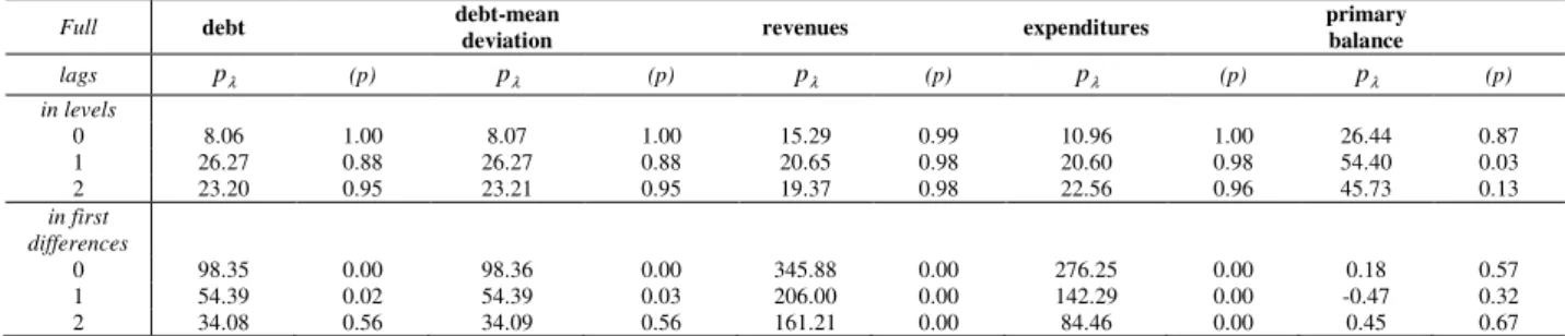
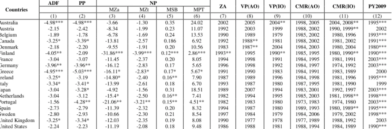
The fact that our series are in ratio to GDP does not rule them out being integrated processes (see, Ahmed and Yoo, 1989). Hence, we now focus on fiscal policy sustainability for each of the 18 countries by means of several unit root tests in an attempt to validate the sufficient sustainability condition using the stock of government debt. Table 1.a shows the stationarity tests results for the first difference of the debt ratio for the period 1970-2010.

The results for the ADF and PP test (considering both a constant and a time trend) allow the rejection of the null of a unit root only in Australia, Germany, Greece and the UK. Therefore the series of the first difference of government debt might be I(0) and the solvency condition would be satisfied in those cases since non-stationarity can be rejected. The Ng and Perron (2001) tests add Finland, Netherlands and Portugal to the “rejection-of-the-null” set of countries.17

[Table 1.a]

The previous set of results assumes that there is no structural break in the government debt series. However, this might not be the case in some countries – for example, in periods of war or important economic downturns. In the presence of structural changes in the trend function, ADF and PP tests that do not take into account the break in the series have low power, and are biased toward the non-rejection of a unit root. Therefore, in Table 1.a we also report the identified structural breaks. Depending on the precise test, we may get different results for break dates, with the overwhelmingly conclusion that most series are I(1), apart from Australia, Canada, Denmark and Finland for the ZA, VP and CMR tests. For instance, we get reported breaks for Finland in 1990-1993, time when the country was experiencing a severe recession.For Portugal _____________________________

17 _{One should also note that the number of observations used is only 41 at most, and the accuracy problems of}

unit-root tests with small samples are well known. Afonso and Jalles (2011) make use of the longer time series debt data

we get dates around 1974, 1982-83 and 2003, corresponding to the “Carnation Revolution”, the IMF program intervention and one severe recession, respectively.18 One can also note the different power attributed to the PY2009 test (particularly as the ZA and VP tests are conservative in the I(0) case, and have lack of power in the I(1) case) where in all but 4 cases we reject the null of unit root.

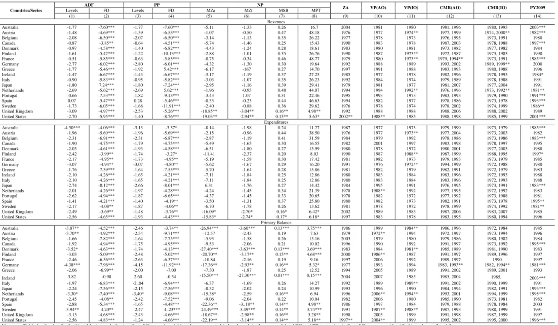
Turning to total government expenditures, total government revenues and the primary balance series (all in % GDP) - Table 1.b - we find similar results, with the non-rejection of the null of unit root in levels for most countries (apart from Australia in the case of expenditures and primary balance, and Germany and Sweden in the case of the primary balance). We observe fewer rejections of the null of unit root in the break-type tests (in particular, Austria, Finland, France and the Netherlands for the VP test in the revenues’ case; Austria, Finland and Germany for the VP test in the expenditures’ case; and Australia, Austria. Denmark Finland, Netherlands, Sweden and the US for the ZA and VP tests in primary balance case).

[Table 1.b]

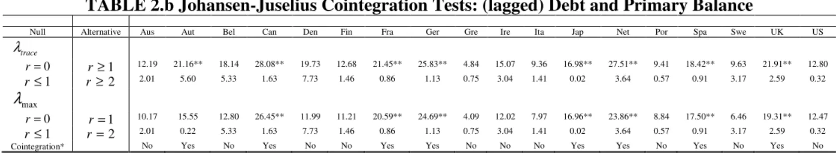
Stationarity aside, we now address the cointegration issue, given by (10) and (11), by analysing the relationship between revenues and expenditures and between the primary balance and (lagged) debt. Table 2.a presents the results for the Johansen-Juselius cointegration test for the former case. We find evidence of one cointegrating relationship in only 6 countries (Australia, Austria, Denmark, Germany, Japan and Netherlands); whereas in Table 2.b (for the latter case), we find evidence of cointegration in 8 countries (Austria, Canada, France, Germany, Japan, Netherlands, Sweden and the UK). Therefore, one would not reject the idea that public finances have been less unsustainable in those countries. Moreover, in these cases results from the Hansen-stability test did not reject the null hypothesis that the series are cointegrated at conventional levels (with p-values larger than 20%). Overall, test results allow the rejection of the cointegration hypothesis for the majority of the countries in both relationships under scrutiny.

[Table 2.a, 2.b]

As previously discussed in Section 3.1.1 we further test the hypothesis of a structural shift in the cointegration relationship for all countries in our sample, by using the Gregory and Hansen (1996) procedure. Table 3 presents our results. After taking into account the possibility of breaks in the series, we get for the revenues-expenditure relationship, rejections of the null of no

_____________________________

cointegration in 9 countries for the ADF* statistic (relatively in line with previous findings);19 similarly for the balance-(lagged) debt relationship, we reject the null in only 4 countries. In other words, for the period 1970-2010, government expenditures, in half of the countries, exhibited a higher growth rate than public revenues, challenging therefore the hypothesis of fiscal policy sustainability.

[Table 3]

We are now in position to estimate the parameter β (10) and (11). The estimation is made

using the DOLS of Stock and Watson (1993) as previously described. The results of the estimation of this equation for each country, in terms of the coefficient β and the statistic C_µ, a

LM statistic from the DOLS residuals, which tests for deterministic cointegration (i.e., when no trend is present in the regression), appear in Table 4. Two main results can be obtained from Table 4.a. First, since most of the cointegration statistics are highly significant at usual levels, the null of deterministic cointegration is rejected (less so in the case of the (lagged) debt-primary balance relationship). And, second, the estimates of β are in 15 out of 18 cases positive and

statistically significant for the revenues-expenditures relationship. Moreover, they are always less than one, that is, for each percentage point of GDP increase in public expenditures, for instance in Denmark and in Canada, public revenues only increase by respectively 0.70 and 0.33 percentage points of GDP. In the case of the primary balance-debt relationship we obtain positive and statistically significant estimates of β in 8 out of 18 cases (our results are in line

with Bajo-Rubio et al. (2009) findings).

[Table 4.a]

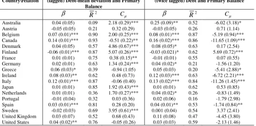
As two robustness checks, we have redone the exercise by: i) allowing for more lags in (10), that is, this time testing cointegration between the primary balance and the second lagged debt ratio; and ii) testing cointegration between the primary balance and the lagged debt deviation to each country’s mean over the entire period. Results (see Table 4.b) yield positive and statistically significant estimates of β in 9 (7) out of 18 cases for the former (latter) exercise

and roughly corresponding to the same set of countries.20 Therefore, the conclusion that emerges is that we cannot say that fiscal policy has been sustainable for half of the countries in our sample.

_____________________________

19 _{Our results, as most of the results reported in the literature, were obtained without considering additional sources}

of government revenues: for instance, seignorage and privatization revenues. Additionally, government assets

(wealth) should be taken into account to make judgements about the sustainability of public finances (even though data are mostly lacking).

20 _{We thank an anonymous referee for helping us explore additional possible channels through which cointegration}

[Table 4.b]

An additional exercise is to explore the causality direction between total government revenues and expenditures. Table 5.a present our results for the standard Granger causality test but also the Toda-Yamamoto one. In general, focusing on the former test first, evidence suggests stronger effects running from revenues to expenditures. In Canada, however, two-way causality is found, that is, we have “fiscal synchronization” in line with the assumption of equivalency between the marginal costs and marginal revenues that the utility-maximization suppliers and demanders of the public services make. It seems that in only 6 cases we have causality running from expenditures to revenues (the “spend and tax” hypothesis), meaning that the majority of fiscal authorities are not able to generate the revenues required to finance the planned expenditures; that is, the authorities have not kept fiscal budgets under control. Similar conclusions result from inspecting the Toda-Yamamoto test with Germany and Netherlands emerging as the two cases where two-way causality is present, that is, where we have “fiscal synchronization”.

[Table 5a]

As remarked before, in equilibrium the fiscal solvency condition holds in both the MD and FD regimes and the positive estimates of β found in Table 4 can be found in both of them.

Hence, Table 5.b presents the results from the standard Granger-causality tests together with the Toda-Yamamoto version, similarly to Table 5.a. Two-way causality was found in Italy in the former test, and in Japan and the Netherlands in the latter test. For these countries results from causality tests do not allow us to conclude whether fiscal solvency would have followed a MD or FD regime between 1970 and 2010. Granger-causality just from primary balance to debt appears for Finland, Ireland, Spain and the UK. On the other hand, Granger causality from government debt to the primary balance is found for 12 countries, which can be seen as evidence of the existence of a Ricardian regime.

[Table 5b]

4.3 Panel Analysis

are taken in levels.21 These results strongly indicate that the variables are non-stationary in level and stationary in first differences (with the exception of the primary balance with first generation panel unit root tests – Table B1, last column).

Table 6 shows the outcomes of Pedroni’s (1999) cointegration tests between total government revenues and expenditures and the primary balance and (lagged) debt. We use four within-group tests and three between-group tests to check whether the panel data are cointegrated. The columns labelled within-dimension contain the computed value of the statistics based on estimators that pool the autoregressive coefficient across different countries for the unit root tests on the estimated residuals. The columns labelled between-dimension report the computed value of the statistics based on estimators that average individually calculated coefficients for each country. Results of the within-group tests and the between-group tests show that the null hypothesis of no cointegration can be rejected. Therefore, the relationships identified in equations (10) and (11) are cointegrated for the panel of all countries in our sample.22

[Table 6]

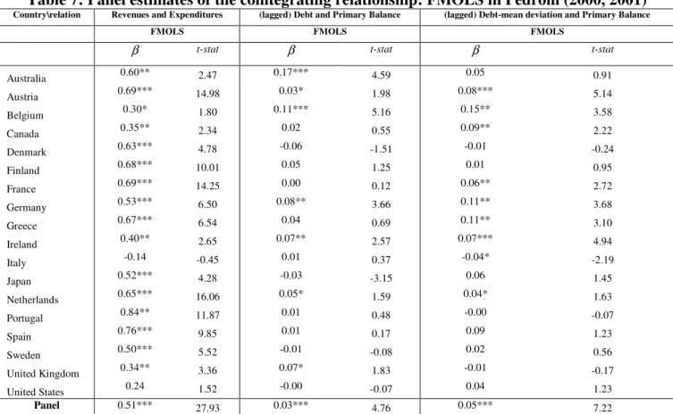
We then estimate the cointegrating vector using the FMOLS estimator. Table 7 shows the coefficients obtained with this estimator. The estimated coefficient for the pool of all countries is 0.51 and 0.03 (statistically significant at the 1% level) for the revenues-expenditures and primary balance-debt relationships, respectively. Focusing on the former, as before (Table 4), it seems that in general the greatest share of results point to a positive long-run co-movement between the levels of total government revenues and expenditures. On the second relationship, the average result points to solvency, even though, a country-by-country inspection shows that only Australia, Belgium, Germany, Ireland, Netherlands and the UK present statistically significant positive coefficient estimates for the improvement of the primary balance when there is a past worsening of the debt ratio. This result improves slightly if one considers the (lagged) debt-mean deviation variable instead. That is, a country-by-country inspection shows that now Austria, Belgium, Canada, France, Germany, Greece, Ireland, Italy and Netherlands present statistically significant positive coefficient estimates.

[Table 7]

_____________________________

21 _{Panel stationarity was also conducted for the debt deviation to the mean for each country in our dataset over the}

entire period. Results are in line with the ones for the original first difference debt variable (see Appendix B).

Turning to the Pedroni causality tests, one should note first that despite the fact that these tests can be implemented on a country-by-country basis23, in practice the reliability of these various point estimates and associated tests for any one country is likely to be poor given the relatively short time sample over which the data are observed. Therefore, our tests will be panel based. In particular, we want to know more about the pervasiveness of a long-run causal effect in the panel rather than simply finding that there is at least some long-run causality present in at least one specific country. To this end, we use both a group mean based test24 and a lambda-Pearson based test25. The combination of the group mean and the lambda-Pearson can be particularly informative when the underlying parameters of interest are heterogeneous. For

instance, when t_λ1fails to reject he null while

1

λ

P succeeds in rejecting the null, this can be

interpreted as a situation in which we do not reject that the average value for λ1iis zero, even

though we reject that it is pervasively zero in the panel.26 The results for each of these panel tests for the direction of long-run causality and the sign of the long-run causal effect are reported in Table 8.

[Table 8]

In examining the details of Table 8, panel A, the first note goes to the λ1iparameters as

reported in columns 2 through 4, which indicate that long-run causality that does not run from expenditures to revenues (p-values above 10%). This confirms our earlier “time-series” findings, that is, the non-validity of the “Spend and Tax” hypothesis, meaning that most fiscal authorities are not able to generate the revenues required to finance the planned expenditures. Turning

toλ2i, we reject the hypothesis that revenues have a zero average long-run effect globally (group

mean tests) on spending. The results hold pervasively among individual countries and on average for the entire panel (based on the group-mean and Lamba-Pearson tests). The

_____________________________

23 _{Results are available upon request.}

24 _{The group mean test is based on the sample average of the individual country}

i

1

λ tests and will allow us to ask

whether the long-run causal effect is zero on average for the panel. The group mean panel estimate is computed as

i i N

N 1 1 ₁

1

λ

λ

productivity is computed as

i t N

t Ni

1

1 1

1

λ

λ =

− Σ

= , where

i

t_λ1 is the individual country test for the null that λ_1i =0.

25 _{The lambda-Pearson panel test uses the p-values associated with each of the individual country}

t-tests to compute

the accumulated marginal significance associated with these. It takes the form

i p

P Ni

1

1 2 1ln λ

λ =− Σ = , where

i

p

1

ln _λ is the log of the p-value associated with individual country i’s t-test for the null that λ_1i =0.

26 _{This can occur when the value for}

i

1

λ is significantly positive for some fraction of the panel and significantly

implication of these results is that changes in revenues appear to induce permanent changes in long-run expenditures. On average the marginal long-run impact is zero.

Turning to Table 8, panel B, looking at the λ_1iparameters we conclude that long-run causality

seems to run from lagged debt to the primary balance (p-values below 10%). This confirms our previous “time-series” results, that is, we cannot reject that government debt Granger causes the primary balance. The results hold pervasively among individual countries and on average for the

entire panel (based on the group-mean and Lamba-Pearson tests). Turning toλ2i, we cannot

reject the hypothesis that primary balances have a zero average long-run effect globally (group mean tests). In other words, there is no long-run causality in this case running from the primary balance to government debt. At the same time, the sign of the effect is mixed, so that the average is still zero. As before, on average the marginal long-run impact is zero.

In order to control additionally for other effects on the a fiscal reaction specification as (10), we have made the estimation using information on financial crisis The rational is that when such crisis occur, the response of primary balances to increases in government indebtedness will tend to be lower, given the additional effort asked to public finances under those circumstances. Therefore, we use financial crises dummies derived from Leaven and Valencia’s (2010) publicly available database, and use them both in an additive and multiplicative (with the debt variable) in a pooled estimation of (1).

[Table 9]

The results in Table 9 show that financial crisis negatively impinge on the primary balance, as expected, and this is a consistently statistically significant result. For instance, in the case of the multiplicative dummy, the overall reaction of the primary balance to government debt developments may even be reversed, undermining fiscal sustainability.27

5. Conclusion

In this paper we have revisited the issue of fiscal policy sustainability in a sample of 18 OECD countries, with annual data between 1970 and 2010, by means of both time-series and panel data techniques. Our main results point to the non-stationarity of the first-differenced debt series for most countries (with the exception of Australia, Germany, Greece and the UK with the ADF and PP tests and adding Finland, Netherlands and Portugal with the Ng and Perron tests) suggesting that the solvency condition would not be satisfied. We find similar results in the

_____________________________

27_{For instance, in column (3) in Table 9, we have: / 0.014 0.049}

s B FC

∂ ∂ = − , implying an effect of -0-035 when a

cases of total government expenditures, total government revenues and the primary balance series, with the non-rejection of the null of unit root (in levels) for most countries.

Moreover, evidence suggests the existence of one cointegrating relationship in only 6 countries between revenues and expenditures. However, the overall test results allow the rejection of the cointegration hypothesis in both relationships under scrutiny. In other words, for the period 1970-2010, government expenditures, in half of the countries, exhibited a higher growth rate than public revenues, challenging therefore the hypothesis of fiscal policy sustainability.

Estimating the cointegrating coefficient we get 15 out of 18 cases positive and statistically significant estimates for the revenues-expenditures relationship and these are always less than one, that is, for each percentage point of GDP increase in public expenditures, revenues increase by less than one percentage point of GDP.

In terms of individual-country causality, evidence suggests stronger effects running from revenues to expenditures. Moreover in only 6 cases we have causality running from expenditures to revenues (the “spend and tax” hypothesis), meaning that the majority of fiscal authorities are not able to generate the revenues required to finance the planned expenditures. On the other hand, Granger causality from government debt to the primary balance is found for 12 countries, which can be seen as evidence of the existence of a Ricardian regime.

Our panel data results corroborate time-series findings with the greatest share of empirical evidence pointing to a positive long-run co-movement between the levels of total government revenues and expenditures, that is, changes in revenues appear to induce permanent changes in long-run expenditures.

Even tough we find that long-run causality seems to run from lagged debt to the primary balance, on average the marginal long-run impact is zero. All in all, we cannot say that fiscal policy has been sustainable for many countries in our sample.

References

1. Afonso, A. (2005), “Fiscal Sustainability: the Unpleasant European Case”, FinanzArchiv, 61 (1), 19-44.

2. Afonso, A. (2008), “Ricardian Fiscal Regimes in the European Union”, Empirica, 35 (3), 313–334. 3. Afonso, A. (2010), “Expansionary fiscal consolidations in Europe: new evidence”, Applied

Economics Letters, 17(2), 105-109.

5. Afonso, A., Jalles, J. (2011). “A longer-run perspective on fiscal sustainability”, ISEG-UTL, Department of Economics, Working Paper nº 17/2011/DE/UECE.

6. Afonso, A, Jalles, J. (2011). “Appraising fiscal reaction functions”, Economics Bulletin, 31 (4), 3320-3330.

7. Ahmed, S. and Rogers J. H. (1995), “Government budget deficits and trade deficits Are present value constraints satisfied in long-term data”, Journal of Monetary Economics 36(2), 351-374.

8. Ahmed, S. and Yoo, B. (1989), “Fiscal trends and real business cycles”, Working paper, Pennsylvania State University, University Park, PA.

9. Andrews, D.W. K., and Ploberger, W. (1994), “Optimal Tests When a Nuisance Parameter Is Present Only Under the Alternative”, Econometrica, 62, 1383-1414.

10. Arellano, M. and Bover, O. (1995), "Another Look at the Instrumental Variable Estimation of Error Component Models", Journal of Econometrics, 68: 29-51.

11. Arghyrou, Michael G. and Kul B. Luintel (2007), “Government Solvency: Revisiting Some EMU Countries”, Journal of Macroeconomics 29, 387-410.

12. Bajo-Rubio, Óscar, Díaz-Roldán, Carmen and Esteve, Vicente (2009), “Deficit sustainability and inflation in EMU: An analysis from the Fiscal Theory of the Price Level”, European Journal of Political Economy, 25(4), 525-539.

13. Barro, R., (1979), “On the Determination of the Public Debt,” Journal of Political Economy, 87, 940-971.

14. Bergman, M. (2001), “Testing Government Solvency and the No Ponzi Game Condition”, Applied Economics Letters, 8(1), 27-29.

15. Blanchard, O., J.C. Chouraqui, R.P. Hagemann and N. Sartor (1990), “The sustainability of Fiscal Policy: New Answers to an Old question”, OECD Economic Studies, 15, 7-36.

16. Bohn, H. (1991), “The Sustainability of Budget Deficits with Lump-Sum and with Income-Based Taxation”, Journal of Money, Credit, and Banking 23 (3), Part 2: 581-604.

17. Bohn, H. (1998), “The Behavior of U.S. Public Debt and Deficits”, Quarterly Journal of Economics 113, 949-963.

18. Bohn, H. (2007), “Are Stationarity and Cointegration Restrictions Really Necessary for the Intertemporal Budget Constraint?” Journal of Monetary Economics, 54(7), 1837-1847.

19. Bravo, A. B. S., Silvestre, A. L. (2002), “Intertemporal Sustainability of Fiscal Policies: Some Tests for European Countries”, European Journal of Political Economy, 18, 517–528.

20. Bruggeman, A., P. Donati, and A. Warne (2003), “Is the Demand for Euro Area M3 Stable?”, European Central Bank - Working Paper Series, No. 255.

21. Canning, C. and Pedroni, P. (2008), “Infrastructure, Long Run Economic Growth and Causality Tests for Cointegrated Panels”, Manchester School, 76, 504-527.