Fiscal Sustainability: the Unpleasant European Case

(1)

Fiscal Sustainability: the Unpleasant European Case

*

António Afonso

**

June 2004

Abstract

The sustainability of fiscal deficits has been receiving increasing attention. The issue is paramount for the newly formed euro area and this is one of the motivations of this paper. In order to assess the sustainability of budget deficits, co-integration tests between public expenditures and public revenues, allowing for structural breaks, are performed for the EU countries for the 1970-2003 period. The “unpleasant” empirical results show that with few exceptions fiscal policy may not have been sustainable. EU governments therefore could risk becoming inherently highly indebted, even if the debt-to-GDP ratios seemed to be somehow stabilising at the end of the 1990s. (JEL: H62, H63)

Keywords: Deficit finance; intertemporal budget constraint; fiscal policy sustainability; European Union

*

The author is grateful to Jorge Santos, João Santos Silva, and participants at conferences and seminars held in Lisbon, and Athens, for helpful comments. Any remaining errors are the responsibility of the author. The opinions expressed herein are those of the author and do not necessarily reflect those of the author’s employer.

**

European Central Bank, Kaiserstraße 29, D-60311 Frankfurt am Main, Germany, email: antonio.afonso@ecb.int.

(2)

1. Introduction

In the last two decades several developed countries have experienced significant budget

deficits, while the ability of government to cope with fiscal deficits has been receiving

increasing attention from economists. This is an important topic both in terms of

economics and public policy. The issue is paramount for the newly formed euro area and

this is one of the motivations of this paper. Theoretically, equilibrium growth paths need

to be supported by adequate fiscal policy.

Furthermore, the Treaties governing the European Union impose the practical necessity

of sustainable public accounts. It is possible to assess sustainable public finances in terms

of compliance with the budgetary requirements of the European Monetary Union, i.e.

avoiding excessive deficits, keeping debt levels below the 60 percent of GDP reference

value, and respecting the “close to balance or in surplus” requirement of the Stability and

Growth Pact (SGP). From a forward-looking perspective, one may also notice that the

SGP imposes commitments on Member States for budgetary positions in the

medium-term (three to five years) and does not require explicit longer-medium-term targets. Therefore,

sustainability is de facto ensured provided budget balances respect the “close to balance

or in surplus” target.

Quite a few studies have already addressed the issue of fiscal policy sustainability and

provided empirical testing of the Present Value Borrowing Constraint (PVBC)1. The

main analytical apparatus used to analyse the sustainability of budget deficits are

stationarity tests for the stock of public debt and co-integration tests between government

expenditures and government revenues. This paper adds to the existing literature by

applying unit root and co-integration tests to the EU-15 countries over the period

1970-2003, using consistent public finance data from one single source, the European

Commission AMECO database. It also tests for the existence of structural breaks during

the time sample in each country. The selected time span includes therefore the run up to

1

(3)

the introduction of the euro and the efforts, made during the 1990s, by several countries

to streamline their public accounts in order to join the common currency. Additionally,

both the theoretical and analytical procedures used to assess fiscal sustainability are

briefly restated.

The paper is organised as follows. The next section discusses the issue of sustainability.

Section three briefly reviews the analytical framework under which one usually assesses

the sustainability of public deficits. Section four presents some stylised facts of fiscal

policy for the EU countries. It also reports and discusses the results of the empirical

analysis, comprising both stationarity tests and co-integration tests between government

expenditures and government revenues for the EU-15 countries, allowing for structural

breaks in the series or in the co-integration relationship. Finally, section five provides a

conclusion.

2. The issue of sustainability

Fiscal sustainability seems a recurrent topic that both individual countries and

international organisations dwell upon with some regularity2. At the beginning of the

1920s, when writing about the public debt problem faced by France, Keynes (1923, p. 24)

mentioned the need for the French government to conduct a sustainable fiscal policy in

order to satisfy its budget constraint. Keynes stated that the absence of sustainability

would be evident when “the State's contractual liabilities (…) have reached an excessive

proportion of the national income.” In modern terms, sustainability is challenged when

the debt-to-GDP ratio reaches an excessive value. There is a problem of sustainability

when the government revenues are not enough to keep on financing the costs associated

with the new issuance of public debt.

The sustainability of fiscal policy is sometimes associated with the financial solvency of

the government. In practice however, what the empirical literature ends up testing is

whether both public expenditures and government revenues may continue to display in

the future their historical growth patterns. If a given fiscal policy turns out to be

2

(4)

unsustainable, it has to change in order to guarantee that the future primary balances are

consistent with the budget constraint3. Theoretically any value for the budget deficit

would be possible if the government could raise its liabilities without limit. Obviously,

that is impossible since the government is faced with the present value of its own budget

constraint.

It also is worthwhile noticing that the hypothesis of fiscal policy sustainability is related

to the condition that the trajectory of the main macroeconomic variables is not affected

by the choice between the issuance of public debt or the increase in taxation. Under such

conditions, it would therefore be irrelevant how the deficits are financed, implying also

the assumption of the Ricardian Equivalence hypothesis.

The government budget constraint is the starting point to derive the present value of the

budget constraint. The flow budget constraint is written as

t t t t

t r B R B

G +(1+ ) _-1 = + , (1)

where G is the government expenditures, excluding interest payments, R is the government revenues, B is the public debt and r is the real interest rate4. Rewriting equation (1) for the subsequent periods, and recursively solving that equation leads to the

following intertemporal budget constraint:

å

Õ

¥ = = + + = + + + + ¥ ® + + -= 1 1 1 ) 1 ( lim ) 1 ( s s

j t j

s t s j j t s t s t t r B s r G R

B . (2)

3

Cuddington (1997) and Hénin (1997) discuss this topic. Blanchard et al. (1990) present as a definition of sustainable fiscal policy one that allows, in the short-term, that the debt-to-GDP ratio returns to its original level after some excessive variation.

4

(5)

When the second term from the right-hand side of equation (2) is zero, the present value

of the existing stock of public debt will be identical to the present value of future primary

surpluses. However, equation (2) is not appropriate for empirical testing. It is therefore

useful to make several algebraic modifications to equation (1). Assuming that the real

interest rate is stationary, with mean r, and defining

1 ) ( -+

= t t t

t G r r B

E , (3)

it is possible to obtain the following so-called PVBC:

å

¥ = + + + + + -+ ¥ ® + -+ = 0 1 1 1 ) 1 ( lim ) ( ) 1 ( 1 s s s t s t s t s t r B s E R r

B . (4)

A sustainable fiscal policy should ensure that the present value of the stock of public

debt, the second term of the right hand side of (4), goes to zero in infinity, constraining

the debt to grow no faster than the real interest rate. In other words, it implies imposing

the absence of Ponzi games and the fulfilment of the intertemporal budget constraint.

Faced with this transversality condition, the government will have to achieve future

primary surpluses whose present value adds up to the current value of the stock of public

debt. Put another way, public debt in real terms cannot increase indefinitely at a growth

rate beyond the real interest rate5.

It is also possible to derive the solvency condition, with all the variables defined as a

percentage of GDP6. The PVBC, with the variables expressed as ratios of GDP, with y being the GDP real growth rate, and neglecting for presentation purposes seigniorage

revenues, is then written as

5

See Joines (1991). McCallum (1984) discusses if this is a necessary condition to obtain an optimal growth trajectory for the stock of public debt.

6

(6)

t t t t t t t t t t Y R Y G Y B y r Y B -+ + + = -1 1 ) 1 ( ) 1 ( . (5)

Assuming the real interest rate to be stationary, with mean r, and considering also constant real growth, the budget constraint is then given by

[

]

) 1 ( 0 ) 1 ( 1 1 1 lim 1 1 + + + + ¥ = +

- ÷_ø

ö ç è æ + + ¥ ® + -÷ ø ö ç è æ + + =

_å

s s t s t s t s s t r y b s e r y

b r , (6)

with bt = Bt/Yt, et = Et/Yt and rt = Rt/Yt. When r > y, it is necessary to introduce a

solvency condition, given by 0

1 1

lim ( 1)

= ÷ ø ö ç è æ + + ¥ ® + + s s t r y b

s , in order to bound public debt

growth7. This yields the familiar result that fiscal policy will be sustainable if the present

value of the future stream of primary surpluses, as a percentage of GDP, matches the

“inherited” stock of government debt8.

3. Assessment of the sustainability of public deficits

A common practice in the literature, among the set of methods to evaluate fiscal policy

sustainability, is to investigate past fiscal data to see if government debt follows a

stationary process or to establish if there is co-integration between government revenues

and government expenditures9.

Recalling the PVBC, equation (4), it is possible to present analytically two

complementary definitions of sustainability that set the background for empirical testing:

i) The value of public current debt must be equal to the sum of future primary surpluses:

7

This implies that the growth rate of the debt-to-GDP ratio should be less than the factor

(

)

( 1)

) 1 /( ) 1 ( + + +y r s .

8

According to Buiter (2002), the intertemporal government budget constraint should be satisfied always and not only in equilibrium. This is Buiter's main criticism of the fiscal theory of price level.

9

(7)

å

¥ = + + + - -+ = 0 1

1 ( )

) 1 ( 1 s s t s t s

t R E

r

B ; (7)

ii) The present value of public debt must approach zero in infinity:

0 ) 1 ( lim 1 = + ¥ ® + + s s t r B

s . (8)

In order to test empirically the absence of Ponzi games, one can test the stationarity of the

first difference of the stock of public debt, using unit root tests developed by Dickey and

Fuller (1981) and by Phillips and Perron (1988).

It is also possible to assess fiscal policy sustainability through co-integration tests. The

implicit hypothesis concerning the real interest rate, with mean r, is also stationarity. Using again the auxiliary variable ( ) ₁

-+

= t t t

t G r r B

E , and the additional definition

1 -+

= t t t

t G rB

GG , the intertemporal budget constraint may also be written as

1 0

1 ₍₁ ₎

lim ) ( ) 1 ( 1 + + ¥ = + + - _®_¥ ₊ + D -D + = -

å

s s t s s t s t s t t r B s E R r R

GG , (9)

and with the no-Ponzi game condition, GGt and Rt must be co-integrated variables of

order one for their first differences to be stationary.

Assuming that R and E are non-stationary variables, and that the first differences are stationary variables, this implies that the series R and E in levels are I (1). Then, for equation (9) to hold, its left-hand side will also have to be also stationary. If it is possible

to conclude that GG and R are integrated of order 1, these two variables should be co-integrated with co-integration vector (1, -1), for the left-hand side of equation (9) to be

(8)

Therefore the procedure to assess the sustainability of the intertemporal government

budget constraint involves testing the following co-integration regression:

t t

t a bGG u

R ₌ ₊ ₊ . If the null of no co-integration, the hypothesis that the two I (1)

variables are not co-integrated, is rejected (with a high-test statistic), this implies that one

should accept the alternative hypothesis of co-integration. For that result to hold true, the

series of the residual ut must be stationary, and should not display a unit root. Several

conclusions concerning the intertemporal budget constraint may then be established:

i) When there is no co-integration, the fiscal deficit is not sustainable,

ii) When there is co-integration with b=1, the deficit is sustainable,

iii) When there is co-integration, with b < 1, government expenditures grow faster than government revenues, and the deficit may not be sustainable10.

Hakkio and Rush (1991) also demonstrate that if GG and R are non-stationary variables in levels, the condition 0 < b < 1 is a sufficient condition for the budget constraint to be obeyed. However, when revenues and expenditures are expressed as a percentage of GDP

or in per capita terms, it is necessary to have b = 1 in order for the trajectory of the debt to GDP not to diverge in an infinite horizon11. The procedure to test the sustainability of

fiscal policy may be summarised, in a graphical sequential overview, by Figure 1.

[Insert Figure 1 about here]

Before proceeding it seems adequate to close the present section by summarising the

empirical findings of several previous studies, concerning the issue of sustainability.

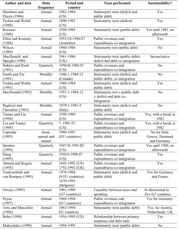
Therefore, Table 1 reviews the conclusions of those papers, which cover basically the US

and European countries, with sometimes quite conflicting results.

10

Concerning this co-integration analysis approach Bohn (1991, 1995) argues that a sustainable fiscal policy in a certain environment may become unsustainable under uncertainty.

11

(9)

[Insert Table 1 about here]

4. Fiscal policy sustainability in the EU-15 area

This section includes some stylised facts on fiscal policy during the 1970-2003 period for

the EU-15 countries. It also reports the unit root tests and estimation results of

co-integrating relations between expenditures and revenues.

4.1. Some stylised facts

A brief characterisation of the debt and fiscal burden for the EU countries is appropriate

before performing the empirical testing of the sustainability hypothesis. Between the

beginning of the 1970s and the end of the 1990s the debt-to-GDP ratio exhibited an

increasing trend for most countries throughout the period. For instance, general

government debt increased in Italy from 37.9 percent of GDP in 1970, to 110.6 percent of

GDP in 2000. In Germany the debt-to-GDP ratio was 18.2 percent in 1970 and went

beyond the 60 per cent level in 1997. According to European Commission data, in 2003

three countries still had a debt-to-GDP ratio above 100 percent (Italy, Belgium and

Greece), while in three other countries the debt ratio was higher than 60 percent (Austria,

Germany and France).

In the period 1970-2003 the highest debt-to-GDP ratios were reported in Italy and

Belgium (the country with the highest debt-to-GDP ratio in that period; reaching 138.2

percent in 1993), and their high debt service payments induced substantial budget deficits

despite primary budget surpluses. A reversal of that general trend is noticeable only at the

end of the 1990s, as the several “more indebted” countries tried to fulfil or at least come

closer to the Maastricht debt criterion.

The consequences of choosing different fiscal policies may be exemplified by looking for

instance at the public debt paths of some of the EU countries, as depicted in Figure 2. For

instance, the adding up of successive and significant budget deficits in Italy and in

(10)

ratio rising steadily until the middle of the 1990s. Germany and France also exhibited a

slowly growing debt ratio throughout the 1980s and 1990s. On the other hand, debt ratio

at the UK followed a downward path, while Ireland changed from being a high debt

country in the 1980s to a “less indebted” country in the 1990s.

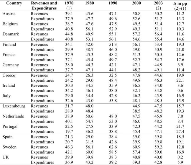
Concerning government expenditures and revenues, Table 2 reports those items as a

percentage of GDP for each country. The main conclusion is that the burden of public

expenditures and revenues on GDP has increased since the 1970s in almost every

country. Another obvious fact is that, , between 1970 and 2003, the ratio of government

expenditures to GDP, for most countries, exhibited a higher growth rate than the ratio of

government revenues to GDP. This conclusion holds for all countries except for Belgium,

Ireland and Italy. For instance in Italy, the ratios of government revenues and

expenditures to GDP were respectively 29 and 32.6 percent in 1970, compared with 45.9

and 48.5 percent in 2003.

4.2. Estimation results for the debt series

The focus of this sub-section and the next, is the study of fiscal policy sustainability for

each of the EU-15 countries. Augmented Dickey-Fuller (ADF) and Phillips-Perron (PP)

tests are used in an attempt to validate the sufficient sustainability condition, using the

stock of real public debt. Table 3 reports the stationarity tests results for the first

difference of the stock of public debt, at 1995 prices, for the period 1970-2003 (see data

sources in the Annex), considering both a constant and no trend.

The results allow the rejection of the null of a unit root for Austria, Portugal and the UK,

(11)

Portugal, Spain and Sweden, using the PP tests. Therefore the series of the first difference

of public debt might be I (0) for some countries, and the solvency condition would be

satisfied in those cases. However, if one considers also a time trend, then neither the ADF

nor the PP tests report that any of the series is I (0).

The previous results assume that there is no structural break in the debt series. However,

this might not be the case in some countries, namely for Germany due to reunification in

1990.12 In the presence of structural changes in the trend function, ADF and PP tests that

do not take account of the break in the series have low power and are biased toward the

non-rejection of a unit root. One procedure to test for unit roots in the presence of a

structural break involves splitting the sample into two parts and using the unit root tests

for each part. However, a resulting problem is that the degrees of freedom are diminished

for each of the parts.

Therefore, following Zivot and Andrews’ (1992) recursive approach, we tested the null

hypothesis that the series have a unit root against the alternative of stationarity with

structural change at some unknown break date denoted by TB.13 The break date is chosen

endogenously as the value, over all possible break points,14 which minimises the t -statistic for testing r=1 in the following regression:

t k

i

i t i t

B t

t t

t t Y DU DT D T c Y

Y = m+ b + r +q +g +d +

å

D +e =

-1

1 ( ) . (10)

The shift in the trend is given by DTt = t-TB, if t > TB, and 0 otherwise, and the shift in the

mean by DUt=1 if t > TB, and 0 otherwise. TB equals one at the observation after the

break point, while the additional one-time dummy D(TB)t=1 if t=TB+1 and 0 otherwise.

This “innovational outlier” model specifies that the change to the new trend function is

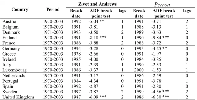
gradual. Table 4 reports the ADF test statistics proposed by both Zivot and Andrews

12

For instance, Greiner and Semmler (1999) report a break date for Germany in 1990, while Getzner et al. (2001) mention a break date in 1975 for Austria (but with a longer historical dataset).

13

This is a variation of the test of Perron (1988), with the advantage that the break point is estimated rather than fixed exogenously. See, for instance, Hansen (2001) for a review of these issues.

14

(12)

(1992) and by Perron (1994) for the best-fitted regression, alongside the estimated break

dates.15

The results allow for the rejection of the unit root hypothesis for Austria, Finland and the

UK, using the Zivot and Andrews test statistic, for Finland, Germany, Sweden and the

UK when the Perron test statistic is used. However, in general one cannot reject the

unit-root null at the 5 percent or 10 percent level, implying that there is not much evidence

against the unit-root hypothesis for most of the debt series in the EU-15 countries. These

results are, to some extent, in line with the standard unit-root tests reported previously in

Table 3.

Since some debt series might be stationary with breaks, the selected value of TB is a

consistent estimate of the break point. Interestingly, most of the reported breaks seem to

cluster in the 1990s, and more specifically in the first half of the decade, namely Austria

in 1991/92, Finland in 1990/91, and Germany in 1993/94. One can also notice that, for

instance, in Finland the debt-to-GDP ratio increased by more than threefold between

1990 and 1992 (while there was a severe recession in 1991/92). On the other hand, the

estimated break date for Germany occurs only in 1993.

One should also notice that the number of observations used is only 33 at most, and the

accuracy problems of unit root tests with small samples are well known. However, the

alternative approach of using quarterly data would constrain the time period, so that it is

therefore preferable to use a longer sample of annual data, instead of more observations

along a smaller time span. Furthermore, the rejection of the stationarity hypothesis does

not mean, as already noticed above, that public accounts are not sustainable, since as

Trehan and Walsh (1991) observe, the stationarity of the variation of the stock of public

debt is a sufficient condition, and stationarity rejection does not necessarily imply the

absence of sustainability in the government accounts.

15

(13)

4.3. Co-integration results

We now proceed to study fiscal sustainability in the EU-15 countries by testing the

existence of co-integration between government expenditures and revenues, taken as a

percentage of GDP, and using the sequential procedure depicted in Figure 1. Visual

inspection of the time series for each country may give an early clue, as can be seen by

the examples in Figure 3, which depict government expenditures and revenues, as a

percentage of GDP, for Italy, Germany, France and the Netherlands. One suspects in

advance that Italy and France may not pass the sustainability tests.

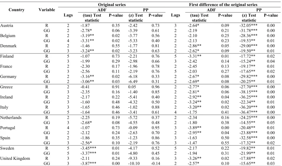
The first step is then to test the existence of a unit root for the government expenditures

and revenues as a percentage of GDP and to assess whether they are best characterised as

I(0) or as I(1) series. The results of those tests for the series in levels are presented in

Table 5.

It is possible to conclude that almost all series are not stationary in levels. There are some

exceptions where the ADF test statistic does not allow rejecting the hypothesis that the

series are I (0). However, this never happened with the PP test statistic, and allowing for a

trend in the regressions, both the ADF and the PP tests report that all series are

non-stationary. For every country it is thus necessary to test for the stationarity of the first

differences of the series.

According to the results also reported in Table 5, in general one would not reject the

stationarity of the first differences of the government expenditures and revenues series.

This is true for all series according to the PP test, but less generalised under the ADF test

statistics results. One can then tentatively assume that the first difference of the original

(14)

The Engle-Granger and Johansen co-integration tests were subsequently performed with

the government revenues and expenditures as a percentage of GDP. Co-integration tests

were made for all countries, even for the countries where the ADF test statistic (but not

the PP test) allows rejecting the null of unit root for the first difference of the revenue and

expenditure series. The co-integration results are presented in Table 6, but only for the

cases where there is a co-integrating vector with at least a significance level of ten

percent.

The test results allow the rejection of the co-integration hypothesis for the majority of the

countries, except for Austria, Germany, Finland, Netherlands, Portugal and the United

Kingdom. However, the estimated coefficients for expenditures, in the co-integration

equations, where government revenues are the dependent variable, are always less than

one. As a matter of fact, for each one percentage point of GDP increase in public

expenditures, for instance in the Netherlands and in Germany, public revenues only

increase respectively by 0.634 and 0.521 percentage points of GDP. Notice that these two

countries are the ones where the estimated coefficient b in the cointegrating vector (1, -b) has the highest absolute value. For the other countries where a significant

co-integration vector was found, b is even lower in absolute value.

In other words, for the period 1970-2003, government expenditures in the

abovementioned countries exhibited a higher growth rate than public revenues,

challenging therefore the hypothesis of fiscal policy sustainability. These results suggest

that fiscal policy may not have been sustainable for most countries with the possible

exceptions of Germany and the Netherlands.

However, and as in the case of unit roots, a test for co-integration that does not take into

account possible breaks in the long-run relationship will have lower power. The test will

tend to under-reject the null of no co-integration if there is a co-integration relationship

(15)

previous results, one should also entertain the possibility that the series are co-integrated

but that the linear combination has shifted at an unknown point in the data sample, in

other words, that there might be a relevant break date. Following Gregory and Hansen

(1996), the hypothesis of a structural shift in the co-integration relationships was then

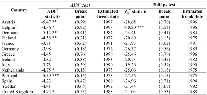
studied.16 Table 7 reports the results of the tests for regime shift (in level, with a time

trend) in co-integration of government revenues and expenditures for the EU-15

countries.

It is possible to see that for the above-mentioned countries, where a co-integration vector

was found, the test statistics from Table 7 broadly support the previous findings. Indeed,

accounting for the existence of break dates, the null of no co-integration is now rejected

for Austria, Belgium, Denmark, Finland, the Netherlands, Portugal and the UK, with the

ADF test statistic results (with the Phillips Za

*

test statistic the null is only rejected for

Belgium). This means that there is some long-run relationship in the data for those

countries. Notice also that the null of no co-integration is no longer rejected for Germany.

Additionally, the fact that the null hypothesis is now rejected for Belgium implies that

structural changes in the co-integration vector may be important. Since for the remainder

of the countries both ADF and ADF* test statistics reject the null of no co-integration, no

inference that structural change has occurred is warranted.

Our results, as most of the results reported in the literature were obtained without

considering additional sources of government revenues: for instance seigniorage and

privatisation revenues. Information on privatisation revenues is not easily available for

the EU-15 countries. Additionally, government assets (wealth) should be taken into

account to make judgements about the sustainability of public finances (even though data

are mostly lacking).

16

(16)

5. Conclusion

The fiscal policy sustainability issue has been reviewed and discussed in this paper, using

the government budget constraint as the key element of the analysis, and also the starting

point to derive analytical formulations suitable for empirical testing. Formally, the PVBC

requires that all future net tax revenues (i.e. tax revenues less transfers of current and all

future generations measured in present value terms) are enough to cover the present value

of future government consumption and to service the existing stock of government debt17.

The paper’s results reveal that with few exceptions, EU governments might have

sustainability problems, although debt-to-GDP ratios showed signs of stabilising at the

end of the 1990s. Using government expenditures and revenues as a percentage of GDP,

a co-integration approach was adopted. However, and even if a co-integration vector

were identified for Austria, Germany, Finland, Netherlands and Portugal, the estimated

coefficients for expenditures in the co-integration equations for those countries, where

public revenues is the dependent variable, are less than one.

The results of this paper are comparable with the ones from some of the existing

cross-country literature, and might be considered as “unpleasant” from a policy maker’s point

of view18. A small number of countries emerge as less likely to exhibit sustainability

problems, namely Germany, Netherlands, Finland, Austria the UK. Of these, Germany

and the Netherlands almost always appear as less likely to have sustainability problems.

However, our results also show that even for those two countries, the absolute value of

the relevant estimated coefficient in the co-integration relation is quite below unity

implying that their budget deficits may not be sustainable.

Therefore, the aforementioned countries face the problem of having a higher growth rate

for expenditures than the growth rate of revenues. In other words, if fiscal policy were to

be conducted in the future as it was in the past, there could still be some problems ahead,

17

One should note that it does not assume that government debt is ever paid off.

18

(17)

even for this set of countries that started, early in the 1990s, to make efforts in order to

meet strict budgetary criteria. This problem may even become more critical in the light of

some “unpleasant” available projections for the EU-15 countries, concerning future

public financial responsibilities. As a matter of fact, the EC (2001) reported that ageing

populations could lead to increased expenditure on public pensions by between 3 and 5

percentage points of GDP in most Member States, with larger increases in several

countries. Moreover, recent fiscal developments during 2001-2003 in several EU

countries do not seem reassuring in what terms of sustainability of public finances.

It is nevertheless important to keep in mind that the main driver for budgetary problems

in developed countries during future decades will be population growth combined with

generous pay-as-you-go financed social security systems. Since this population shift

towards older societies is an entirely new phenomenon, it cannot be considered in

econometric results based exclusively on past data. This does not constitute a general

criticism against purely econometric methods of measuring fiscal sustainability, but is

instead an argument for expanding the database. Indeed, implicit public pension

liabilities, as part of a country’s global fiscal imbalance, have to be understood as future

borrowing requirements, not fully embedded in the public fiscal figures, leading therefore

to added sustainability problems19. Also, one must recall that even for some of the

countries that are identified as not having had in the past an unsustainable policy, other

reports claim that sustainability may not be a feature of such countries’ fiscal policies20.

19

For a review of this topic and some interesting data simulation see, for instance, EPC (2003), Rother et al. (2003), and Holzmann et al. (2004).

20

(18)

Annex: Data sources

All data was taken from the European Commission AMECO (Annual Macro-Economic

Data) database, updated on 07/01/2004. The relevant AMECO codes are reported below.

- General government public debt (national currency). Code: UDGGL (linked series).

- Price deflator private of final consumption expenditure. Code: PCPH.

- General government total revenues, national currency. Code: URTG (ESA 1995);

URTGF (former definition).

- General government total expenditures, national currency. Code: UUTG (ESA 1995);

UUTGF (former definition).

- Gross domestic product, at market prices. Code: UVGDH (ESA 1995); UVGD (former

definition).

References

Ahmed, S. and Rogers, J. (1995). “Government budget deficits and trade deficits. Are present value constraints satisfied in long-term data?” Journal of Monetary Economics, 36 (2), 351-374.

Artis, M. and Marcelino, M. (1998). "Fiscal Solvency and Fiscal Forecasting in Europe," CEPR Discussion Paper 1836.

Baglioni, A. and Cherubini, U. (1993). “Intertemporal budget constraint and public debt sustainability: the case of Italy,” Applied Economics, 25 (2), 275-283.

Bergman, M. (2001). “Testing Government Solvency and the No Ponzi Game Condition,” Applied Economics Letters, 8 (1), 27-29.

Blanchard, O.; Chouraqui, J.; Hagemann, R. and Sartor, N. (1990). “The sustainability of fiscal policy: new answers to an old question,” OECD Economic Studies, 15, Autumn, 7-36.

Bohn, H. (1991). “The Sustainability of Budget Deficits with Lump-Sum and with Income-Based Taxation,” Journal of Money, Credit, and Banking, 23 (3), Part 2, 581-604.

(19)

Bohn, H. (1998). “The Behavior of U. S. Public Debt and Deficits, ” Quarterly Journal of Economics, 113 (3), 949-963.

Bravo, A. and Silvestre, A. (2002). “Intertemporal sustainability of fiscal policies: some tests for European countries,” European Journal of Political Economy, 18 (3), 517-528.

Buiter, W. (2002). “The Fiscal Theory of the Price Level: A Critique,” Economic Journal, 112 (481), 459-480.

Caporale, G. (1995). “Bubble finance and debt sustainability: a test of the government's intertemporal budget constraint,” Applied Economics, 27 (12), 1135-1143.

Chalk, N. and Hemming, R. (2000). “Assessing Fiscal Sustainability in Theory and Practice,” IMF Working Paper, 00/81, April.

Cuddington, J. (1997). “Analysing the Sustainability of Fiscal Deficits in Developing Countries,” Policy Research Working Paper nº 1784, World Bank.

Dickey, D. and Fuller, W. (1981). “The Likelihood Ratio Statistics for Autoregressive Time Series with a Unit Root,” Econometrica, 49, 1057-1072.

Elliot, G. and Kearney, C. (1988). "The intertemporal government budget constraint and tests for bubbles," Research Discussion Paper nº 8809, Reserve Bank of Australia.

EC (1999). “Generational accounting in Europe,” European Economy, Reports and Studies 6. Office for Official Publications of the EC.

EC (2001). “The impact of ageing populations on public pension systems,” European Economy, Reports and Studies 4. Office for Official Publications of the EC.

EPC (2003). “The impact of ageing populations on public finances: overview of analysis carried out at EU level and proposals for a future work programme,” Economic Policy Committee, EPC/ECFIN/435/03, October.

Fève, P. and Hénin, P. (2000). “Assessing effective sustainability of fiscal policy within the G-7,” Oxford Bulletin of Economic Research, 62 (2), 175-195.

Getzner, M.; Glatzer, E. and Neck, R (2001). “On the Sustainability of Austrian Budgetary Policies,” Empirica, 28 (1), 21-40.

Gregory, A. and Hansen, B. (1996). “Residual-based tests for cointegration in models with regime shifts,” Journal of Econometrics, 70 (1), 99-126.

(20)

Greiner, A.; Koeller, U. And Semmler (2004). “Debt Sustainability in the European Monetary Union: Theory and Empirical Evidence for Selected Countries,” mimeo.

Hakkio, G. and Rush, M. (1991). “Is the budget deficit "too large?"” Economic Inquiry, 29 (3), 429-445.

Hamilton, J. and Flavin, M. (1986). “On the Limitations of Government Borrowing: A Framework for Empirical Testing,” American Economic Review, 76 (4), 808-816.

Hansen, B. (2001). “The New Econometrics of Structural Change: Dating Breaks in U.S. Labor Productivity,” Journal of Economic Perspectives, 15 (4), 117-128.

Hatemi-J, A. (2002). "Fiscal Policy in Sweden: Effects of EMU Criteria Convergence," Economic Modelling, 19 (1) 121-136.

Haug, A. (1991). “Cointegration and Government Borrowing Constraints: Evidence for the United States,” Journal of Business & Economic Statistics, 9 (1), 97-101.

Haug, A. (1995). “Has Federal budget deficit policy changed in recent years?” Economic Inquiry, 33 (3), 104-118.

Hénin, P. (1997). “Soutenabilité des déficits et ajustements budgétaires,” Révue Économique, 48 (3), 371-395.

Holzmann, R.; Palacios, R. and Zviniene, A. (2004). “Implicit Pension Debt: Issues, Measurement and Scope in International Perspective,” Social Protection Discussion Paper No. 0403, March, World Bank.

Joines, D. (1991). “How large a federal deficit can we sustain?” Contemporary Policy Issues, 9 (3), 1-11.

Keynes, J. (1923). A Tract on Monetary Reform, in The Collected Writings of John Maynard Keynes, vol. IV, Macmillan, 1971.

Kremers, J. (1988). “The Long-Run Limits of U. S. Federal Debt,” Economics Letters, 28 (3), 259-262.

Kremers, J. (1989). “U. S. federal indebtedness and the conduct of fiscal policy,” Journal of Monetary Economics, 23 (2), 219-238.

Liu, P. and Tanner, E. (1995). “Intertemporal solvency and breaks in the US deficit process: a maximum-likelihood cointegration approach,” Applied Economics Letters, 2 (7), 231-235.

(21)

MacDonald, R. e Speight, A. (1990). “The intertemporal government budget constraint in the U.K., 1961-1986,” The Manchester School, 58 (4), 329-347.

Makrydakis, S.; Tzavalis, E. and Balfoussias, A. (1999). “Policy regime changes and long-run sustainability of fiscal policy: an application to Greece,” Economic Modelling, 16 (1), 71-86.

Martin, G. (2000). “US deficit sustainability: a new approach based on multiple endogenous breaks,” Journal of Applied Econometrics, 15 (1), 83-105.

McCallum, B. (1984). “Are Bond-Financed Deficits Inflationary? A Ricardian Analysis,” Journal of Political Economy, 92 (1), 123-135.

Olekalns, N. (2000). "Sustainability and Stability? Australian Fiscal Policy in the 20th Century," Australian Economic Papers, 39 (2), 138-151.

Owoye, O. (1995). “The causal relationship between taxes and expenditures in the G7 countries: cointegration and error-correction models,” Applied Economic Letters, 2 (1), 19-22.

Papadopoulos, A. and Sidiropoulos, M. (1999). "The Sustainability of Fiscal Policies in the European Union," International Advances in Economic Research, 5 (3), 289-307.

Payne, J. (1997). “International evidence on the sustainability of budget deficits,” Applied Economics Letters, 12 (4), 775-779.

Perron, P (1989). “The Great Crash, the Oil Price Shock, and the Unit Root Hypothesis,” Econometrica, 57 (6), 1361-1401.

Phillips, P. and Perron, P. (1988). “Testing for a Unit Root in Time Series Regression,” Biometrika, 75 (2), 335-346.

Perron, P. (1994). “Trend, Unit Root and Structural Change in Macroeconomic Time Series,” in Cointegration for the Applied Economist, Rao, B. (ed.), St. Martin’s Press.

Quintos, C. (1995). “Sustainability of the Deficit Process With Structural Shifts,” Journal of Business & Economic Statistics, 13 (4), 409-417.

Raffelhüschen, B. (1999). “Generational Accounting in Europe,” American Economic Review, Papers and Proceedings, 89 (2), 167–170.

Rother, P.; Catenaro, M; and Schwab, G. (2003). “Ageing and Pensions in the Euro Area Survey and Projection Results,” Social Protection Discussion Paper No. 0307, March, World Bank.

(22)

Tanner, E. and Liu, P. (1994). “Is the budget deficit "too large?": some further evidence,” Economic Inquiry, 32, 511-518.

Trehan, B. and Walsh, C. (1988). “Common trends, the government's budget constraint, and revenue smoothing,” Journal of Economic Dynamics and Control, 12 (2/3), 425-444.

Trehan, B. and Walsh, C. (1991). “Testing Intertemporal Budget Constraints: Theory and Applications to U.S. Federal Budget and Current Account Deficits,” Journal of Money, Credit, and Banking, 23 (2), 206-223.

Uctum, M. and Wickens, M. (2000). “Debt and deficit ceilings, and sustainability of fiscal policies: an intertemporal analysis,” Oxford Bulletin of Economic Research, 62 (2), 197-222.

Vanhorebeek, F. and van Rompuy, P. (1995). "Solvency and sustainability of fiscal policies in the EU," De Economist, 143 (4), 457-473.

Wilcox, D. (1989). “The Sustainability of Government Deficits: Implications of the Present-Value Borrowing Constraint,” Journal of Money, Credit, and Banking, 21 (3), 291-306.

(23)

Figure 1. Fiscal policy sustainability, unit root and co-integration tests

Unit root tests for R and GG

R is I (0) and GG is I (1); GG is I (1) and R is I (0)

There is no sustainability

R is I (0) and GG is I (0) Sustainability

R is I (1) and GG is I (1)

Co-integration tests between R and GG

R and GG are not co-integrated

There is no sustainability #

R and GG are co-integrated, CI (1,1)

Co-integrating vector (1, -b)

b = 1

Sustainability, with bounded debt-to-GDP ratio

b < 1

Sustainability, without bounded debt-to-GDP ratio

b > 1 There is no

sustainability

#

(24)

Figure 2. Public debt in some EU countries (percent of GDP)

0 20 40 60 80 100 120 140

1970 1972 1974 1976 1978 1980 1982 1984 1986 1988 1990 1992 1994 1996 1998 2000 2002

% of

G

D

P

BEL DEU FRA IRE ITA GBR

(25)

Figure 3. Government expenditures and revenues (percent of GDP)

3a. Italy 3b. Germany

25 30 35 40 45 50 55 60

1970 1973 1976 1979 1982 1985 1988 1991 1994 1997 2000 2003

% of

GDP

Revenues Expenditures

25 30 35 40 45 50 55 60

1970 1973 1976 1979 1982 1985 1988 1991 1994 1997 2000 2003

% of GDP

3c. France 3d. Netherlands

25 30 35 40 45 50 55 60

1970 1973 1976 1979 1982 1985 1988 1991 1994 1997 2000 2003

% o

f GD

P

25 30 35 40 45 50 55 60

1970 1973 1976 1979 1982 1985 1988 1991 1994 1997 2000 2003

% of GDP

(26)

Table 1. Some existing empirical evidence regarding fiscal policy sustainability

Author and date Data frequency

Period and country

Tests performed Sustainability?

Hamilton and Flavin (1986)

Annual 1962-1984 (US)

Stationarity tests (deficit and public debt)

Yes

Trehan and Walsh (1988)

Annual 1890-1983 (US)

Stationarity tests (deficit) Yes

Kremers (1988)

Annual 1920-1985 (US)

Stationarity tests (public debt) Yes until 1981, no afterwards Elliot and Kearney

(1988)

Annual 1953/54-1986/87 (Australia)

Public revenues and expenditures co-integration Yes Wilcox (1989) Annual 1960-1984 (US)

Stationarity test (public debt) No

MacDonald and Speight (1990)

Annual 1961-1986 (UK)

Stationarity tests (public debt); deficit and debt co-integration

Inconclusive

Hakkio and Rush (1991)

Quarterly 1950:II-1988:IV (US)

Public revenues and expenditures co-integration

No

Smith and Zin (1991)

Monthly 1946:1-1984:12 (Canada)

Stationarity tests (deficit and public debt), co-integration

No

Trehan and Walsh (1991)

Annual 1960-1984 (US)

Yes

MacDonald (1992) Monthly 1951:1-1984:12 (US)

Stationarity test s (public debt ); deficit and debt

co-integration No Baglioni and Cherubini (1993) Monthly 1979:1-1991:5 (Italy)

No

Tanner and Liu (1994)

Annual 1950-1989 (US)

Yes, with a break in 1982 Liu and Tanner

(1995)

Quarterly ? -1991:IV (US)

Yes, with a break in 1982 Caporale (1995) Semi-annual and annual 1960-1991 (EU countries)

No for Italy, Greece, Denmark and Germany Quintos (1995) Quarterly 1947:II-1992:III (US)

Yes until 1980, no afterwards Haug

(1995)

Quarterly 1950:I-1990:IV (US)

Yes

Ahmed and Rogers (1995)

Annual 1692-1992 (US) 1792-1992 (UK)

Yes

Vanhorebeek and van Rompuy (1995)

Annual 1970-1994 (8 EU countries) 1870-1993 (Belgium)

Yes for Germany and France

Owoye (1995) Annual 1961-1990 (G7 countries)

Causality between taxes and spending

bi-directional in five G7 countries Payne

(1997)

Annual 1949-1994 (G7 countries)

Yes for Germany

Artis and Marcelino (1998)

Annual 1963-1994 EU countries

Stationarity tests (public debt) Yes, for Austria, Netherlands, UK Bohn (1998) Annual 1916-1995 (US) Relationship between primary

surpluses and debt ratio

Yes

(27)

(Greece) Papadopoulos and

Sidiropoulos (1999)

Annual 1961-1995 (4 European countries)

Yes for Greece and Spain

Table 1. (continued)

Author and date Data frequency

Period and country

Tests performed Sustainability?

Greiner and Semmler (1999)

Annual 1955-1994 Germany

Stationarity tests (public debt) No

Olekalns (2000) Annual and quarterly 1900/01-1994/95 1978:3-1997:4 (Australia)

No

Fève and Hénin (2000)

Semi-annual

(G-7 countries) Stationarity tests (public debt) Yes for US, UK and Japan Uctum and

Wickens (2000)

Annual 1965-1994 (US and 11 EU countries)

Stationarity tests (public debt) Yes for Denmark, Netherlands, Ireland and France Martin

(2000)

Annual 1947-1992 (US)

Yes, with breaks in the 70s and 80s Getzner, Glatzer

and Neck (2001)

Austria 1960-1999 Stationarity tests (central public debt)

Yes for 1960-1974, no for 1975-1999 Bravo and Silvestre

(2002)

Annual 1970-1997 (EU countries)

Yes for Germany, Austria, Finland, UK, Netherlands Hatemi-J (2002) Quarterly 1963:I-2000:I (Sweden)

Public revenues and expenditures co-integration Yes Greiner, Koeller and Semmler (2004) Annual 1960-2003 (Germany, France, Italy, Portugal and US)

Relationship between primary surpluses and debt ratio

(28)

Table 2. General government revenues and expenditures, EU-15 (percent of GDP)

Country Revenues and Expenditures

1970

(1)

1980 1990 2000 2003

(2)

D in pp

(2)-(1)

Austria Revenues 39.1 45.6 47.1 50.8 50.2 11.2

Expenditures 37.9 47.2 49.6 52.6 51.2 13.3

Belgium Revenues 38.7 47.6 47.5 49.5 51.4 12.7

Expenditures 40.8 56.1 52.9 49.3 51.1 10.3

Denmark Revenues 44.8 49.9 55.1 57.2 56.4 11.6

Expenditures 40.8 53.1 56.1 54.6 55.4 14.6

Finland Revenues 34.1 42.0 51.3 56.1 53.4 19.3

Expenditures 29.9 38.7 46.0 49.0 50.9 21.0

France Revenues 37.9 45.3 48.2 51.3 50.5 12.6

Expenditures 37.1 45.4 49.7 52.7 54.7 17.6

Germany Revenues 38.0 44.3 42.1 47.1 44.9 6.9

Expenditures 37.7 47.1 44.1 48.2 49.1 11.4

Greece Revenues 24.7 26.3 32.5 47.8 44.6 19.9

Expenditures 24.2 29.0 48.4 49.8 46.3 22.1

Ireland Revenues 30.3 34.5 35.9 36.5 34.0 3.6

Expenditures 34.2 46.1 38.0 32.1 34.8 0.6

Italy Revenues 29.0 34.4 42.8 46.2 45.9 16.9

Expenditures 32.6 43.0 53.8 48.1 48.5 15.9

Luxembourg Revenues 31.7 48.0 44.9 47.5 15.7

Expenditures 28.9 48.4 38.5 48.2 19.3

Netherlands Revenues 38.9 50.6 48.0 47.5 45.9 7.0

Expenditures 40.1 54.7 53.0 46.0 48.5 8.4

Portugal Revenues 22.5 27.8 33.9 42.3 44.2 21.7

Expenditures 19.7 36.2 38.8 45.4 47.1 27.4

Spain Revenues 21.3 29.0 38.4 39.0 39.8 18.5

Expenditures 20.7 31.5 42.6 39.9 39.8 19.1

Sweden Revenues 46.3 56.1 62.6 60.9 59.2 12.8

Expenditures 42.1 60.0 58.5 57.4 59.0 16.9

UK Revenues 39.9 39.8 38.3 40.8 40.0 0.2

Expenditures 36.9 43.2 39.2 39.3 42.8 5.9

(29)

Table 3. Stationarity tests for the first difference of the stock of public debt, with constant, no trend (at 1995 prices)

ADF PP

Country Period lags (tau) Test statistic

P-value (z) Test statistic

P-value

Austria 1970-2003 3 -4.00 *** 0.00 -16.15 0.03

Belgium 1970-2003 5 -1.08 0.72 -4.05 0.53

Denmark 1971-2003 2 -2.26 0.19 -9.97 0.14

Finland 1970-2003 3 -2.41 0.14 -10.34 0.12

France 1977-2003 2 -2.50 0.12 -11.44 * 0.10

Germany 1970-2003 2 -2.50 0.13 -17.48 ** 0.02

Greece 1970-2003 2 -2.38 0.15 -26.89 *** 0.00

Ireland 1970-2003 5 -0.91 0.78 -18.35 ** 0.02

Italy 1970-2003 2 -1.20 0.67 -6.53 0.31

Luxembourg 1970-2003 2 -1.86 0.35 -13.45 * 0.06

Netherlands 1975-2003 2 -1.21 0.67 -7.71 0.24

Portugal 1973-2003 2 -3.77 *** 0.00 -29.11 *** 0.00

Spain 1970-2003 5 -2.02 0.28 -14.44 ** 0.05

Sweden 1970-2003 2 -2.50 0.12 -13.93 ** 0.05

United Kingdom 1970-2003 5 -3.13 * 0.10 -9.05 0.50

(30)

Table 4. Test for structural change in general government debt, (innovational outlier model)

Zivot and Andrews _Perron Country Period _Break

date

ADF break point test

lags Break date

ADF break point test

lags

Austria 1970-2003 1992 -5.04 ** 1 1991 -3.71 2

Belgium 1970-2003 1991 -3.81 1 1988 -3.13 1

Denmark 1971-2003 1993 -3.50 2 1989 -3.63 2

Finland 1970-2003 1991 -8.18 *** 1 1990 -9.84 *** 0

France 1977-2003 1988 -3.88 2 1988 -3.72 2

Germany 1970-2003 1994 -3.28 0 1993 -4.25 ** 0

Greece 1970-2003 1978 -2.66 0 1991 -1.97 0

Ireland 1970-2003 1985 -4.00 0 1984 -3.85 0

Italy 1970-2003 1991 -2.39 1 1990 -2.33 1

Luxembourg 1970-2003 1986 -3.37 1 2000 -1.53 1

Netherlands 1975-2003 1991 -3.17 0 1986 -2.59 0

Portugal 1973-2003 1984 -4.34 0 1991 -3.78 1

Spain 1970-2003 1992 -2.87 0 1991 -2.80 0

Sweden 1970-2003 1997 -3.87 2 1999 -4.56 *** 2

United Kingdom 1970-2003 1987 -6.09 *** 2 1986 -6.30 *** 2

(31)

Table 5. Stationary of government revenues and expenditures (percent of GDP), with constant, no trend

Original series First difference of the original series

ADF PP ADF PP

Country Variable

Lags (tau) Test statistic

P-value Lags (tau) Test statistic

P-value

Austria R 2 -1.87 0.35 -2.42 0.73 3 -2.64* 0.09 -32.05*** 0.00

GG 2 -2.78* 0.06 -3.39 0.61 2 -2.19 0.21 -31.78*** 0.00

Belgium R 2 -3.19** 0.02 -3.77 0.56 2 -2.10 0.25 -28.36*** 0.00

GG 4 -3.31** 0.02 -5.33 0.40 2 -2.13 0.23 -19.53** 0.01

Denmark R 2 -1.46 0.55 -1.77 0.81 2 -2.86** 0.05 -29.00*** 0.00

GG 3 -3.24** 0.02 -3.23 0.63 2 -2.62* 0.09 -19.50** 0.01

Finland R 5 -1.07 0.73 -2.21 0.76 5 -3.31** 0.01 -17.72** 0.02

GG 3 -1.99 0.29 -2.98 0.66 3 -2.42 0.14 -15.24** 0.04

France R 2 -2.30 0.17 -1.96 0.78 2 -2.45 0.13 -19.17** 0.01

GG 3 -2.56 0.11 -2.19 0.76 5 -2.03 0.27 -17.65** 0.02

Germany R 2 -3.16** 0.02 -6.18 0.33 2 -2.67* 0.08 -29.82*** 0.00

GG 2 -3.06** 0.03 -6.49 0.31 2 -2.69* 0.08 -20.25** 0.01

Greece R 2 -0.41 0.91 0.05 0.96 2 -2.77* 0.06 -27.70*** 0.00

GG 3 -2.35 0.16 -1.40 0.85 2 -2.81* 0.06 -38.15*** 0.00

Ireland R 2 -2.17 0.22 -5.41 0.40 2 -2.92** 0.04 -36.25*** 0.00

GG 3 -1.60 0.48 -4.32 0.50 2 -3.24** 0.02 -22.34** 0.01

Italy R 3 -1.65 0.46 -1.02 0.88 2 -3.20** 0.02 -36.20*** 0.00

GG 5 -1.64 0.46 -3.41 0.61 4 -1.75 0.41 -36.47*** 0.00

Netherlands R 2 -2.25 0.19 -5.72 0.37 2 -2.34 0.16 -24.25*** 0.00

GG 3 -2.68* 0.08 -4.55 0.48 2 -1.80 0.38 -14.55** 0.05

Portugal R 4 -1.07 0.73 -0.09 0.95 3 -3.89** 0.00 -20.48** 0.01

GG 2 -2.12 0.24 -2.63 0.70 2 -2.95** 0.04 -23.88*** 0.00

Spain R 2 -1.86 0.35 -1.23 0.86 3 -1.63 0.50 -32.58*** 0.00

GG 3 -2.56* 0.10 -2.19 0.76 3 -1.47 0.55 -17.32** 0.02

Sweden R 5 -3.45*** 0.01 -4.17 0.52 5 -2.17 0.22 -19.82** 0.01

GG 5 -3.37*** 0.01 -4.80 0.45 2 -1.94 0.31 -21.99** 0.01

United Kingdom R 3 -2.11 0.24 -9.33 0.16 3 -3.26** 0.02 -17.88** 0.02

GG 3 -3.87*** 0.00 -10.10 -0.14 2 -2.57* 0.10 -15.65** 0.03

(32)

Table 6. Co-integration of government revenues and expenditures (percent of GDP)

Engle-Granger (tau) co-integration test

Johansen (trace) co-integration test Country

Dependent variable

Vector P-valueAsy Vector P-valueAsy

R [1 -0.380]*** 0.008 [1 -0.418]** 0.035 Austria

GG [1 -1.609]* 0.084 [1 -2.395]**

R [1 -0.521]** 0.020 [1 -0.629]** 0.017 Germany

GG [1 -1.272]** 0.018 [1 -1.589]**

R [1 -0.343]** 0.022 [1 -0.368]* 0.070 Finland

GG - - [1 -2.719]*

R [1 -0.634]** 0.037 [1 -0.665]** 0.016 Netherlands

GG [1 -1.455]* 0.100 [1 -1.505]**

R [1 -0.205]*** 0.004 [1 -0.174]*** 0.009 Portugal

GG - - [1 -5.740]***

R - -

-United

Kingdom GG [1 –0.516]** 0.044 [1 -0.735]** 0.017

(33)

Table 7. Testing for regime shifts in co-integration of government revenues and expenditures (percent of GDP), level shift with time trend

ADF test Phillips test

Country _ADF*

statistic

Break point

Estimated break date

Za

*_statistic _Break

point

Estimated break date

Austria -5.47 ** (0.79) 1997 -28.65 (0.76) 1996

Belgium -4.86 * (0.82) 1998 -80.20 *** (0.53) 1996

Denmark -5.14 ** (0.41) 1984 -24.41 (0.41) 1984

Finland -4.58 ** (0.21) 1977 -20.89 (0.15) 1975

France -3.71 (0.62) 1991 -21.95 (0.62) 1991

Germany -3.98 (0.18) 1976 -26.37 (0.56) 1989

Greece -4.45 (0.76) 1996 -25.46 (0.76) 1996

Ireland -3.32 (0.38) 1983 -20.73 (0.35) 1982

Italy -3.73 (0.59) 1990 -19.26 (0.59) 1990

Netherlands -4.75 * (0.15) 1975 -25.06 (0.15) 1975

Portugal -5.59 *** (0.15) 1975 -27.56 (0.15) 1975

Spain -4.23 (0.47) 1986 -24.96 (0.71) 1994

Sweden -4.41 (0.65) 1992 -21.44 (0.65) 1992

United Kingdom -4.75 * (0.53) 1988 -21.05 (0.53) 1988

Notes: ADF* and Za

*

refer to the augmented Dickey-Fuller (ADF) and to the Phillips Za

*