3-SteP analySiS of Public financeS SuStainability the caSe of the euroPean union

WO R K I N G PA P E R S E R I E S

N O 9 0 8 / J U N E 2 0 0 8

3-STEP ANALYSIS OF

PUBLIC FINANCES

SUSTAINABILITY

THE CASE OF THE

EUROPEAN UNION

W O R K I N G PA P E R S E R I E S

N O 9 0 8 / J U N E 2 0 0 8

In 2008 all ECB publications feature a motif taken from the 10 banknote.

3-STEP ANALYSIS OF PUBLIC

FINANCES SUSTAINABILITY

THE CASE OF THE

EUROPEAN UNION

by António Afonso

and Christophe Rault

This paper can be downloaded without charge from http://www.ecb.europa.eu or from the Social Science Research Network electronic library at http://ssrn.com/abstract_id=1138608.

© European Central Bank, 2008

Address

Kaiserstrasse 29

60311 Frankfurt am Main, Germany

Postal address

Postfach 16 03 19

60066 Frankfurt am Main, Germany

Telephone

+49 69 1344 0

Website

http://www.ecb.europa.eu

Fax

+49 69 1344 6000

All rights reserved.

Any reproduction, publication and reprint in the form of a different publication, whether printed or produced electronically, in whole or in part, is permitted only with the explicit written authorisation of the ECB or the author(s).

The views expressed in this paper do not necessarily refl ect those of the European Central Bank.

Abstract 4 Non-technical summary 5

1 Introduction 7

2 Analytical framework for fi scal sustainability 9 3 Econometric strategy 11 3.1 Methodological issues 11 3.2 Series specifi c panel unit root test: SURADF 14 4 Investigating fi scal sustainability in the EU 16 4.1 Fiscal data 16 4.2 Step 1: unit root analysis 17 4.3 Step 2: panel cointegration 28 4.4 Step 3: SUR cointegration relationships 31

5 Conclusion 36

References 38

Annex: General government revenue

and expenditure 41 European Central Bank Working Paper Series 45

Abstract

We use a 3-step analysis to assess the sustainability of public finances in the EU27. Firstly, we perform the SURADF specific panel unit root test to investigate the mean-reverting behaviour of general government expenditure and revenue ratios. Secondly, we apply the bootstrap panel cointegration techniques that account for the time series and cross-sectional dependencies of the regression error. Thirdly, we check for a structural long-run equation between general government expenditures and revenues via SUR analysis. While results imply that public finances were not unsustainable for the EU panel, fiscal sustainability is an issue in most countries, with a below unit estimated coefficient of expenditure in the cointegration relation with revenue as the dependent variable.

Keywords: fiscal sustainability, EU, panel cointegration.

Non-technical summary

Studies on the sustainability of public finances regarding the European Union usually

restrict themselves to the set of EU Member States before the 1 May 2004 enlargement.

The choice of such group of countries is usually prompted by the lack of longer

comparable time series data for the new EU Member States. According to our

knowledge, this is the first fully fledged panel analysis of fiscal sustainability

encompassing the enlarged set of 27 EU countries. In this paper we assess the

sustainability of public finances, taking advantage of non-stationary panel data

econometric techniques and the Seemingly Unrelated Regression (SUR) methods,

covering several sub-periods within the period 1960-2006, and also defining different

country groupings for the several members of the EU.

More specifically, we use a 3-step analysis where we employ (i) SURADF panel

integration analysis, which seems to be the first empirical application in the context of

the sustainability of public finances; (ii) panel bootstrap to test the null hypothesis of

cointegration between expenditure and revenue ratios; (iii) SUR methods to assess the

magnitude of the estimated coefficient of revenues in the cointegration relationship.

The results of several panel unit root tests, notably the SURADF test, show that general

government revenue and expenditure-to-GDP ratios are not stationary for the

overwhelming majority of the EU27 countries. Additionally, at the conventional 5 and

10 per cent levels of significance, we can also conclude that a cointegration relationship

exists between government revenue and expenditure ratios for the EU14 panel data set

14 EU Member States before the 2004 enlargement, as well as the group including also

the more recent members of the EU, for the periods 1998-2006 and 2000-2006.

Moreover, for the countries where a cointegration relation exists, we then use the SUR

estimator, allowing for cross-country dependence among countries, to estimate the

coefficient of the expenditure ratio in a system were the revenue ratio is the independent

variable. However, and even if a cointegration vector was identified for all countries,

the estimated coefficient for expenditures, in the cointegration equations where public

revenues is the dependent variable, is usually less than one. In other words, for the

period 1960-2006, government expenditures in the EU14 (in the EU21 and EU22

countries for the more recent sub-periods) exhibited a higher growth rate than public

revenues, questioning the hypothesis of fiscal policy sustainability. These results

suggest that fiscal policy may not have been sustainable for most countries although it

may have been less unsustainable for such countries as Denmark, Finland, Luxembourg,

1. Introduction

Studies on the sustainability of public finances regarding the European Union usually

restrict themselves to the set of EU Member States before the 1 May 2004 enlargement.

The choice of such group of countries is usually prompted by the lack of longer

comparable time series data for the new EU Member States. According to our

knowledge, this is the first fully fledged panel analysis of fiscal sustainability

encompassing the enlarged set of 27 EU countries. In this paper we assess the

sustainability of public finances, taking advantage of non-stationary panel data

econometric techniques and the Seemingly Unrelated Regression (SUR) methods,

covering several sub-periods within the period 1960-2006, and also defining different

country groupings for the several members of the EU.

Even if there is no single fiscal policy in the EU, panel analysis of the sustainability of

public finances is relevant in the context of 27 EU countries seeking to pursue sound

fiscal policies within the framework of the Stability and Growth Pact. Cross-country

dependence can be envisaged either in the run-up to EMU or, for example, via

integrated financial markets. Indeed, cross-country spillovers in government bond

markets are to be expected, and interest rates comovements inside the EU have also

gradually become more noticeable. On the other hand, and since fiscal sustainability

certainly needs to be tackled at the country level, a country assessment is also

necessary. Therefore, it is useful to have as many time series observations as possible.

In this context, the use of the Seemingly Unrelated Regression ADF (SURADF) panel

In the empirical literature, fiscal sustainability analysis based on unit root or

cointegration tests has in the past been mostly performed for individual countries posing

the problem of relatively short time series.1 However, panel data methods have recently

been used to assess fiscal sustainability, notably when testing for cointegration between

general government expenditure and revenue – a relationship derived from the

intertemporal government budget constraint. In this context panel unit root and panel

cointegration analysis have been used notably by Prohl and Schneider (2006) for the

EU, Westerlund and Prohl (2006) for OECD countries, and Afonso and Rault (2007a, b)

for the EU. The single most cited rationale for using this approach is the increased

power that may be brought to the cointegration hypothesis through the increased

number of observations that results from adding the individual time series.

In this paper we use a 3-step empirical methodology to test for the sustainability of

public finances in the EU covering 27 Member States. (i) The SURADF panel

integration test from Breuer et al. (2002, 2006) is first implemented for the general

government expenditures (Git) and revenues (Rit) series as a ratio of GDP. To the best of

our knowledge, this is the first empirical application of the test in the context of fiscal

sustainability. This test accounts for cross-sectional dependence among countries and

allows the researcher to identify how many and which countries of the panel have a unit

root. (ii) For the countries for which Git and Rit are found to be integrated of order one,

we then carry out the panel bootstrap test of Westerlund and Edgerton (2007) that tests

for the null hypothesis of cointegration between Git and Rit against the alternative that

there is at least one country for which these two variables are not cointegrated. This test

relies on a sieve sampling scheme to account for the time series and cross-sectional

1

dependencies of the regression error. (iii) Finally, if cointegration is not found,

sustainability of public finances is rejected, whereas if cointegration is found, the testing

proceeds by checking with SUR estimations via the Zellner (1962) approach, for a unit

slope on Git in a regression of Rit on Git. The latter is a necessary condition for the

sustainability of public finances to hold.

The rest of the paper is organised as follows. Section Two briefly presents the analytical

framework for fiscal sustainability. Section Three explains our econometric strategy,

Section Four reports the empirical fiscal sustainability results for the European Union,

following our 3-step analysis, and Section Five concludes.

2. Analytical framework for fiscal sustainability

The starting point for the analysis of the sustainability of public finances is the so-called

present value borrowing constraint, which can be written for a given country as

¦

_of

0

1 1

1

) 1 ( lim )

( ) 1 (

1

s

s s t s

t s t s t

r B s

E R r

B _{. (1)}

whereE_t GP_t(r_tr B) _t1, with GP - primary government expenditure R - government revenue,B - government debt, r - real interest rate, assumed to be stationary with mean

r. A sustainable fiscal policy needs to ensure that the present value of the stock of public

debt goes to zero in infinity.

>

@

¦

s s t r y b s e r y

b U , (2)

withbt = Bt/Yt,et = Et/Yt and Ut = Rt/Yt. When r > y, the solvency condition

0 1

1

lim ( 1)

¸ ¹ · ¨ © § f o s s t r y b

s (3)

is needed to limit public debt growth.

From (1), and definingG_t GP_tr B_{t t1}, we have

1 1

0

lim 1

( )

(1 ) (1 )

t s

t t s t s t s s

s

B

G R R E

s r r f ' ' o f

¦

With the no-Ponzi game condition, Gt and Rt must be cointegrated of order one for their

first differences to be stationary. If R and E are non-stationary, and the first differences

are stationary, then R and E are I(1) in levels. Thus, for (4) to hold, its left-hand side, in

other words the budget balance, will also have to be stationary, which is possible if G

andR are integrated of order one, with cointegration vector (1,-1). Therefore, assessing

fiscal sustainability involves testing the cointegration regression:

t t t

Naturally, and as explained by Afonso (2005), if one of the two variables is I(0) and the

other is I(1) there may be a sustainability issue, and more precisely, this can not be

tested via cointegration. On the other hand, it may also be the case that even with

different orders of integration there are no sustainability problems if revenues are

systematically above expenditures and the country consistently runs a budgetary

surplus.

3. Econometric strategy

3.1. Methodological issues

The literature on panel unit root and panel cointegration testing has been increasing

considerably over the last fifteen years and it now distinguishes between the first

generation tests (see Maddala, and Wu, 1999; Levin, Lin and Chu, 2002; Im, Pesaran

and Shin, 2003) developed on the assumption of cross-sectional independence among

panel units (except for common time effects). The second generation tests (e.g. Bai and

Ng, 2004; Smith et al., 2004; Moon and Perron, 2004; Choi, 2006; Pesaran, 2007) allow

for a variety of dependences across the different units, and also panel data root tests that

enable to accommodate structural breaks (e.g. Im and Lee, 2001). Moreover, the

advantages of panel data methods, within the macro-panel setting, include the use of

data for which the spans of individualtime series data are insufficient for the study of

many hypotheses of interest, have become more widely recognized in recent years.

Other benefits include better properties of the testing procedures when compared to

more standard time series methods, and the fact that many of the issues studied, such as

convergence, purchasing power parity or the sustainability of public finances, lend

Despite the fact that panel data unit root tests are likely to have higher power than

conventional time series unit root tests by including cross-section variations (which

make them very popular in applied studies), their results must, however, be interpreted

with some caution, especially when applied to real exchange rate data or when testing

for the sustainability of fiscal policy. In particular, as noted by Taylor and Sarno (1998)

and Taylor and Taylor (2004), when there is the possibility of a mixed panel – for

example, when some of the members may be stationary while others may be

non-stationary – then the null and alternative hypotheses are awkwardly positioned.

Specifically, for panel unit root tests the null hypothesis becomes “stationarity fails for

all members of the panel” while the alternative becomes “stationarity holds for at least

some members of the panel”. Nevertheless, rejection of the unit root null in the panel

does not imply that stationarity holds even for the majority of the members in the panel.

The most that can be inferred is that at least one of the series is mean reverting or that

stationarity holds only marginally for a few countries. In the context of fiscal

sustainability, for instance, this would imply that the stock of general government debt

is stationary for at least one country even though public finances may have been

unsustainable for the majority of the countries in the panel sample.

However, researchers sometimes tend to draw a much stronger inference. For instance,

when in a given panel sample all government debt series are mean reverting, hence

claiming to provide evidence supporting fiscal sustainability, which is not necessarily

valid. Instead, for mixed panels, under most interpretations the preferred positioning of

the null hypothesis would be "stationarity holds for all members of the panel" against

would allow testing how pervasive the fiscal sustainability condition is for any given

group of countries. One way to do this would be to use a panel test for the null of

stationarity (seee.g. Hadri, 2000, whose null hypothesis is stationarity). However, these

tests are well known to have very poor finite sample properties, even worse than their

pure time series counterparts. Another way to address this issue would instead be to

directly test the restriction that the slope coefficient is equal to unity in single equation

regressions between general government revenue and expenditure ratios for each

country. This would allow one to effectively reverse the null hypothesis as described

above. Pedroni (2001) provides an example of this approach for the PPP condition. A

third possibility would be to use a procedure allowing the researcher to identify how

many and which panel members are responsible for rejecting the joint null of

non-stationarity. For example, Breuer et al. (2002, 2006) advocate a procedure whereby unit

root testing is conducted within a Seemingly Unrelated Regression (SUR) framework,

which exploits the information in the error covariance to produce efficient estimators

and potentially more powerful test statistics. A further advantage of this procedure is

that the SUR framework is another useful way of addressing cross-sectional

dependency. However, this SURADF test requires simulating critical values specific to

each empirical environment, which is actually also generally the case for hypothesis

testing with other panel tests. We will pursue this last option in this paper, in what

consists of step one of our empirical methodology.

Like most panel data unit root tests that are based on the null hypothesis of joint

non-stationarity (against the alternative that at least one panel member is stationary), the

well-known panel cointegration tests developed by Pedroni (1999, 2004), generalized

The problem here is that a single series from the panel might be responsible for

rejecting the joint null of non-stationary or non-cointegration type, hence not

necessarily implying that a cointegration relationship holds for the whole set of

countries. In addition, such panel tests for the null hypothesis of no cointegration have

been criticized in the literature because it is usually the opposite null that is of primary

interest in empirical research. This is actually also the case in the context of assessing

fiscal sustainability in the EU where it would seem more natural to consider

residuals-based procedures that seek to test the null hypothesis of cointegration rather than the

opposite. A possible way to overcome this difficulty is to implement the very recent

bootstrap panel cointegration test proposed by Westerlund and Edgerton (2007). Unlike

the panel data cointegration tests of Pedroni, here the null hypothesis is now

cointegration which implies, if not rejected, the existence of a long-run relationship for

all panel members (the alternative hypothesis being that there is no cointegrating

relationship for at least one country of the panel). This new test relies on the popular

Lagrange multiplier test of McCoskey and Kao (1998), and allows correlation to be

accommodated both within and between the individual cross-sectional units. Here, we

will rely on this last test for investigating fiscal sustainability in the EU. This is step two

of our methodology, which will then be followed by the assessment of the magnitude of

theE coefficient in the cointegration regression via SUR estimation, our step three.

3.2. Series specific panel unit root test: SURADF

The SURADF test developed by Breuer et al. (2002, 2006) is based on the following

1

2

1, 1 1 1, 1 1, 1, _1,

1

2, 2 2 2, 1 2, 2, _2,

1

, , 1 , , _,

1 1,..., 1,..., ... 1,..., N p

t t i t i _t

i p

t t i t i _t

i

p

N t N N N t N i N t i _{N t}

i

y y y _{t T}

y y y _{t T}

y y y _{t T}

D E

J

H

D

E

J

H

D

E

J

H

­ ' ' ° ° ° ' ' ° ® ° ° ° ' ' ° ¯

¦

¦

¦

where Ej =(ȡj-1) and ȡj is the autoregressive coefficient for series j. This system is

estimated by the SUR procedure and the null and the alternative hypotheses are tested

individually as:

1 1

0 1 1

2 2

0 2 2

0

:

0;

:

0

:

0;

:

0

...

:

0;

:

0

A A

N N

N A N

H

H

H

H

H

H

E

E

E

E

E

E

­

°

°

®

°

°

¯

with the test statistics computed from SUR estimates of system (6) while the critical

values are generated by Monte Carlo simulations. This procedure has three advantages.

Firstly, by exploiting the information from the error covariances and allowing for

autoregressive process, it leads to efficient estimators over the single-equation methods.

Secondly, the estimation also allows for heterogeneity in lag structure across the panel

members. Thirdly, the SURADF panel integration test accounts for cross-sectional

dependence among countries and allows the researcher to identify how many and which

4. Investigating fiscal sustainability in the EU

4.1. Fiscal data

All data for general government expenditure and revenue are taken from the European

Commission AMECO (Annual Macro-Economic Data) database.2 The data cover the

periods 1960-2006 for the EU15 countries, 1998-2006 for the EU25 countries, and

2000-2006 for the EU26 countries, not to consider two\or one countries with the

smallest number of observations in the sample.3 In Table 1 we report the summary of

statistics for the general government expenditure and revenue ratios of GDP for each

country (a visual illustration is provided in the Annex).

Table 1 – Statistical summary for fiscal variables (% of GDP)

1960-2006 Government revenue Government expenditure

Country Mean Max Min n Mean Max Min n

Austria 45.6 33.2 52.5 47 47.1 33.2 56.7 47 Belgium 43.3 27.7 51.1 47 48.0 31.7 62.1 47 Denmark 48.0 25.4 58.1 47 47.6 23.6 60.6 47 Finland 45.1 28.2 57.1 47 42.7 25.0 64.7 47 France 44.0 33.2 50.9 47 45.8 32.9 54.5 47 Germany 42.7 34.8 46.6 47 44.3 31.8 49.9 47 Greece 31.7 20.8 47.0 47 36.5 20.5 52.0 47 Ireland 34.3 22.8 43.6 47 38.5 25.8 53.2 47 Italy 36.4 26.0 47.6 47 42.7 27.1 56.3 47 Luxembourg 37.0 23.6 44.4 45 35.3 22.2 45.2 45 Netherlands 45.3 29.9 53.8 47 47.5 29.7 59.2 47 Portugal 29.4 15.8 43.5 47 32.6 14.5 47.8 47 Spain 32.8 20.9 40.1 37 35.2 20.3 46.6 37 Sweden 57.4 46.0 62.3 37 57.6 41.8 72.4 37 United Kingdom 38.5 29.8 44.1 47 40.6 32.4 45.4 47

2

The precise AMECO codes are the following ones: for general government total expenditure (% of GDP), .1.0.319.0.UUTGE, .1.0.319.0.UUTGF; for general government total revenue (% of GDP), .1.0.319.0.URTG, .1.0.319.0.URTGF. AMECO database (updated on 04/05/2007).

3

1990-2006 Government revenue Government expenditure

Country Mean Max Min n Mean Max Min n

Bulgaria 39.7 41.1 37.4 5 38.0 38.7 37.3 5 Cyprus 37.3 44.0 32.8 9 40.9 45.9 37.1 9 Czech Republic 39.6 41.5 38.1 12 44.8 54.5 41.8 12 Estonia 38.6 46.2 34.7 14 37.1 42.4 32.3 14 Hungary 42.9 44.8 41.6 10 49.4 51.7 45.8 10 Latvia 35.3 40.1 24.0 17 35.5 41.8 24.4 17 Lithuania 34.4 38.4 31.8 12 37.2 50.3 33.2 12 Malta 38.4 44.2 32.5 9 44.7 48.6 40.8 9 Poland 41.2 46.1 38.7 12 44.6 51.0 41.1 12 Romania 38.0 42.3 36.5 9 40.8 45.7 38.1 9 Slovakia 40.1 50.9 33.1 14 47.5 77.6 36.5 14 Slovenia 45.3 46.4 44.3 7 48.0 49.1 47.2 7 Source: European Commission AMECO database.

4.2. Step 1: unit root analysis

There are good reasons to believe that there is considerable heterogeneity in the

countries under investigation and thus, the typical panel unit root tests employed may

lead to misleading inferences. In Tables 2 and 3 we report the results of the Im, Pesaran

and Shin (2003, hereafter IPS) test, respectively for the general government revenue and

expenditure ratio series for the three EU15, EU25 and EU26 panel sets. Owing to its

rather simple methodology and alternative hypothesis of heterogeneity this test has been

widely implemented in empirical research. This test assumes cross-sectional

independence among panel units (except for common time effects), but allows for

heterogeneity in the form of individual deterministic effects (constant and/or linear time

trend), and heterogeneous serial correlation structure of the error terms. To facilitate

comparisons, we also provide the results of two other panel unit root tests: Breitung

(2000), and Hadri, 2000). Note that the tests proposed by IPS and by Breitung examine

the null hypothesis of non-stationarity while the test by Hadri investigates the null of

Concerning the general government revenue-to-GDP ratios, the results given by the

panel data unit root tests are rather concomitant. Indeed, for the EU15, EU25 and EU26

panel sets, two panel data tests out of three (with the exception of the IPS test) at the ten

percent level of significance, produce significant evidence in favour of their integration

of order one for EU countries (see Table 2). In other words, the non-stationarity of the

general government revenue-to-GDP ratios does not seem to be rejected by the data.

Table 2 – Summary of panel data unit root tests for general government revenue-to-GDP ratios

EU15 (1960-2006)

Method Statistic P-value* Cross-sections

Null: Unit root (assumes common unit root process)

Breitung t-stat 1.85589 0.9683 15 Null: Unit root (assumes an individual unit root process)

Im, Pesaran and Shin W-stat -2.04906 0.0202 15 Null: No unit root (assumes a common unit root process)

Hadri Z-stat 15.4721 0.0000 15 EU25 (1998-2006)

Method Statistic P-value* Cross-sections

Null: Unit root (assumes common unit root process)

Breitung t-stat 3.14722 0.9992 25 Null: Unit root (assumes an individual unit root process)

Im, Pesaran and Shin W-stat -1.71950 0.0428 25 Null: No unit root (assumes a common unit root process)

Hadri Z-stat 14.1348 0.0000 25 EU26 (2000-2006)

Method Statistic P-value* Cross-sections

Null: Unit root (assumes common unit root process)

Breitung t-stat 3.10915 0.9991 26 Null: Unit root (assumes an individual unit root process)

Im, Pesaran and Shin W-stat -1.46087 0.0720 26 Null: No unit root (assumes a common unit root process)

Hadri Z-stat 14.4145 0.0000 26

* Probabilities for all tests assume asymptotic normality. Automatic selection of lags based on SIC. Newey-West bandwidth selection using a Bartlett kernel

Note: EU25 excludes Bulgaria and Slovenia; EU26 excludes Bulgaria.

As far as the general government expenditure-to-GDP ratios are concerned, the results

are mixed and strongly depend on which one of the three EU15, EU25, and EU26 panel

expenditure-to-GDP ratios appear to have a unit root for all countries at the ten per cent level of

significance if one refers to the results of the Breitung and Hadri panel data unit root

tests (see Table 3), whereas it is stationary according to the test by IPS. On the contrary,

for EU25 and EU26 panel sets, for a more recent period, two panel data tests out of

three (with the exception of the Hadri test) indicate that the null unit root hypothesis can

be rejected at the five per cent level Thus, supporting the stationarity of the general

government expenditure-to-GDP ratios and hence the mean-reverting behaviour of these

series in at least one country of the EU25 and EU26 panel sets.

Table 3 – Summary of panel data unit root tests for general government expenditure-to-GDP ratios

EU15 (1960-2006)

Method Statistic P-value* Cross-sections

Null: Unit root (assumes common unit root process)

Breitung t-stat 2.00464 0.9775 15 Null: Unit root (assumes an individual unit root process)

Im, Pesaran and Shin W-stat -1.95770 0.0251 15 Null: No unit root (assumes a common unit root process)

Hadri Z-stat 13.7712 0.0000 15 EU25 (1998-2006)

Method Statistic P-value* Cross-sections

Null: Unit root (assumes common unit root process)

Breitung t-stat -5.09297 0.0000 25 Null: Unit root (assumes an individual unit root process)

Im, Pesaran and Shin W-stat -3.83025 0.0001 25 Null: No unit root (assumes a common unit root process)

Hadri Z-stat 10.9102 0.0000 25 EU26 (2000-2006)

Method Statistic P-value* Cross-sections

Null: Unit root (assumes common unit root process)

Breitung t-stat -5.00878 0.0000 26 Null: Unit root (assumes an individual unit root process)

Im, Pesaran and Shin W-stat -3.66068 0.0001 26 Null: No unit root (assumes a common unit root process)

Hadri Z-stat 11.1254 0.0000 26

* Probabilities for all tests assume asymptotic normality. Automatic selection of lags based on SIC. Newey-West bandwidth selection using a Bartlett kernel

The rejection of the null hypothesis that all series have a unit root doesn’t imply that

under the alternative ”all series are mean-reverting” as it is sometimes claimed by some

authors in the literature since there may be a mixture of stationary and non-stationary

processes in the panel under the alternative hypothesis. However, in case of the

rejection of the null, the IPS and Breitung tests do not provide us with information

about the exact mix of series in the panel, that is, for which series in the panel the unit

root is rejected and for which it is not. The SURADF test proposed by Breuer et al.

(2002, 2006) addresses this issue. Another advantage of this procedure is that the SUR

framework is a useful way of addressing cross-sectional dependency. In the context of

our paper, cross-dependence can mirror possible changes in the behaviour of fiscal

authorities related to the signing of the EU Treaty in Maastricht on 7 February 1992.

The fiscal convergence criteria urged the EU countries to consolidate public finances

from the early-1990s onwards in the run-up to the EMU on 1 January 1999, when many

EU legacy currencies were replaced by the euro. More recently, the adoption of the EU

fiscal framework by the New Member States, when they joined the EU, has triggered

changes in fiscal behaviour.

As the SURADF test has non-standard distributions, the critical values need to be

obtained via simulations. In the Monte Carlo simulations, the intercepts, the coefficients

on the lagged values for each series, were set equal to zero in each of the three EU15,

EU25 and EU26 panel sets (see Breuer et al., 2002, 2006). In what follows, the lagged

differences and the covariance matrix were obtained from the SUR estimation on the

general government expenditure and revenue ratio series. The SURADF test statistic for

each series was computed as the t-statistic calculated individually for the coefficient on

times and the critical values of one per cent, five per cent, and ten per cent were tailored

respectively to each of the fifteen, twenty-five and twenty-six panel members

considered in the three panel sets.4

As is now well known, the presence of cross-section dependence renders the ordinary

least squares estimator inefficient and biased, which makes it a poor candidate for

inference. A common approach to alleviate this problem is to use Seemingly Unrelated

Regressions techniques. However, as noted by Westerlund (2007), this approach is not

feasible when the cross-sectional dimension N is of the same order of magnitude as the

time series dimension T, since the covariance matrix of the regression errors then

becomes rank deficient. In fact, for the SUR approach to work properly, one usually

requires T to be substantially larger than N, a condition that is only fulfilled for the

EU15 panel over the 1960-2006 period, but not for the EU25 and EU26 panels over the

1998-2006 and 2000-2006 periods. As a consequence, for the last two panels the

SURDAF test is actually performed on the (unbalanced) 1960-2006 period, according to

data availability.

The results of the SURADF test are reported in Tables 4 and 5, respectively for the

general government revenue and expenditure taken as a percentage of GDP. As

indicated in Table 4, at the ten per cent level of significance the null hypothesis of

non-stationarity of the general government revenue-to-GDP ratios cannot be rejected in any

country for the EU15 panel. This hypothesis can only be rejected in one country

Table 4 – SURADF stationarity tests with critical values for general government revenue-to-GDP ratios

4a – Country sample EU15

Critical values

Test statistic

0.01 0.05 0.10

Austria -2.971 -5.850 -5.036 -4.596

Belgium -3.138 -5.908 -5.103 -4.684

Denmark -3.362 -6.022 -5.164 -4.736

Finland -2.690 -6.314 -5.413 -4.993

France -1.703 -6.001 -5.125 -4.688

Germany -3.103 -5.584 -4.651 -4.207

Greece -0.902 -6.133 -5.334 -4.903

Ireland -3.950 -6.472 -5.575 -5.122

Italy -1.421 -6.288 -5.383 -4.953

Luxembourg -2.420 -6.557 -5.745 -5.337 Netherlands -4.555 -6.594 -5.792 -5.405

Portugal -0.838 -6.486 -5.626 -5.180

Spain -0.759 -5.913 -5.017 -4.569

Sweden -2.609 -6.454 -5.558 -5.113

United Kingdom -2.728 -6.268 -5.337 -4.923 4b – Country sample EU25

Critical values

Test statistic

0.01 0.05 0.10

Austria -4.135 -13.455 -11.101 -9.842

Belgium -2.730 -13.210 -10.914 -9.759

Cyprus -1.470 -12.320 -10.020 -8.848

Czech Republic -1.882 -12.899 -10.880 -9.742

Denmark -2.668 -12.973 -10.819 -9.720

Estonia -5.937 -13.456 -11.019 -9.821

Finland -2.488 -13.230 -10.773 -9.529

France -2.824 -13.041 -10.743 -9.546

Germany -5.117 -12.934 -10.485 -9.344

Greece -0.942 -12.788 -10.600 -9.499

Hungary -0.949 -13.502 -11.203 -10.056 Ireland -3.976 -13.646 -11.043 -10.009

Italy -1.402 -13.285 -10.928 -9.657

Latvia -3.594 -15.439 -12.878 -11.653

Lithuania -2.242 -14.575 -12.291 -11.112 Luxembourg -4.219 -14.185 -11.871 -10.640

Malta -0.655 -14.228 -12.012 -10.881

Netherlands -4.309 -15.849 -13.461 -12.186 Poland -10.989* -14.476 -12.199 -10.974

Portugal -1.079 -16.428 -13.971 -12.509 Romania -8.017 -15.665 -13.378 -12.089 Slovakia -4.785 -14.716 -12.357 -11.095

Spain -2.714 -16.267 -13.635 -12.311

Sweden -3.983 -16.777 -14.225 -12.769

y p

Critical values

Test statistic

0.01 0.05 0.10 Austria -4.147 -14.671 -12.034 -10.744 Belgium -2.723 -14.165 -11.779 -10.557

Cyprus -1.461 -13.448 -11.086 -9.781

Czech Republic -1.896 -14.740 -12.101 -10.705 Denmark -2.665 -14.182 -11.720 -10.485 Estonia -5.992 -14.615 -12.088 -10.786 Finland -2.491 -14.478 -11.634 -10.327

France -2.821 -14.242 -11.786 -10.427

Germany -5.114 -14.237 -11.513 -10.229 Greece -0.943 -14.155 -11.582 -10.306

Hungary -0.944 -15.207 -12.382 -11.108 Ireland -3.976 -14.481 -12.109 -10.752

Italy -1.398 -14.000 -11.606 -10.393

Latvia -3.595 -16.727 -14.078 -12.777

Lithuania -2.255 -16.296 -13.616 -12.175 Luxembourg -4.219 -15.486 -12.992 -11.701

Malta -0.643 -15.694 -13.065 -11.730

Netherlands -4.309 -17.055 -14.590 -13.092 Poland -10.577* -14.358 -11.250 -10.427

Portugal -1.086 -17.947 -15.127 -13.545 Romania -8.628 -17.282 -14.652 -13.114 Slovakia -4.865 -16.062 -13.481 -12.137 Slovenia -1.003 -16.732 -14.157 -12.722

Spain -2.711 -17.677 -14.946 -13.351

Sweden -3.980 -18.428 -15.452 -13.819

United Kingdom -5.658 -18.226 -15.287 -13.623 * The SURADF column refers to the estimated Augmented Dickey–Fuller statistics obtained through the SUR estimation associated to the three EU15, EU25 and EU26 ADF regressions. Each of the estimated equation excludes a time trend. The three right-hand side columns contain the estimated critical values tailored by the simulation experiments based on 10,000 replications, following the work by Breuer et al. (2002). The symbols *, **, and *** denote statistical significant at the 10%, 5% and 1% level respectively.

Note: E25 excludes Bulgaria and Slovenia; E26 excludes Bulgaria.

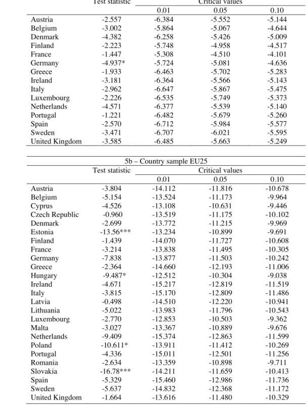
Moreover, according to the SURADF tests in Table 5, the general government

expenditure-to-GDP ratios seem to be non-stationary in most countries, but the null of a

unit root can be rejected at the ten per cent level of significance in one country

(Germany) for the EU15 panel, and in four countries (Estonia, Hungary, Poland and

Table 5 – SURADF stationarity tests with critical values for general government expenditure-to-GDP ratios

5a – Country sample EU15

Critical values

Test statistic

0.01 0.05 0.10

Austria -2.557 -6.384 -5.552 -5.144

Belgium -3.002 -5.864 -5.067 -4.644

Denmark -4.382 -6.258 -5.426 -5.009

Finland -2.223 -5.748 -4.958 -4.517

France -1.447 -5.308 -4.510 -4.101

Germany -4.937* -5.724 -5.081 -4.636

Greece -1.933 -6.463 -5.702 -5.283

Ireland -3.181 -6.364 -5.566 -5.143

Italy -2.962 -6.647 -5.867 -5.475

Luxembourg -2.226 -6.535 -5.749 -5.373 Netherlands -4.571 -6.377 -5.539 -5.140

Portugal -1.221 -6.482 -5.679 -5.260

Spain -2.570 -6.712 -5.984 -5.577

Sweden -3.471 -6.707 -6.021 -5.595

United Kingdom -3.585 -6.485 -5.663 -5.249 5b – Country sample EU25

Critical values

Test statistic

0.01 0.05 0.10 Austria -3.804 -14.112 -11.816 -10.678 Belgium -5.154 -13.524 -11.173 -9.964

Cyprus -4.526 -13.108 -10.631 -9.446

Czech Republic -0.960 -13.519 -11.175 -10.102

Denmark -2.699 -13.772 -11.215 -9.969 Estonia -13.56*** -13.234 -10.899 -9.691

Finland -1.439 -14.070 -11.727 -10.608

France -3.214 -13.838 -11.495 -10.305

Germany -7.838 -13.877 -11.503 -10.242 Greece -2.364 -14.660 -12.193 -11.006

Hungary -9.487* -12.512 -10.304 -9.038

Ireland -4.671 -15.217 -12.819 -11.519

Italy -3.815 -15.170 -12.809 -11.486

Latvia -0.498 -14.510 -12.220 -10.941

Lithuania -5.022 -13.983 -11.796 -10.543 Luxembourg -2.770 -12.853 -10.503 -9.362

Malta -3.027 -13.367 -10.889 -9.676

Netherlands -9.409 -15.374 -12.863 -11.599 Poland -10.611* -13.911 -11.412 -10.269

Portugal -4.336 -15.011 -12.501 -11.256 Romania -2.634 -13.359 -10.898 -9.711 Slovakia -16.78*** -14.211 -11.659 -10.413

Spain -5.329 -15.460 -12.986 -11.736

Sweden -5.637 -14.832 -12.368 -11.172

5c – Country sample EU26

Critical values

Test statistic

0.01 0.05 0.10 Austria -2.663 -14.757 -12.421 -11.096 Belgium -2.786 -13.495 -11.079 -9.907

Cyprus -0.320 -14.257 -11.609 -10.434

Czech Republic -3.154 -14.798 -12.174 -10.774 Denmark -3.010 -14.850 -12.050 -10.794 Estonia -11.258** -12.564 -10.234 -8.858

Finland -1.987 -13.049 -10.274 -9.090

France -2.845 -14.693 -12.065 -10.769

Germany -6.096 -14.673 -12.185 -10.873 Greece -2.285 -14.837 -12.394 -11.093

Hungary -9.661* -13.416 -10.914 -9.605

Ireland -2.512 -14.654 -11.951 -10.697

Italy -2.899 -16.217 -13.523 -12.257

Latvia -3.314 -15.135 -12.780 -11.587

Lithuania -1.811 -16.022 -13.533 -12.318 Luxembourg -2.989 -15.666 -13.006 -11.668

Malta -0.869 -14.243 -11.698 -10.456

Netherlands -3.842 -16.587 -14.116 -12.728 Poland -9.195* -12.564 -10.234 -8.858

Portugal -2.875 -16.414 -13.817 -12.467

Romania -7.018 -12.311 -9.736 -8.531

Slovakia -11.523* -15.260 -12.629 -11.245

Slovenia -3.458 -12.913 -10.250 -8.973

Spain -3.504 -16.930 -14.076 -12.773

Sweden -4.569 -16.415 -13.924 -12.586

United Kingdom -2.855 -8.952 -6.901 -6.034 * The SURADF column refers to the estimated Augmented Dickey–Fuller statistics obtained through the SUR estimation associated to the three EU15, EU25 and EU26 ADF regressions. Each of the estimated equation excludes a time trend. The three right-hand side columns contain the estimated critical values tailored by the simulation experiments based on 10,000 replications, following the work by Breuer et al. (2002). The symbols *, **, and *** denote statistical significant at the 10%, 5% and 1% level respectively.

Note: E25 excludes Bulgaria and Slovenia; E26 excludes Bulgaria.

To investigate the robustness of these results, particularly for the EU25 and EU26 panel

sets over the 1998-2006 and 2000-2006 periods, we carry out the recently developed

bootstrap tests of Smith et al. (2004), which use a sieve sampling scheme to account for

both the time series and cross-sectional dependencies of the data.5 The tests that we

consider are denoted t, LM , max, and min . All four tests are constructed with a unit

root under the null hypothesis and heterogeneous autoregressive roots under the

stationarity for at least one country.6 For the general government revenue-to-GDP

ratios, the results reported in Table 6 suggest that the unit root null cannot be rejected at

any conventional significance level for any of the four tests7 for the three EU15, EU25

and EU26 panel sets (the last two panels excluding now Poland) over respectively the

1960-2006, 1998-2006 and 2000-2006 periods and hence provide confirmatory

evidence of non-stationarity SURDAF results. For the general government

expenditure-to-GDP ratios, the results of the recently developed bootstrap tests of Smith et al.

(2004), reported in Table 6, confirm these findings for the three panel sets, EU15

excluding now Germany (since it passed the stationarity test in Table 5), EU25 and

EU26 excluding Estonia, Hungary, Poland and Slovakia, over the 1960-2006,

1998-2006 and 2000-1998-2006 periods respectively.

These findings permit to shed some light on the sometimes ambiguous results

previously obtained in Tables 2 and 3 with the Breitung, IPS, and Hadri panel unit root

tests. This is not surprising as the previous panel unit root tests rely on a joint test of the

null hypothesis while the SURADF tests each member country individually using a

system approach. Besides, Breuer et al. (2002, 2006) have shown that the SURADF has

double to triple the power of the ADF test in rejecting a false null hypothesis.

6

The t test can be regarded as a bootstrap version of the well-known panel unit root test of Im et al. (2003). The other tests are basically modifications of this test.

7

Table 6 – Results of Smith et al. (2004) panel unit root test for general government revenue and expenditure-to-GDP ratios

General government revenue General expenditure revenue Test Statistic Bootstrap

P-value*

Statistic Bootstrap P-value* EU15** (1960-2006)

t -1.742 0.227 -1.774 0.221

LM 3.762 0.281 3.413 0.346

max 0.518 0.997 -0.153 0.990

min 0.849 0.982 0.593 0.990

EU25*** (1998-2006)

t -1.191 0.732 -1.568 0.257

LM 4.091 0.129 3.612 0.242

max -0.608 0.513 -1.334 0.102

min -1.244 0.456 -2.223 0.124

EU26*** (2000-2006)

t -1.827 0.230 -1.074 0.785

LM 3.428 0.103 3.539 0.125

max -0.537 0.754 1.019 0.995

min 1.951 0.432 2.180 0.265

Note: rejection of the null hypothesis indicates stationarity at least in one country. *All tests are based on an intercept and 5000 bootstrap replications to compute the p-values. ** EU15 excluding Germany for general government expenditure-to-GDP ratios. *** EU25 and EU26 excluding Poland for general government revenue-to-GDP ratios, and excluding Estonia, Hungary, Poland and Slovakia for general government expenditure-to-GDP ratios.

It appears that we are in the case of three mixed panels, because some of the members

are stationary while others are not and the SURADF test clearly enables us to identify

for which members the general government revenue or/and expenditure taken as a

percentage of GDP are mean reverting and for which they are not. This information

obtained for each country in a panel framework taking into account the

contemporaneous cross-correlation information obtained from the SUR estimates is

crucial for assessing fiscal sustainability in each country of the three EU15, EU25 and

EU26 panel sets. As mentioned before, this encompassing analysis has not been pursued

4.3. Step 2: panel cointegration

Our investigations now proceed with the two following steps. Firstly, given the results

of the SURADF tests we define three new panel sets: EU14 which includes all countries

of the EU15 panel except Germany; EU21 and EU22 which correspond to the EU25

and EU26 previous panel sets without Estonia, Hungary, Poland and Slovakia. Indeed,

in these countries, at least one of the two series of general government revenue and

expenditure is integrated of order zero, hence preventing from carrying out

cointegration techniques. We then perform panel data cointegration tests of the second

generation (that allows for cross-sectional dependence among countries) between

government expenditure and revenue in the new defined EU14, EU21 and EU22 panel

sets.

Secondly, if a cointegrating relationship exists for all countries in at least one of the

EU14, EU21 and EU22 panel sets, we estimate the system

it i i it it

R D E G u , i=1,…,N; t=1,…,T (8)

by the Zellner (1962) approach to handle cross-sectional dependence among countries

using the SUR estimator. This way of proceeding enables us to estimate the individual

coefficients ȕi in a panel framework and hence to investigate fiscal sustainability for

each country taken individually. We finally test for homogeneity of ȕi across country

We now proceed by testing for the existence of cointegration between government

expenditures and revenues, taken as a percentage of GDP, using the very recent

bootstrap panel cointegration test proposed by Westerlund and Edgerton (2007). Unlike

the panel data cointegration tests of Pedroni (1999, 2004), generalized by Banerjee and

Carrion-i-Silvestre (2006), this test has the advantage that the joint null hypothesis is

cointegration. Therefore, in case of null non-rejection we know for sure that a

cointegration relationship exists for the whole set of countries of the panel set, which is

crucial here to assess fiscal sustainability. On the contrary, when performing the

Banerjee and Carrion-i-Silvestre (2006) methodology the problem arises that a single

series from the panel might be responsible for rejecting the joint null of non-stationary

or non-cointegration, hence not necessarily implying that a cointegration relationship

holds for the whole set of countries. This could be less helpful when investigating fiscal

sustainability since no information is provided on which panel member(s) is responsible

for this rejection, that is for which fiscal sustainability does not hold.

The new test developed by Westerlund and Edgerton (2007) relies on the popular

Lagrange multiplier test of McCoskey and Kao (1998), and permits correlation to be

accommodated both within and between the individual cross-sectional units. In

addition, this bootstrap test is based on the sieve-sampling scheme, and has the

appealing advantage of significantly reducing the distortions of the asymptotic test.8

The results, reported in Table 7 for a model including either a constant term or a linear

trend clearly indicate the absence of a cointegrating relationship between government

of 0.00 the null hypothesis of cointegration is always rejected, in line with the results of

Afonso and Rault (2007a) for a shorter panel sample.

Table 7 – Panel cointegration test results between government revenueand expenditure (Westerlund and Edgerton, 2007) a

EU14 (1960-2006)

LM-stat Asymptotic p-value

Bootstrap p-value Model with a constant term 7.864 0.000 0.165 Model including a time trend 8.285 0.000 0.001 EU21 (1998-2006)

Model with a constant term 0.703 0.241 0.631 Model including a time trend 3.998 0.000 0.576 EU22 (2000-2006)

Model with a constant term 1.057 0.145 0.504 Model including a time trend 4.930 0.000 0.677

Note: the bootstrap is based on 2000 replications.

a - The null hypothesis of the tests is cointegration between government revenueand expenditure.

Note: E14 excludes Germany; E21 excludes Bulgaria, Estonia, Hungary, Poland, Slovakia, and Slovenia; E26 excludes Bulgaria; E22 excludes Bulgaria, Estonia, Hungary, Poland, and Slovakia.

An opposite and more encouraging result is, however, obtained for a model including a

constant if one refers to the bootstrap critical values, indicating that for a significant

level smaller than 16.5 per cent, the null hypothesis is now not rejected for the period

1960-2006. Hence at the conventional 5 and 10 per cent levels of significance, we can

conclude that a cointegration relationship exists between government revenue and

expenditure ratios for the EU14 panel data set. This result now differs from those

reported in Afonso and Rault (2007a), who found that the hypothesis of fiscal policy

sustainability was rejected for the EU15 on the period 1970-2006, and indicates that a

longer time series sample may be important to assess fiscal sustainability.

Likewise, for the EU21 and EU22 panel sets, strong evidence is found in favour of the

refers to bootstrap critical values. This result is robust to the inclusion of a trend in

addition to the constant in the estimated regression. Such a result, however, does not

hold for a model including a constant and a trend if one relies on the asymptotic

p-values. Interestingly, and since the two last panel sets start essentially at the end of the

1990s, this evidence regarding the existence of a long-run relationship between

government revenue and expenditure is rather in line with the results from Afonso and

Rault (2007a) for the EU15, for the sub-period 1992-2006 (even if for a smaller set of

countries).

We then investigate whether public finances were sustainable for the model including a

constant term, using a Wald statistic to test whether the panel cointegration coefficient

of the general government expenditure-to-GDP ratios is equal to one or not in the

cointegrating regression where revenue is the dependent variable. Over the 1960-2006

periods and for the EU14 panel data-set the calculated Wald test statistic is 6.049 with

an associated p-value of 1.43%, which provides evidence in favour of the null of a

common unit slope equal to one, but only at the one percent level of significance.

Stronger evidence of the sustainability of public finances is obtained for the EU21 and

EU22 panel data set over the 1998-2006 and 2000-2006 periods since the calculated

Wald test statistics for the above hypothesis are respectively of 0.422781 and 0.005623,

the associated p-values being respectively of 51.55 and 94.02%.

4.4. Step 3: SUR cointegration relationships

We now estimate the system (8) for the EU14, EU21 and EU22 panel sets to assess the

approach, which is useful to address cross-sectional dependency. Those SUR estimation

results are reported in Tables 8a, b and c.

Table 8a – SUR estimation for the EU14 panel (1960-2006)

Country Coefficients

DE in eq. (8)

t-Statistic

Probability Country Coefficients

DE in eq. (8)

t-Statistic

Probability

Austria D 9.274 11.9 0.000 Italy D 6.692 4.8 0.000

E 0.770 47.5 0.000 E 0.694 22.3 0.000 Belgium D 9.410 7.2 0.000 Luxembourg D 3.942 3.3 0.001

E 0.706 27.4 0.000 E 0.936 28.3 0.000 Denmark D 6.836 5.3 0.000 Netherlands D 4.949 6.1 0.000

E 0.865 33.5 0.000 E 0.849 51.6 0.000 Finland D 9.553 8.1 0.000 Portugal D 6.145 9.0 0.000

E 0.833 32.1 0.000 E 0.712 38.0 0.000 France D 7.798 13.3 0.000 Spain D 5.264 9.8 0.000

E 0.791 63.3 0.000 E 0.781 52.1 0.000 Greece D 8.188 10.5 0.000 Sweden D 23.792 16.3 0.000

E 0.643 35.6 0.000 E 0.575 22.0 0.000 Ireland D 8.164 5.0 0.000 UK D 13.298 5.9 0.000

E 0.677 16.9 0.000 E 0.620 11.3 0.000 Note: Seemingly Unrelated Regression, linear estimation after one-step weighting matrix. Balanced system, total observations: 658.

Table 8b – SUR estimation for the EU21 panel (maximum time span, 1960-2006)

Country Coefficients

DE in eq. (8)

t-Statistic

Probability Country Coefficients

DE in eq. (8)

t-Statistic

Probability

Austria D 9.260 12.0 0.000 Latvia D 12.149 2.9 0.000

E 0.770 48.0 0.000 E 0.657 5.6 0.000 Belgium D 9.423 7.4 0.000 Lithuania D 20.856 12.8 0.000

E 0.705 28.3 0.000 E 0.362 8.4 0.000 Cyprus D -3.815 -0.8 0.369 Luxembourg D 3.747 3.3 0.001

E 1.004 9.7 0.000 E 0.941 30.5 0.000 Czech Republic D 32.744 13.3 0.000 Malta D -11.073 -1.1 0.242

E 0.155 2.9 0.000 E 1.105 5.2 0.000 Denmark D 6.893 5.4 0.000 Netherlands D 5.105 6.7 0.000

E 0.863 34.2 0.000 E 0.845 55.1 0.000 Finland D 9.453 8.1 0.000 Portugal D 6.103 9.0 0.000

E 0.834 32.8 0.000 E 0.713 38.7 0.000 France D 7.711 13.4 0.000 Romania D 13.027 3.9 0.000

E 0.792 64.9 0.000 E 0.611 7.5 0.000 Germany D 14.360 15.5 0.000 Spain D 5.273 10.1 0.000

E 0.639 30.9 0.000 E 0.780 53.8 0.000 Greece D 8.129 10.6 0.000 Sweden D 23.497 16.5 0.000

E 0.644 36.7 0.000 E 0.580 22.8 0.000 Ireland D 8.283 5.4 0.000 UK D 12.935 5.8 0.000

E 0.674 17.9 0.000 E 0.628 11.6 0.000

Italy D 6.499 4.7 0.000

E 0.698 23.0 0.000

Table 8c – SUR estimation for the EU22 panel (maximum time span, 1960-2006)

Country Coefficients

DE in eq. (8)

t-Statistic

Probability Country Coefficients

DE in eq. (8)

t-Statistic

Probability

Austria D 9.272 12.0 0.000 Latvia D 12.368 3.0 0.000

E 0.770 48.0 0.000 E 0.651 5.7 0.000 Belgium D 9.424 7.4 0.000 Lithuania D 20.872 12.8 0.000

E 0.705 28.4 0.000 E 0.362 8.4 0.000 Cyprus D -4.104 -0.9 0.331 Luxembourg D 3.715 3.3 0.001

E 1.011 9.8 0.000 E 0.942 30.6 0.000 Czech Republic D 32.669 13.4 0.000 Malta D -11.842 -1.2 0.206

E 0.156 2.9 0.000 E 1.121 5.3 0.000 Denmark D 6.909 5.4 0.000 Netherlands D 5.091 6.7 0.000

E 0.863 34.2 0.000 E 0.845 55.3 0.000 Finland D 9.449 8.1 0.000 Portugal D 6.107 9.0 0.000

E 0.835 32.8 0.000 E 0.713 38.7 0.000 France D 7.713 13.4 0.000 Romania D 13.379 4.2 0.000

E 0.792 64.9 0.000 E 0.602 7.8 0.000 Germany D 14.342 15.5 0.000 Slovenia D 0.000 2.1 0.030

E 0.639 31.0 0.000 E 1.000 8.0 0.000 Greece D 8.136 10.7 0.000 Spain D 5.280 10.2 0.000

E 0.644 36.7 0.000 E 0.780 53.9 0.000 Ireland D 8.286 5.4 0.000 Sweden D 23.478 16.5 0.000

E 0.674 17.9 0.000 E 0.580 22.9 0.000 Italy D 6.487 4.7 0.000 UK D 12.944 5.8 0.000

E 0.698 23.0 0.000 E 0.628 11.6 0.000 Note: Seemingly Unrelated Regression, linear estimation after one-step weighting matrix. Balanced system, total observations: 780.

According to our estimation results, although the coefficient E is always statistically

significant, and with the right sign, its magnitude is also below unity. Nevertheless, it

seems fair to point out that the size of the E coefficient is quite high in some cases and

above, for instance, 0.8, notably for Denmark, Finland, Luxembourg, and the

Netherlands.9 These results, which hold for all three country panels that we studied, can

be read as an indicator that public finances may have been relatively less unsustainable

in the past for the abovementioned four countries.

9

On the other hand, it is also possible to observe the lower magnitude of the estimated E

coefficient for several countries such as Belgium, Greece, Ireland, Italy, the UK or

Sweden, which reflects a bigger departure from a one-to-one linkage between

expenditures and revenues in the cointegration relationship. Interestingly, and as a result

of running significant budget deficits, those countries then experienced a divergent

behaviour of their respective debt-to-GDP ratio during continued phases in the period

1960-2006, which would theoretically increase in infinite horizon if the magnitude of E

were to remain too far away and below unity. Indeed, the expenditure ratios were

systematically above, and growing faster in some cases, than the revenue ratios for most

of the period in the cases of Belgium, Greece, Ireland, Italy and the UK while in

Sweden that difference was particularly acute in the first half of the 1990s.

Regarding the new EU Members States present in the third step of our analysis, the

estimated cointegration relationship shows a rather low magnitude of the E coefficient

for the cases of the Czech Republic and Lithuania, which can be driven by some spikes

that occurred in the expenditure ratios in the period under analysis.

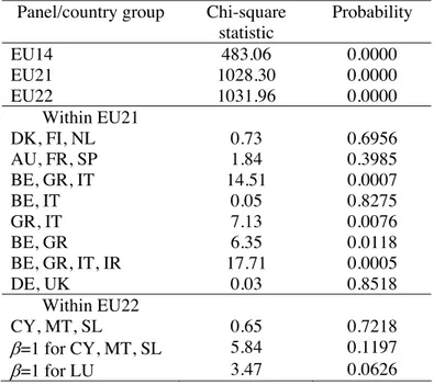
Finally, we also tested the homogeneity of ȕ across countries using a Wald test, which

may in principle be useful to uncover any common behaviour for some country

sub-groups. For instance, one could consider that it is more likely to pair countries with less

sustainable past public finances, and on the other hand lump together countries with

Table 9 – Testing the homogeneity of ȕ across countries

Panel/country group Chi-square statistic

Probability

EU14 483.06 0.0000

EU21 1028.30 0.0000

EU22 1031.96 0.0000

Within EU21

DK, FI, NL 0.73 0.6956

AU, FR, SP 1.84 0.3985

BE, GR, IT 14.51 0.0007

BE, IT 0.05 0.8275

GR, IT 7.13 0.0076

BE, GR 6.35 0.0118

BE, GR, IT, IR 17.71 0.0005

DE, UK 0.03 0.8518

Within EU22

CY, MT, SL 0.65 0.7218

E=1 for CY, MT, SL 5.84 0.1197

E=1 for LU 3.47 0.0626

Note: the null is that E is the same for all countries in the sub-group.

While the homogeneity hypothesis was always rejected for the overall three EU panel

sets, interestingly it held for some specific country pairings and sub-groups. For

instance, it is possible to see that the null of homogeneity for E, that is the similarity in

the responses of government revenues to changes in government expenditures, was not

rejected jointly for Denmark, Finland and the Netherlands, and also for the cases of

Austria, France and Spain. Additionally, a similar past behaviour of public finances was

also not rejected for the case of Belgium and Italy, which are two countries that

accumulated significant stocks of government debt during most of the period under

analysis. Finally, it is notable that the null of homogeneity (as well as of a unit

coefficient) in the cointegration relationship is not rejected for the cases of Cyprus,

Malta and Slovenia. Interestingly these are the first three countries, of the new EU

5. Conclusion

Even if there is no single fiscal policy in the EU, panel analysis of the sustainability of

public finances is certainly relevant in the context of 27 EU countries seeking to pursue

sound fiscal policies within the framework of the Stability and Growth Pact. Indeed, the

shared constraints on EU member countries’ fiscal policy under the SGP calls for a

panel approach alongside a country by country assessment. In this paper, starting from

the intertemporal government budget constraint, and taking advantage of non-stationary

panel data econometric techniques we assess the sustainability of public finances

covering several sub-periods within the period 1960-2006 and also defining different

country groupings for the 27 members of the EU.

We used a 3-step analysis where we employed (i) SURADF panel integration analysis,

which seems to be the first empirical application in the context of the sustainability of

public finances; (ii) panel bootstrap to test the null hypothesis of cointegration between

expenditure and revenue ratios; (iii) SUR methods to assess the magnitude of the

estimated coefficient of revenues in the cointegration relationship. This approach takes

advantage of the increased power of panel techniques and also provides specific

information regarding how far from fiscal sustainability a given country has been in the

past.

According to the results of several panel unit root tests, notably with the SURADF test,

general government revenue and expenditure-to-GDP ratios are not stationary for the

overwhelming majority of the EU27 countries. Additionally, at the conventional 5 and

relationship between government revenue and expenditure ratios for the EU14 panel

data set over the period 1960-2006. A similar conclusion regarding the existence of a

cointegration relation can be drawn for the country panel sets that include the more

recent members of the EU: EU21, for the period 1998-2006; and EU22, for the period

2000-2006.

Moreover, for the countries were a cointegration relation exists, we used the SUR

estimator, allowing for cross-country dependence among countries, to estimate the

coefficient of the expenditure ratio in a system were the revenue ratio is the independent

variable. However, and even if a cointegration vector was identified for all countries,

the estimated coefficient for expenditures, in the cointegration equations is usually less

than one. In other words, for the period 1960-2006, government expenditures in the

EU14 (in the EU21 and EU22 countries for the more recent sub-periods) exhibited a

higher growth rate than public revenues, questioning the hypothesis of fiscal policy

sustainability. These results suggest that fiscal policy may not have been sustainable for

most countries while it may have been less unsustainable for such countries as

References

Afonso, A. (2005). “Fiscal Sustainability: The Unpleasant European Case”,

FinanzArchiv, 61 (1), 19-44.

Afonso, A. and Rault, C. (2007a). “What do we really know about fiscal sustainability

in the EU? A panel data diagnostic”, European Central Bank Working Paper n° 820.

Afonso, A. and Rault, C. (2007b). “Should we care for structural breaks when assessing

fiscal sustainability?” Economics Bulletin, 3 (63), 1-9.

Ahmed, S. and Rogers, J. (1995). “Government budget deficits and trade deficits. Are

present value constraints satisfied in long-term data?” Journal of Monetary

Economics, 36 (2), 351-374.

Bai, J., Ng, S. (2004), "A PANIC Attack on Unit Roots and Cointegration",

Econometrica, 72 (4), 127-1177.

Banerjee, A. and Carrion-i-Silvestre, J. (2006). “Cointegration in Panel Data with

Breaks and Cross-section Dependence”, European Central Bank, Working Paper

591, February.

Breuer, J., McNown, R. and Wallace, M. (2002). “Series-specific unit root tests with

panel data”. Oxford Bulletin of Economics and Statistics 64, 527–546.

Breuer, J., McNown, R. and Wallace, M. (2006). “Misleading Inferences from Panel

Unit Root Tests: A Reply”, Review of International Economics, Vol. 14, No. 3, pp.

512-516, August 2006.

Campbell, J. Y., and P. Perron. (1991). ‘‘Pitfalls and Opportunities: What

Macroeconomists should Know about Unit Roots.’’ In O. Blanchard and S. Fishers

(eds.), NBER Macroeconomics Annual. Cambridge, MA: MIT Press.

Choi, I. (2006). “Combination Unit Root Tests for Cross-sectionally Correlated Panels”,

in Corbae, D., Durlauf, S. and Hansen, B. (eds), Econometric Theory and Practice:

Frontiers of Analysis and Applied Research, Essays in Honor of Peter C. B. Phillips,

Cambridge: Cambridge University Press.

Hadri, K. (2000). "Testing for Stationarity in Heterogeneous Panel Data", Econometrics

Journal, 3 (2), 148-161.

Hakkio, G. and Rush, M. (1991). “Is the budget deficit "too large?"” Economic Inquiry,

29 (3), 429-445.

Haug, A. (1991). “Cointegration and Government Borrowing Constraints: Evidence for

Im, K. and Lee, J. (2001). “Panel LM Unit Root Test with Level Shifts”, Discussion

paper, Department of Economics, University of Central Florida.

Im, K., Pesaran, M. and Shin, Y. (2003). “Testing for Unit Roots in Heterogeneous

Panels”,Journal of Econometrics, 115 (1), 53-74.

Levin, A., Lin, C.-F. and Chu, C.-S. (2002). “Unit Root Tests in Panel Data:

Asymptotic and Finite Sample Properties”, Journal of Econometrics, 108 (1), 1-24.

Maddala, G. and Wu, S. (1999). “A Comparative Study of Unit Root Tests and a New

Simple Test”, Oxford Bulletin of Economics and Statistics, 61 (1), 631-652.

McCoskey, S. and Kao, C. (1998). “A Residual-Based Test of the Null of Cointegration

in Panel Data”, Econometric Reviews, 17 (1), 57-84.

Moon, H. and Perron, B. (2004). “Testing for a Unit Root in Panels with Dynamic

Factors”,Journal of Econometrics, 122 (1), 8-126.

Pedroni, P. (1999). “Critical Values for Cointegrating Tests in Heterogeneous Panels

with Multiple Regressors”, Oxford Bulletin of Economics and Statistics, 61 (1),

653-670.

Pedroni, P. (2001). “Purchasing Power Parity Tests in Cointegrated Panels,” Review of

Economics and Statistics, 83, 727-31.

Pedroni, P. (2004). “Panel Cointegration; Asymptotic and Finite Sample Properties of

Pooled Time Series Tests with an Application to the Purchasing Power Parity

Hypothesis”,Econometric Theory, 20 (3), 597-625.

Pesaran, M. (2007). “A Simple Panel Unit Root Test in the Presence of Cross Section

Dependence”,Journal of Applied Econometrics, 22 (2), 265-312.

Prohl, S. and Schneider, F. (2006). “Sustainability of Public Debt and Budget Deficit:

Panel Cointegration Analysis for the European Union Member Countries”,

Department of Economics, Johannes Kepler University Linz, Working Paper No

0610.

Quintos, C. (1995). “Sustainability of the Deficit Process with Structural Shifts,”

Journal of Business & Economic Statistics, 13 (4), 409-417.

Smith, V., Leybourne, S. and Kim, T.-H. (2004). “More Powerful Panel Unit Root Tests

with an Application to the Mean Reversion in Real Exchange Rates.’’ Journal of

Applied Econometrics 19, 147–170.

Taylor, A. and Taylor, M. (2004). “The Purchasing Power Parity Debate”, Journal of

Taylor, M. and Sarno, L. (1998). “The Behavior of Real Exchange Rates During the

Post-Bretton Woods Period”, Journal of International Economics, 46 (2), 281-312.

Westerlund, J. and Prohl, S. (2006). “Panel Cointegration Tests of the Sustainability

Hypothesis in Rich OECD Countries”, forthcoming in Applied Economics.

Westerlund, J. and Edgerton, D. (2007). “A Panel Bootstrap Cointegration Test”,

Economics Letters, 97, pp. 185-190, 2007.

Westerlund, J. (2007). “Estimating Cointegrated Panels with Common Factors and the

Forward Rate Unbiasedness Hypothesis”. Journal of Financial Econometrics 5, pp.

491-522, 2007.

Zellner, A. (1962). "An efficient method of estimating seemingly unrelated regressions

and tests of aggregation bias”. Journal of the American Statistical Association, 57,