The responses of child labor, school enrollment, and grade repetition to the loss of parental earnings in Brazil, 1982-1999

Texto

(1)The Responses of Child Labor, School Enrollment, and Grade Repetition to the Loss of Parental Earnings in Brazil, 1982-1999. Marcelo Neri Centro de Políticas Sociais /IBRE, REDE e EPGE Fundação Getulio Vargas. Emily Gustafsson-Wright Guilherme Sedlacek Peter F. Orazem. Em Breve (2009) em livro a ser publicado na Palgrave Macmillan, organizado por: Peter F. Orazem, Zafiris Tzannatos and Guilherme Sedlacek. Título da publicação: Child Labor and Education in Latin America: An Economic Perspective.. 1.

(2) The Responses of Child Labor, School Enrollment, and Grade Repetition to the Loss of Parental Earnings in Brazil, 1982-1999. Marcelo Neri Centro de Políticas Sociais /IBRE, REDE e EPGE Fundação Getulio Vargas. Emily Gustafsson-Wright Guilherme Sedlacek Peter F. Orazem. Results in chapter 2 suggest that in Latin America, poverty and child labor are positively linked at least in some countries, and that poverty and educational attainment are more consistently negatively linked across all countries.1 Most of the research that has documented these links has concentrated on the impact of persistent poverty on child labor and time in school. Less understood is whether transitory shocks to household income also affect decisions regarding child time allocations. If poor households can absorb income shocks by borrowing against future income, then short-term income loss from unemployment, illness, or injury to adults in the household should not affect the schooling or work decisions of the children in the home. However, if poor households face constraints on borrowing because they lack collateral or other means of demonstrating ability to repay, then child work time may be used to substitute for lost adult work time. Even temporary exits from school can lead to permanent loss of human capital if school success is predicated on continuous participation. Jacoby and Skoufias (1997, 1998) link incompleteness in financial markets to lower human capital accumulation in a study examining the response of children's school attendance to seasonal fluctuations in the income of agrarian households in rural India. They find that children's time is used as a buffer or a form of self-insurance for unforeseen income losses. Flug et al. (1998) found that areas without financial markets had lower secondary enrollment 1. For other studies, see Grootaert and Patrinos (1999), Jensen and Nielsen (1997), Psacharopoulos (1997), and Tzannotos (1998), who found that low parental income leads to greater child labor. Paes de Barros and Lam. 2.

(3) rates.. Duryea (1998). found that in Brazil, when the father in a household becomes. unemployed, his children are 4% less likely to advance in grade. Parker and Skoufias (2002) found that increased unemployment rates significantly increased the probability of child drop-out. Beegle et al. (2002) and Edmonds (2002) find consistent results for Tanzania and South Africa, respectively. This study examines how the loss of earnings by the head of a household in Brazil affects how his children spend their time in school and work. The study opens with a simple theoretical explanation of how income shocks may lead to socially inefficient school drop-out and labor market entry by children in credit-constrained households. The theory is used to motivate an analysis of one-year transition rates from school to work and from school to no school. An analysis of nonpromotion rates also is motivated by the theory. The empirical model allows the impact of the earnings shock to differ by household income status before the earnings loss occurred. Children's time allocation in higher-income households was largely unaffected by the loss of earnings by the head. However, children in the poorest households were more likely to drop out, enter the labor force, and repeat the same grade in school. Because children who lag behind age-appropriate grade level are more likely to drop out or enter the labor market in the future, even those children whose education plans are not immediately altered may be permanently affected by the adverse consequences of the income shock on their chance for grade promotion. These results are consistent with the presumption that the poorest households are credit- constrained, so children in those households will be more vulnerable to short-term fluctuations in household income due to parental job loss. Consequently, social insurance that provides a safety net against adverse income shocks to the poorest households may help to prevent premature and socially inefficient labor market entry or school drop-out by children in the poorest households.. Theory The possible impact of household income shocks on child time in school or at work can be illustrated with a simple three-period variant of the Ben-Porath (1967) model. In the first stage, the child attends school full time, so attendance, A, = 1. In stage 2, 0 < A < 1, meaning the child divides time between school and work. In the third stage, the child specializes in working, setting A = 0. (1996), Gomes-Neto and Hanushek (1994), Lam and Schoeni (1993), and Mello, Souza, and Silva (1996) have found positive relationships between various measures of schooling outcomes and parents' income levels.. 3.

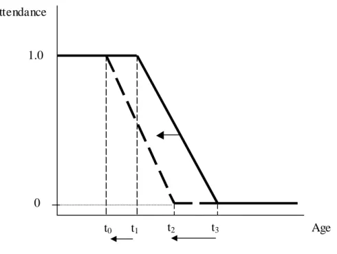
(4) To show how the length of stage 1 or stage 2 varies with shocks for income, it is assumed that there are positive but diminishing returns to school attendance so the amount of additional marketable skill developed per year of schooling decreases as years of schooling increase. Total marketable skill at any point in time is given by the wage the child can claim, W(Ht). Between any two periods, t = 0 and t= 1, the decision of whether to attend school will reflect the relative returns to schooling versus working. Let r = the interest rate. If the child attends school so A > 0, he will earn (1 - A) W(H0 ) in the current period and his value of time will be W(H1) = W(H(H0, A)), where human capital production depends positively on past human capital accumulation and attendance. If the child does not attend school, A = 0 and the child's value of time in both periods is W(H0). The child will attend school if (1 − A)W(H 0 ) +. W(H 0 ) W(H1 ) > W(H 0 ) + 1+ r 1+ r. or − AW(H 0 ) +. W(H1 ) − W(H 0 ) >0 1+ r. (1). Condition (1) says the child should attend if the present value of the wage increase attributable to schooling exceeds the cost of child time in school. If condition (1) holds with inequality, A will be set equal to 1 and the child will spend the period in stage 1. If the condition holds with equality, optimal attendance will be in stage 2, where 0 < A < 1. If the condition is violated, then the child will be in stage 3, where A = 0. Because returns to human capital are positive but diminishing as the level of human capital increases, the first term on the left-hand side of (1) grows progressively larger in magnitude and the second term on the left-hand side becomes progressively smaller as the child ages. Consequently, the child's schooling pattern will go from full-time to part-time to leaving school, as illustrated in figure 1. Income shocks will alter condition (1) for two reasons. First, income may make schooling more productive so that W(H1) – W(H0) rises with income. Second, the interest rate is a decreasing function of income if the poor are credit-constrained. As a consequence, the second term on the left-hand side of (1) decreases if the household suffers an adverse income shock, as illustrated in figure 2. A negative income shock shifts the attendance schedule to the left, causing children aged t0 to t1, who would otherwise attend school full-time, to enter the labor market. The shock also would induce children aged t2 to t3, who would otherwise. 4.

(5) attend part-time, to drop out of school. A large enough income shock could cause children in stage 1 to move all the way to stage 3.. Data and Empirical Strategies The data for this study are taken from the Pesquisa Mensal de Emprego (PME), a monthly employment survey conducted by the Brazilian census bureau. The survey concentrates on the six metropolitan areas of Brazil: Belo Horizonte, Porto Alegre, Recife, Rio de Janeiro, Salvador, and São Paulo. It elicits information from randomly selected households once a month for four consecutive months, drops them out of the sample for the next eight months, then interviews them again for four final months. The samples include about 5,000 households per city per month. The PME. is beneficial for this study because it tracks employment and income. characteristics of parents and their children aged 10 or older, allowing us to follow an individual child's enrollment, educational progress, and labor supply behavior over sixteen months. It also allows us to measure the relationship between decisions regarding child time use and the parents' employment and earnings history. This study uses data from February 1982 through February 1999. The sample is restricted to households with two parents and at least one child between 10 and 15 years of age. In the case of multiple children in that age range, the concentration is on the oldest child. The data set is further restricted to those households that completed all eight interviews. The concentration on two-parent households is to ensure that there are members of the household other than the child who could potentially alter labor supply behavior to smooth the household's income stream, were the head to lose labor earnings. To the extent that singleparent households would be even more vulnerable to income shocks because of the lack of other potential adult workers, the results understate the use of child labor as an incomesmoothing mechanism.. a. Endogenous Variables This study uses three transition indicators. Conditional on a child being in stage 1 at the end of the fourth month, the first indicator evaluates whether or not the child has dropped out of school twelve months later. In effect, this represents a transition from stage 1 to stage 3. The second measure, also conditional on stage 1 status in the fourth month, indicates whether the child has started working twelve months later. This represents a transition from stage 1 to either stage 2 or stage 3. The final measure is conditional upon status in stage 2, meaning that the child is both in school and working in the fourth month. The indicator is 5.

(6) whether or not the child has been promoted to the next grade. In figure 2, an adverse income shock could induce the child to attend less while still enrolled. Although the PME does not include an attendance measure, an increased probability of failure to advance to the next grade should correspond to a decline in intensity of investment in school.. b. Empirical Strategies The theory suggests that unforeseen income shocks will increase the probability that a child will move out of schooling and into child labor. This suggests conditioning a sample of children on status in schooling-stage 1 or schooling-stage 2 and then examining how an income shock to the household affects the transition probability into another stage. Formally, let S1t indicate that a child's schooling stage is 1 in period t, meaning that the child is in school and does not work; U Ht +1 is a dummy variable that takes the value of 1 if the household head loses his job in period t + 1. The child's schooling stage at a later date is observed and denoted Si,t+2, where I = 1, 2, 3. Guided by condition (1), the probability that a child leaves stage 1 is given by C W A P(Si ≠1, t + 2 /S1t ) = F(α + β U U Ht +1 + γ CW W C (H t ) + γ dW C dW (H t ) + γ A Wt + δZ t ) (2) W where F is the cumulative logistic distribution, α, β U , γ CW , γ dW C , γ A and δ are estimable. parameters, W C (H t ) is an indicator of the market value of child time, given human capital accumulated to time t, WtA is a vector of indicators of the market value of adult time,. dW C (H t ) is the expected change in wage from another year of schooling, and Zt is a vector of time and region dummy variables. The prediction from the theory is that an income shock to the household will hasten the child's exit from stage 1 so that β U > 0 . Factors that raise the market opportunities for the child would also hasten the exit from school so that γ CW > 0 , while factors that increase returns to schooling would slow exits. Increases in adult income would lower the probability of exiting stage 1, because the productivity of child time in school is enhanced and/or the parents face a lower discount rate on future earnings. The ability of the household to self-insure against income shocks should be related to the household's income status before the shock occurred. This suggests that the impact of an income shock would be the most severe in the poorest households. That hypothesis can be tested by interacting U Ht +1 with indicators of prior household income. Letting Yjt be a dummy variable indicating household income is in the jth quintile in the period before the shock, the. 6.

(7) 4. interaction terms. ∑ β UjYjt U Ht +1. are inserted into (2). If prior household income helps to. j=1. absorb income shocks, then β Uj should fall in magnitude as prior income quintile rises.. c. Market Opportunities For Children The child's opportunity cost of spending time in school will be the value of a child's time in production activities inside or outside the home. While some children work for pay, the vast majority of child laborers work for no pay. Consequently, the value of child time is approximated by inserting proxy measures for the elements of Ht. In particular, it is assumed that W C (H t ) =. 14. ∑. i =10. WiA AGE it + W M MALE. where AGEit is a series of dummy variables and will take the value of 1 if the child is age i and time t and zero otherwise, and MALE is a dummy variable indicating the child is a boy. The child's opportunity cost of schooling is expected to rise with age and boys are expected to claim a wage premium over girls. Children who are lagging behind in school face a slower increase in human capital per year in school, implying a smaller value of dW C (H t ) . d. Market Opportunities for Parents A parent may provide a potential source of substitute labor for an unemployed spouse, whether or not the parent currently works. Consequently, the relevant measure of adult income should reflect the human capital that the adults could supply to the market. For that reason, the adult earnings potential is represented by a sequence of dummy variables indicating education levels for the mother and father. A measure of the relative income status of the household also is included. There is a concern that household income measures are subject to measurement error and endogeneity with respect to labor supply choices (Deaton 1997). The measurement error problem is limited by using quintile income groupings, so modest errors will not move households into another quintile. In addition, the sample is restricted to households in which the head had positive labor earnings in the fourth month (for reasons that will become apparent) and the quintile placement is based solely on earnings of the head. Consequently, the potentially endogenous variation in labor supply behavior of the head is restricted. The sample is conditional on positive labor earnings by the head because of the need to define an income shock to the household. The strategy is to define the shock by the absence of labor earnings of the head in the last month observed. Consequently, at some time. 7.

(8) in the previous twelve months, the household head lost his source of labor earnings, and that situation persisted through the last period of observation.2 Note that this should give the household plenty of time to absorb the income shock , either by substituting other adult household member labor earnings to replace the lost earnings of the head, by sale of assets, or by other income-smoothing measures. Therefore, we may understate the adverse consequences of the income shock for child work or schooling if those responses have all occurred within the previous eight-month period when we do not observe how the child's time is allocated. On the other hand, if the adverse consequences of the income shock persist after this time, we can presume that the effects are not fleeting but will have a permanent effect on the child's employment and schooling patterns. The remaining measures control for systematic variation in labor demand across time and labor markets. A series of seasonal, municipal, and year dummy variables represent demand shifts that are common across workers. These dummies control for shifts in household income that are predictable due to known seasonal, local, or trend factors.. Results Table 1 presents sample statistics for various indicators of the use of child time for all children aged 10 to 15. In these urban areas, 6.7% of the children were not in school. The proportion out of school is modestly larger for boys than girls; however, boys are more than twice as likely to be in the labor force than girls. The majority of the boys who enter the labor market remain in school, but their academic progress may suffer. Boys are more likely than girls to lag behind grade level. Nevertheless, the proportions lagging behind are very high for both boys and girls at 65% and 55%, respectively. Table 2 presents transition rates for children over the sample period. Although boys and girls are equally likely to leave school at 0.5% per year, boys are more than twice as likely to start working and to start working while staying in school. It is interesting that the transition into stage 3 out of school is only slightly less likely from stage 1 than stage 2.. a. Transition Out of School Table 3 presents estimates of transition probabilities from stage 1 to stage 3. The model is estimated using a logistic model. The coefficients and associated t-statistics are reported, but the odds ratios are the most directly interpretable magnitudes.. 2. Duryea, Lam, and Levison (2001) defined the shock in terms of reported unemployment rather than zero labor earnings. They find similar but smaller responses to the shock measure.. 8.

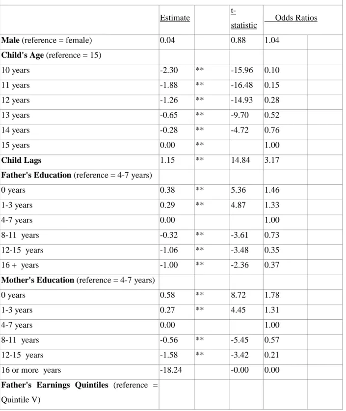
(9) Boys are 4% more likely to drop out than girls, but the difference is not significant. As the child ages, the probability of drop-out rises monotonically. A 15-year-old is ten times more likely to leave school than a 10-year-old. Children who lag behind their expected grade for age are three times more likely to leave school than are children who make normal progress. For both mothers and fathers, increasing parental education lowers the probability of exit. Children of fathers who never attended school are four times more likely to drop out than are children of college-educated fathers. The differences in school exit probability are even more sensitive to mothers' education levels. As the level of the household head's earnings prior to the shock rises, the probability that the child leaves school falls. Relative to households in the upper earnings quartile, children in the lowest quintile are 2.1 times more likely to drop out. The adverse earnings shock adds to the negative effect of low income on child dropout. The average effect across income quintiles implies that households in which the head loses earnings potential, even for a short time, are 24% more likely to have children leave school relative to households with similar incomes but a stable earnings stream. The joint test of significance of the five terms including UH easily rejects the null hypothesis of no effect. The negative effect of adverse income shocks on child schooling appears to be related to credit constraints. As prior income level rises, the adverse effect of the income shock decreases. The reported odds ratios are relative to the added adverse effect of the income shock on households in the top income quintile. Income shocks in the top quintile have virtually no effect on child schooling. In contrast, an income shock for households in the lowest income quintile has a 46% larger effect on the probability of child drop-out. It is more interesting to convert the estimates so that the odds ratios are relative to households in the same income group that did not experience an income shock. Those estimates are reported in the last column of table 3. The results are revealing. In the lowest income quintile, an adverse earnings shock raises the probability of drop-out by 43%. At the next three higher income quintiles, the adverse shock also increases the probability of drop out, but by smaller proportions.. b. Labor Market Entry Table 4 replicates the exercise for the probability that the child enters the labor market. This represents a move from stage 1 to stage 2 or stage 3. The results are similar to those in table 3: probability of labor market entry is 63% higher for boys than girls, rises with child age monotonically, and is higher for children who are lagging behind. More educated 9.

(10) parents are less likely to have their children work, and the probability of child labor market entry also drops monotonically as earnings quintile rises. All of these results are similar to the effects of these factors on school dropouts. The joint test of the significance of the interaction terms between the income shock and prior household income quintile indicated no significant effect. However, there is support for the presumption that income shocks matter at the lower end of the income distribution where individual coefficients were statistically significant. Loss of earnings of the head increase the odds of a child entering the labor market by 33% to 65% in the lowest of three earnings quintiles relative to households in the top earnings quintile that experienced a loss of earnings from the head. Compared to other households at the same income quintile, a household in the lowest quintile experiencing an adverse earnings shock is 23% more likely to have its children enter the labor market.. c. Nonpromotion Table 5 concentrates on children who are already in stage 2, in which they work while attending school. Nonpromotion is taken as an indication of relatively little investment of time in school. Results suggest that boys are more likely to fail, as are children who already lag behind in school. There is no apparent relationship between nonpromotion and child age, parental education, or household income. The joint test of the null hypothesis that the income shock had equal effects across income quintiles was strongly rejected. Children in the lowest income quintile had significantly greater probability of nonpromotion when their household experienced income loss of the head. At higher income quintiles, the adverse effect of the income shock on promotion disappears. Conclusions and Policy Considerations This study confirms a strong positive correlation between household income status and the probabilities of labor market entry and school drop-out. The finding suggests that income support programs can improve schooling outcomes for poor children. However, the study goes further to examine whether adverse shocks to a father's earnings causes a further increase in these probabilities. The answer depends on the poverty status of the household. Wealthier households appear able to self-insure against temporary income shocks caused by unemployment of the head. In those households, there is no evidence of changes in child time use in response to changes in parental labor market status. In the poorest households, however, loss of earnings by the household head increases the probability of drop-out and labor market entry, and also increases the likelihood of nonpromotion. This is consistent with. 10.

(11) the presumption that the poorest households may be credit-constrained and will use child labor to smooth adverse income shocks. There is some evidence that the adverse consequences of transitory income shocks have permanent adverse consequences for child schooling. The probability of drop-out and labor market entry increases once a child begins to lag behind in school. Consequently, to the extent that loss of earnings of the head leads to nonpromotion among children in the poorest households, there is a longer-term increased probability that the child will exit school at a young age and start working. To the extent that child labor and school drop-out are viewed as mechanisms by which poverty is transmitted across generations, these findings suggest that poor households may need some form of safety net to help them weather adverse income shocks in other ways than sending their children to work. Unemployment insurance schemes are already in place in Brazil, but they do not cover individuals who are displaced from informal activities, a large share of the workers in Brazil. The drop-out rate and labor market entry rate were highest for boys and older children, i.e., those with the highest market opportunities outside school. It is likely that the problem of child labor cannot be combated by policies that target the poor for income support without also addressing labor market opportunities for children. This could be done by tying access to minimum income maintenance programs to school attendance, measures of school progress, or verifiable reductions in child labor. Whether by raising perceived returns to time in school or by lowering perceived returns from early labor market entry, such programs would slow the transition out of school and into work.. 11.

(12) References Ben-Porath, Yoram. 1967. The Production of Human Capital and the Life Cycle of Earnings. Journal of Political Economy 75: 352-365.. Beegle, Kathleen, Rajeev H. Dehejia, and Roberta Gatti. Child Labor, Income Shocks and Access to Credit. World Bank Policy Research Working Paper no. 2652.. Deaton, Angus. 1997. The Analysis of Household Surveys: A Microeconometric Approach to Development Policy. Johns Hopkins University Press.. Duryea, Suzanne. 1998. Children's Advancement Through School in Brazil: The Role of Transitory Shocks to Household Income. Inter-American Development Bank. Mimeo.. Duryea, Suzanne, David Lam, and Deborah Levison. 2001. Effects of Economic Shocks on Children's Employment and Schooling in Brazil. Inter-American Development Bank. Mimeo.. Edmonds, Eric. 2002. Is Child Labor Inefficient? Evidence from Large Cash Transfers. Dartmouth.Mimeo. Flug, Karnit, Antonio Spilimbergo, and Erik Wachtenheim. 1998. Investment in Education: Do Economic Volatility and Credit Constraints Matter? Journal of Development Economics. 55: 465-481.. Fundação Instituto Brasileiro de Geografia e Estatística. 1983. Metodologia da Pesquisa Mensal de Emprego 1980. Rio de Janeiro, Brazil.. Fundação Instituto Brasileiro de Geografia e Estatística. 1991. Para Compreender a PME. Rio de Janeiro, Brazil.. Gomes-Neto, Joao Batista and Eric A. Hanushek. 1994. Causes and Consequences of Grade Repetition: Evidence from Brazil. Economic Development and Cultural Change 43: 117-148.. Grootaert, Christian and Harry Anthony Patrinos, eds. 1999. Policy Analysis of Child Labor: A Comparative Study. St. Martin's Press. Jacoby, Hanan G. and Emmanuel Skoufias. 1997. Risk, Financial Markets, and Human Capital in a Developing Country. Review of Economic Studies 64: 311-335.. 12.

(13) Jacoby, Hanan G. and Emmanuel Skoufias. 1998. Testing Theories of Consumption Behavior Using Information on Aggregate Shocks: Income Seasonality and Rainfall in Rural India. American Journal of Agricultural Economics 80(1): 1-14.. Jensen, P. and H. S. Nielsen. 1997. Child Labor or School Attendance: Evidence from Zambia. Journal of Population Economics 10(4): 407-424.. Lam, David and Robert Schoeni. 1993. Effects of Family Background on Earnings and Returns to Schooling: Evidence from Brazil. Journal of Political Economy 101: 710-740.. Mello e Souza, Alberto de and Nelson do Valle Silva. 1996. Income and Educational Inequality and Children's Schooling Attainment. Opportunity Foregone: Education in Brazil. Nancy Birdsall and Richard Sabot, eds. Inter-American Development Bank.. Parker, Susan W. and Emmanuel Skoufias. 2002. Labor Market Shocks and Their Impacts on Work and Schooling: Evidence from Urban Mexico. IFPRI. Mimeo.. Tzannotos, Zafiris. 1998. Child Labor and School Enrollment in Thailand in the 90's. Social Protection Discussion Paper No. 9818. World Bank.. 13.

(14) Figure 1: Stages of Investment in School Attendance. 1.0. 0 Age Stage 1. Stage 2. Stage 3. Figure 2: The Impact of Adverse Income Shocks on Investment in School. Attendance. 1.0. 0 t0. t1. t2. t3. 14. Age.

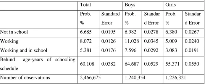
(15) Table 1: Static Indicators of School Performance and Child Labor (Children between 10 and 15 years of age) Total. Boys. Prob.. Standard Prob.. Standar. Prob.. Standar. %. Error. %. d Error. %. d Error. Not in school. 6.685. 0.0195. 6.982. 0.0278. 6.380. 0.0267. Working. 8.072. 0.0126. 11.028. 0.0345. 5.009. 0.0240. Working and in school. 5.381. 0.0176. 7.596. 0.0292. 3.083. 0.0191. 60.108. 0.0382. 64.687. 0.0529. 55.371. 0.0550. Behind. age-years of schooling. schedule Number of observations. 2,466,675. Girls. 1,240,354. 1,226,321. Source: Pesquisa Mensal de Emprego (PME) 1982/1999. Elaboration: CPS/FGV.. 15.

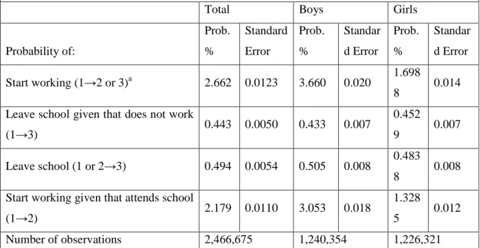
(16) Table 2: Dynamic Indicators of School Performance and Child Labor (Children between 10 and 15 years of age) Total. Boys. Prob.. Standard Prob.. Standar. Prob.. Standar. Probability of:. %. Error. %. d Error. %. d Error. Start working (1→2 or 3)a. 2.662. 0.0123. 3.660. 0.020. 0.443. 0.0050. 0.433. 0.007. 0.494. 0.0054. 0.505. 0.008. 2.179. 0.0110. 3.053. 0.018. Leave school given that does not work (1→3) Leave school (1 or 2→3) Start working given that attends school (1→2) Number of observations a. 2,466,675. Girls. 1,240,354. 1.698 8 0.452 9 0.483 8 1.328 5. 0.007. 0.008. 0.012. 1,226,321. Numbers in parentheses reflect transition from and to education stages.. 16. 0.014.

(17) Table 3: Logistic Estimation of the Probability a Child Leaves School Condition: In month 4, child is in stage 1 (attending school and not working) and head has positive earnings. t-. Estimate Male (reference = female). statistic. 0.04. Odds Ratios. 0.88. 1.04. Child's Age (reference = 15) 10 years. -2.30. **. -15.96. 0.10. 11 years. -1.88. **. -16.48. 0.15. 12 years. -1.26. **. -14.93. 0.28. 13 years. -0.65. **. -9.70. 0.52. 14 years. -0.28. **. -4.72. 0.76. 15 years. 0.00. **. Child Lags. 1.15. **. 14.84. 3.17. 0 years. 0.38. **. 5.36. 1.46. 1-3 years. 0.29. **. 4.87. 1.33. 4-7 years. 0.00. 8-11 years. -0.32. **. -3.61. 0.73. 12-15 years. -1.06. **. -3.48. 0.35. 16 + years. -1.00. **. -2.36. 0.37. 0 years. 0.58. **. 8.72. 1.78. 1-3 years. 0.27. **. 4.45. 1.31. 4-7 years. 0.00. 8-11 years. -0.56. **. -5.45. 0.57. 12-15 years. -1.58. **. -3.42. 0.21. 16 or more years. -18.24. -0.00. 0.00. 1.00. Father's Education (reference = 4-7 years). 1.00. Mother's Education (reference = 4-7 years). Father's Earnings Quintiles (reference = Quintile V). 17. 1.00.

(18) Quintile I. 0.75. **. 5.21. 2.11. Quintile II. 0.64. **. 6.41. 1.89. Quintile III. 0.57. **. 6.22. 1.77. Quintile IV. 0.31. **. 3.43. 1.37. Quintile V. 0.00. 1.00. Income Shocka UH (reference = Quintile V and UH = 0). -0.01. -0.05. 0.99. Quintiles I*UH. 0.38. 1.02. 1.46. [1.43]. Quintiles II*UH. 0.22. 0.69. 1.24. [1.22]. Quintiles III*UH. 0.27. 0.87. 1.31. [1.30]. Quintiles IV*UH. 0.17. 0.50. 1.19. [1.16]. Interactions (reference = QuintileV, UH=1)b. ___________________________________ Number of Observations: 56,080 Log Likelihood: -7290 Notes: * significance at the .10 level; ** significance at the .05 level. Regression also includes dummy variables for month, year, and metropolitan area. a. Joint test of UH and its interaction terms with quintile dummies is significant at the .05 level.. b. Odds ratios in brackets in the last column are relative to the same earnings quintile with UH=0.. 18.

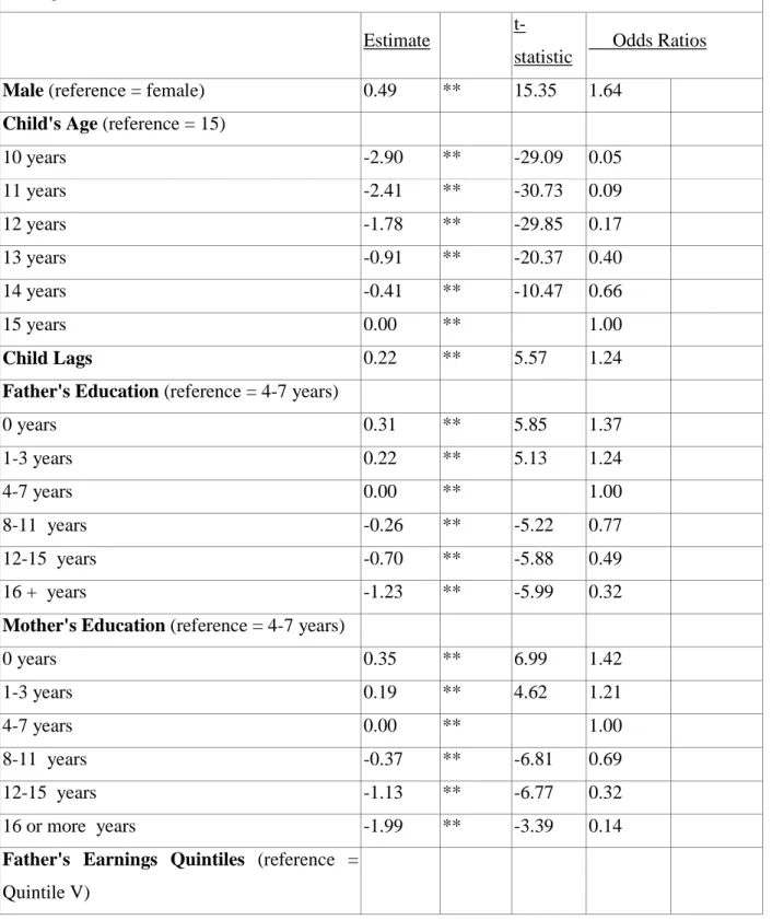
(19) Table 4: Logistic Estimation of the Probability a Child Enters the Labor Market Condition: In month 4, child is in stage 1 (attending school and not working) and head has positive earnings. t-. Estimate Male (reference = female). statistic. Odds Ratios. 0.49. **. 15.35. 1.64. 10 years. -2.90. **. -29.09. 0.05. 11 years. -2.41. **. -30.73. 0.09. 12 years. -1.78. **. -29.85. 0.17. 13 years. -0.91. **. -20.37. 0.40. 14 years. -0.41. **. -10.47. 0.66. 15 years. 0.00. **. Child Lags. 0.22. **. 5.57. 1.24. 0 years. 0.31. **. 5.85. 1.37. 1-3 years. 0.22. **. 5.13. 1.24. 4-7 years. 0.00. **. 8-11 years. -0.26. **. -5.22. 0.77. 12-15 years. -0.70. **. -5.88. 0.49. 16 + years. -1.23. **. -5.99. 0.32. 0 years. 0.35. **. 6.99. 1.42. 1-3 years. 0.19. **. 4.62. 1.21. 4-7 years. 0.00. **. 8-11 years. -0.37. **. -6.81. 0.69. 12-15 years. -1.13. **. -6.77. 0.32. 16 or more years. -1.99. **. -3.39. 0.14. Child's Age (reference = 15). 1.00. Father's Education (reference = 4-7 years). 1.00. Mother's Education (reference = 4-7 years). Father's Earnings Quintiles (reference = Quintile V). 19. 1.00.

(20) Quintile I. 0.49. **. 5.13. 1.63. Quintile II. 0.40. **. 6.51. 1.50. Quintile III. 0.38. **. 6.88. 1.47. Quintile IV. 0.24. **. 4.46. 1.27. Quintile V. 0.00. **. -0.29. *. -1.66. 0.75. Quintiles I*UH. 0.50. **. 2.02. 1.65. [1.23]. Quintiles II*UH. 0.28. 1.41. 1.33. [1.00]. Quintiles III*UH. 0.42. 2.06. 1.52. [1.14]. Quintiles IV*UH. 0.25. 1.15. 1.28. [0.96]. 1.00. Income Shocka UH (reference = Quintile V and UH = 0) Interactions (reference = QuintileV, UH=1)b. **. ___________________________________ Number of Observations: 56,080 Log Likelihood: -14087 Notes: * significance at the .10 level; ** significance at the .05 level. Regression also includes dummy variables for month, year, and metropolitan area. a. Joint test of UH and its interaction terms with quintile dummies is significant at the .05 level.. b. Odds ratios in brackets in the last column are relative to the same earnings quintile with UH=0.. Table 5: Logistic Estimation of the Probability a Child Fails to Advance to the Next Grade Condition: In month 4, child is in stage 2 (attending school and working) and head has positive earnings Estimat. t-statistic. e Male (reference = female). Odds Ratios. 0.30. **. 3.60. 1.35. 10 years. -0.56. *. -1.84. 0.57. 11 years. -0.13. -0.59. 0.88. 12 years. 0.23. 1.50. 1.25. 13 years. -0.07. -0.60. 0.93. Child's Age (reference = 15). 20.

(21) 14 years. -0.04. 15 years. 0.00. Child Lags. 0.39. -0.50. 0.96 1.00. **. 4.15. 1.47. Father's Education (reference = 4-7 years) 0 years. 0.11. 0.10. 1.12. 1-3 years. 0.13. 1.31. 1.13. 4-7 years. 0.00. 8-11 years. -0.08. -0.64. 0.93. 12-15 years. 0.27. 0.89. 1.31. 16 + years. 0.10. 0.22. 1.11. 0 years. 0.02. 0.21. 1.02. 1-3 years. 0.06. 0.65. 1.06. 4-7 years. 0.00. 8-11 years. -0.09. -0.69. 0.91. 12-15 years. -0.40. -0.10. 0.67. 16 or more years. -20.67. -0.00. 0.00. Quintile I. -0.01. -0.03. 0.99. Quintile II. 0.11. 0.76. 1.11. Quintile III. 0.23. 1.85. 1.26. Quintile IV. 0.04. 0.30. 1.04. 1.00. Mother's Education (reference = 4-7 years). 1.00. Father's Earnings Quintiles (reference = Quintile V). Quintile V Income Shock. *. 0.00. 1.00. a. UH (reference = Quintile V and UH = 0). -0.98. **. -2.15. 0.37. Quintiles I*UH. 1.24. **. 2.09. 3.47. [1.30]. Quintiles II*UH. 0.93. *. 1.80. 2.53. [.95]. Quintiles III*UH. 0.76. 1.49. 2.14. [.80]. Quintiles IV*UH. 0.74. 1.35. 2.09. [.78]. Interactions (reference = QuintileV, UH=1)b. 21.

(22) ___________________________________ Number of Observations: 3,557 Log Likelihood: -2253 Notes: * significance at the .10 level; ** significance at the .05 level. Regression also includes dummy variables for month, year, and metropolitan area. a. Joint test of UH and its interaction terms with quintile dummies is significant at the .05 level.. b. Odds ratios in brackets in the last column are relative to the same earnings quintile with UH=0.. 22.

(23)